


Abstract
During megathrust earthquakes, great ruptures are accompanied by large scale mass redistribution inside the solid Earth and by ocean mass redistribution due to bathymetry changes. These large scale mass displacements can be detected using the monthly gravity maps of the GRACE satellite mission. In recent years it has become increasingly common to use the long wavelength changes in the Earth's gravity field observed by GRACE to infer seismic source properties for large megathrust earthquakes. An important advantage of space gravimetry is that it is independent from the availability of land for its measurements. This is relevant for observation of megathrust earthquakes, which occur mostly offshore, such as the |$M_{\text{w}} \sim 9$| 2004 Sumatra–Andaman, 2010 Maule (Chile) and 2011 Tohoku-Oki (Japan) events. In Broerse et al., we examined the effect of the presence of an ocean above the rupture on long wavelength gravity changes and showed it to be of the first order.
Here we revisit the implementation of an ocean layer through the sea level equation and compare the results with approximated methods that have been used in the literature. One of the simplifications usually lies in the assumption of a globally uniform ocean layer. We show that especially in the case of the 2010 Maule earthquake, due to the closeness of the South American continent, the uniform ocean assumption is not valid and causes errors up to 57 per cent for modelled peak geoid height changes (expressed at a spherical harmonic truncation degree of 40). In addition, we show that when a large amount of slip occurs close to the trench, horizontal motions of the ocean floor play a mayor role in the ocean contribution to gravity changes. Using a slip model of the 2011 Tohoku-Oki earthquake that places the majority of slip close to the surface, the peak value in geoid height change increases by 50 per cent due to horizontal ocean floor motion. Furthermore, we test the influence of the maximum spherical harmonic degree at which the sea level equation is performed for sea level changes occurring along coastlines, which shows to be important for relative sea level changes occurring along the shore. Finally, we demonstrate that ocean floor loading, self-gravitation of water and conservation of water mass are of second order importance for coseismic gravity changes.
When GRACE observations are used to determine earthquake parameters such as seismic moment or source depth, the uniform ocean layer method introduces large biases, depending on the location of the rupture with respect to the continent. The same holds for interpreting shallow slip when horizontal motions are not properly accounted for in the ocean contribution. In both cases the depth at which slip occurs will be underestimated.
1 INTRODUCTION
During earthquakes seismic slip occurs on fault interfaces, but it also causes a movement of mass in the Earth's interior that leads to changes in the Earth's gravity field. With the launch of the Gravity Recovery and Climate Experiment (GRACE) satellite mission, large scale gravity changes can be globally observed on a monthly basis, providing a new tool to study fault slip of very large (|$M_{\text{w}} \sim$| 9) earthquakes. The GRACE mission consists of two satellites that follow the same orbit, but separated approximately 220 km along track, and can observe monthly gravity changes with a spatial resolution of about 400 km (Tapley et al.2004). Since the occurrence of the |$M_{\text{w}}$| 9.1 2004 Sumatra–Andaman earthquake, a number of studies extracted the coseismic gravity change from the GRACE data and compared it with model results (e.g. Han et al.2006; Ogawa & Heki 2007; de Linage et al.2009), usually based on seismological or land-based geodetic data. While smaller in magnitude, the |$M_{\text{w}}$| 8.8 Maule (Chile) earthquake produced sufficiently large mass displacements to be detected by GRACE, as demonstrated by Heki & Matsuo (2010) and Han et al. (2010). A year later, Matsuo & Heki (2011) and Zhou et al. (2012) showed that the 2011 |$M_{\text{w}}$| 9.0 Tohoku-Oki (Japan) earthquake was observable in the long wavelength gravity field as observed by GRACE. Han et al. (2011) demonstrated that these GRACE-observed gravity changes could be used to infer the properties of the earthquake source. Cambiotti & Sabadini (2013) used GRACE data to invert for the hypocentre and seismic moment tensor of the Tohoku-Oki earthquake.
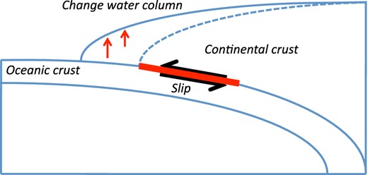
In the case of suboceanic earthquakes, changes in bathymetry have a first-order effect on coseismic gravity changes (de Linage et al.2009; Broerse et al.2011; Cambiotti et al.2011). Namely, when the bathymetry changes during an earthquake—up to a few metres of uplift and subsidence have been measured for recent megathrust earthquakes (Meltzner et al.2006; Farías et al.2010)—the height of the water column is adjusted, resulting in a redistribution of water. Uplift of the seafloor results in a local water mass removal and subsidence leads to a local water accumulation, see the scheme of Fig. 1. The total coseismic gravity change is thus a summation of solid Earth and ocean mass changes. These individual contributions should be understood in order to properly relate gravity changes to the properties of fault slip, such as its main depth, its orientation and magnitude. Main contributors to seismic gravity changes include:
Changes in topography: Uplift means a local increase in solid Earth mass, hence an increase in local strength of the gravity field. Similarly, uplift of an internal density contrast increases mass locally when the density of the lower layer is higher than that of the overriding layer.
Bathymetry changes: Since the ocean reacts to bathymetric uplift by forming an equipotential surface again, water mass is locally removed, implying a decrease of the gravity field.
Compressibility of the solid Earth: Solid Earth expansion expels mass from an expanding area, causing a local decrease in mass and thus gravity field, which is surrounded by a region of increased mass and gravity.
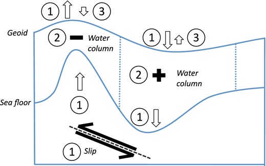
Schematic description of the coseismic effect of an ocean presence on gravity changes. (1) As the geoid surface represents the sea level at rest, coseismic changes in geoid height minus bathymetry changes represent the coseismic change in relative sea level. Uplift and subsidence of the seafloor due to thrust faulting are drawn, next to the related changes in the gravity field that are represented as geoid changes. (2) As the bathymetry change is two orders of magnitude larger than the geoid height change, around the uplifted region the water column will decrease and around the subsided region the water column will increase. (3) A smaller water column implies a local decrease in mass, resulting in a geoid height drop with respect to the increase of step 1 (left) and a larger water column at the subsided region leads to a secondary geoid height increase (right). Note: While changes in water column also change the loading of the ocean floor and thus trigger elastic deformation of the solid Earth, it shows that this type of deformation is very small with respect to the direct coseismic deformation (Broerse et al.2011). Hence we omit water load-induced deformation in this figure. Non-linear effects due to feedback between geoid changes, bathymetry changes and relative sea level are not depicted as well.
While most studies compare GRACE coseismic signals with model approaches that are based on slip distributions from external sources, recently it has become more common to invert for earthquake source parameters using GRACE-data only, such as after the very strong |$M_{\text{w}}$| 8.8 2010 Maule (Chile) (Wang et al.2012b; Han et al.2013) and the |$M_{\text{w}}$| 9.0 2011 Tohoku-Oki (Japan) earthquakes (Han et al.2011; Cambiotti & Sabadini 2012; Wang et al.2012a; Cambiotti & Sabadini 2013; Han et al.2013). With the exception of Cambiotti & Sabadini (2012), these studies used some approximations to the ocean contribution to coseismic gravity change. These often involve the assumption of a uniform ocean layer, no conservation of ocean mass, no self-gravitation of the ocean and the absence of feedback from elastic rebound due to water load changes. In Broerse et al. (2011) we applied a sea level equation for internal loading [similar to Melini et al. (2010)] for modelling the ocean contribution to coseismic gravity changes that can handle these aspects consistently. In this paper, we extend our previous study with an analysis of these approximations, which allows us to see how well other methods perform in modelling seismic geoid changes. Additionally, we examine the influence of the maximum spherical harmonic truncation degree to the modelled gravity when relative sea level peaks along the coast.
Furthermore, we introduce a novel approach to compute the ocean contribution to coseismic gravity changes that also takes into account horizontal motions of the ocean floor. Horizontal displacement of a steeply sloping ocean floor likely contributed to about half of the water column uplift after the 2011 Tohoku event as shown by Hooper et al. (2013). Horizontal displacements thus potentially contribute to gravity changes as well.
In studying the ocean response to coseismic gravity and bathymetry changes we address the following questions:
Is the assumption of a uniform ocean in the presence of continents around the ruptured area valid?
Can the sea level equation be performed at a low truncation degree in case only low degree gravity changes are needed?
What is the contribution of self-gravitation of water, elastic loading of the ocean floor and conservation of water mass?
When the ocean floor slopes significantly, to what extent does horizontal displacement contribute to gravity changes?
This paper is organized as follows: first we briefly reintroduce the sea level equation that we use for computing sea level changes due to earthquakes and its effect on gravity changes. This is followed by an analysis of the uniform ocean approximation, the effect of self-gravitation and elastic ocean floor loading and conservation of water mass. Furthermore we investigate the role of the maximum spherical harmonic degree for which the sea level equation is performed. Finally, we examine the contribution of horizontal displacements to gravity changes.
2 THE SEA LEVEL EQUATION FOR SEISMIC PERTURBATIONS REVISITED
To describe a sea level that incorporates both the self-attraction of water mass, and the elastic and viscoelastic response of the ocean floor due to water load changes, the sea level equation was developed by Farrell & Clark (1976). It has been widely used to model the changes in sea level due to the accretion and melt of large ice sheets during the glacial cycle, and the deformation of the solid Earth that was induced by these water and ice load changes; a process known as glacial isostatic adjustment (GIA). Recently, Melini et al. (2010) provided a version of the sea level equation for seismic perturbations and in Broerse et al. (2011) its use for coseismic gravity changes was discussed. Here we summarize the main characteristics of the sea level equation and its numerical application, for a complete discussion see Broerse et al. (2011).
3 THE COSEISMIC SEA LEVEL EQUATION DECONSTRUCTED
3.1 The uniform ocean assumption
Because the coseismic gravity changes studied in recent literature all concern subduction-zone earthquakes at continental margins,1 the possibility of the sea level equation to discriminate ocean and land areas is likely to make a difference with respect to a uniform ocean. Namely, part of the subsidence or geoid height decrease that comes with shallow subduction earthquakes may be over land areas, where no ocean mass change takes place. Of the three recent large subduction earthquakes, the 2004 Sumatra–Andaman, 2010 Maule and 2011 Tohoku-Oki earthquakes, the Maule earthquake was closely located to the vast land mass of the South American continent, whereas the Tohoku-Oki earthquake originated farther offshore. Consequently the largest subsidence was at sea offshore Japan, not at mainland Japan itself. The Sumatra–Andaman earthquake occurred below the Andaman sea, close to the Nicobar and Andaman islands, but the majority of the uplift and subsidence is again expected at the seafloor or around small islands. For that reason the largest influence of being able to distinguish between marine and terrestrial areas is expected for the 2010 Maule earthquake, for which reason we take this earthquake as a case study.
Solid Earth deformation and gravity potential changes have been computed by the analytical normal mode method (Vermeersen & Sabadini 1997; Sabadini & Vermeersen 2004) which treats the Earth as a radially stratified, compressible and self-gravitating spherical body. Earth properties are derived from PREM (Dziewonski & Anderson 1981), and are listed in Table S1. We make use of the ETOPO1 topography database (Amante & Eakins 2008) that we resampled from a 4 min grid to a 0.1° grid. Earthquake responses are modelled using a large number of seismic point sources (Piersanti et al.1995), where we obtain the description of the Maule earthquake slip geometry from Delouis et al. (2010). Furthermore we briefly review results for the 2004 Sumatra–Andaman and 2011 Tohoku-Oki events.
3.1.1 High spatial resolution results: lmax = 450
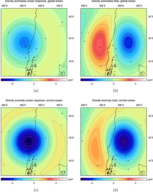
The inputs for the sea level equation are: vertical deformation R0 and geoid anomaly G0, both determined using the solid earth model (Fig. 2) and computed up to spherical harmonic degree lmax = 450. This truncation degree is the practical limit in resolution for our program as at higher degrees the code becomes numerically unstable, while lmax = 450 provides a sufficient spatial resolution for modelling gravity changes of megathrust earthquakes. Both responses have the typical dipole shape due to slip on a thrust fault, its peak values are given in Table 1. The contribution of the ocean to coseismic geoid heights is given in Fig. 3(a) and combined with the input geoid in Fig. 3(b). The ocean contribution for a uniform ocean has a dipole shape and lowers both peaks of the original geoid input (see Fig. 1). Switching to the realistic ocean, the first thing that is noticed is the disappearance of the positive pole in the ocean-only effect, as seen in Fig. 3(c). The ocean contribution consists of a single negative pole with a larger maximum than when a uniform ocean is assumed. This leads to total coseismic geoid height change that has a completely different asymmetry ratio compared to the uniform ocean case: 0.7:1 versus 1.4:1 (Table 1); that is the uniform ocean case overpredicts the positive part and underpredicts the negative signal (compare Figs 3b and d).
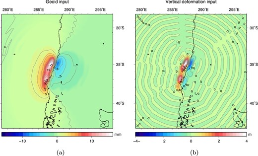
Input for the sea level equation: (a) initial coseismic geoid anomaly, (b) initial coseismic vertical deformation, both determined using the solid earth model.
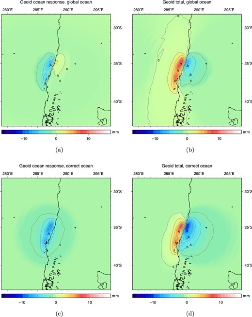
Geoid anomaly output of the sea level equation using a uniform ocean or the ocean function (eq. 1), which maps the relative sea level changes to the correct ocean areas: (a) Uniform ocean: additional geoid anomaly due to the ocean response. (b) Uniform ocean: total geoid anomaly including solid Earth and ocean contributions. (c) Realistic ocean: additional geoid anomaly due to the ocean response. (d) Realistic ocean: total geoid anomaly including solid Earth and ocean contributions.
Maximum negative values, maximum positive values and asymmetry ratio (maximum : minimum amplitudes) for the input geoid height, ocean contribution to geoid height and the sum of these two. Solutions are given for a realistic ocean, incorporating a detailed division between oceanic and continental areas, and a uniform ocean. Maximum geoid anomaly values in mm. Gravity anomalies at lmax = 40 are given in μGal and vertical deformation in metres.
| Realistic ocean | Uniform ocean | ||||||
|---|---|---|---|---|---|---|---|
| Min | Max | Asymmetry | Min | Max | Asymmetry | ||
| lmax = 450 | |||||||
| Vertical deformation | −2.4 | 3.9 | 1.6:1 | − 2.4 | 3.9 | 1.6:1 | |
| Input geoid anomaly | −8.5 | 15.7 | 1.9:1 | − 8.5 | 15.7 | 1.9:1 | |
| Ocean effect geoid anomaly | −8.0 | – | − 6.5 | 1.7 | |||
| Total geoid anomaly | −10.8 | 7.8 | 0.7:1 | − 6.8 | 9.3 | 1.4:1 | |
| lmax = 40 | |||||||
| Vertical deformation | − 0.02 | 0.11 | 5.4:1 | −0.02 | 0.11 | 5.4:1 | |
| Input geoid anomaly | −1.3 | 2.0 | 1.6:1 | − 1.3 | 2.0 | 1.6:1 | |
| Ocean effect geoid anomaly | −2.5 | 0.0 | − 4.2 | 0.8 | |||
| Total geoid anomaly | −2.2 | 0.1 | 0.1:1 | − 1.4 | 0.8 | 0.5:1 | |
| Ocean effect gravity anomaly | −7.5 | 1.2 | − 4.2 | 0.8 | |||
| Total gravity anomaly | −7.0 | 2.7 | 0.4:1 | − 5.0 | 4.0 | 0.8:1 | |
3.1.2 Low spatial resolution results: lmax = 40
The same results are presented for lmax = 40, which corresponds to the practical limit in resolution for which we can observe earthquake related gravity changes from GRACE data. Input geoid anomaly and vertical deformation at lmax = 40 are presented in Fig. 4. Results are determined up to and including degree 450 and afterwards truncated at degree 40, peak values are again given in Table 1. Here can be seen that geoid anomalies from the solid earth model at lmax = 40 result in a comparable asymmetry ratio w.r.t. results at lmax = 450, while the vertical deformation becomes predominantly positive at longer wavelengths. The uniform ocean case produces a mainly negative ocean contribution to the coseismic geoid heights (Fig. 5a). With respect to the initial geoid input, the resulting geoid anomaly (mainly the positive pole) is diminished in amplitude (Fig. 5b and Table 1). Using a realistic ocean, the ocean contribution is again mainly negative but with a larger amplitude than in the uniform ocean case (Fig. 5c). Therewith the ocean effect largely eliminates the positive peak and deepens the negative geoid anomaly (Fig. 5d). A comparable difference between a uniform ocean or realistic ocean is seen for the model results expressed as gravity anomalies (see Fig. A1).
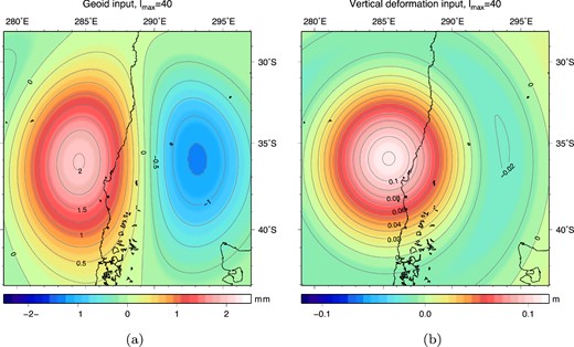
Input for the sea level equation, truncated at spherical harmonic degree 40: (a) initial coseismic geoid anomaly, (b) initial coseismic vertical deformation, both determined using the solid earth model.
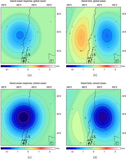
Geoid anomaly output of the sea level equation using the ocean function, which maps the relative sea level changes to the correct ocean areas, truncated at spherical harmonic degree 40: (a) Uniform ocean: additional geoid anomaly due to the ocean response. (b) Uniform ocean: total geoid anomaly including solid Earth and ocean contributions. (c) Realistic ocean: additional geoid anomaly due to the ocean response. (d) Realistic ocean: total geoid anomaly including solid Earth and ocean contributions.
3.1.3 Discussion
Using an ocean-land differentiation has a large influence on modelled coseismic geoid or gravity anomaly changes for seismic events occurring in the vicinity of coasts, at full resolution as well as using an lmax = 40, as exemplified by the 2010 Maule case. In this case the model predicts the magnitude of the positive poles to become 16 per cent smaller and the magnitude of the negative poles becomes 59 per cent larger with respect to the uniform ocean case at lmax = 450 (Table 1). As already visible in Fig. 2, in the case of the Maule earthquake the areas that undergo subsidence are located on land (due to the relative proximity of the trench to the coast). Consequently, differentiation between ocean and land will increase the effect of seafloor uplift on geoid heights. The same ocean test implemented at lmax = 40 produces equally considerable differences. With respect to the uniform ocean results, the magnitude of the negative pole becomes (in terms of geoid and gravity anomalies, respectively) 57/40 per cent larger for the negative pole and 80/33 per cent smaller for the positive pole when a realistic ocean is used. This implies that, in case of earthquakes that occurred just off the coast, modelling a realistic ocean is equally essential for coseismic gravity studies that make use of GRACE data, as well as for geoid studies where the full resolution is needed. The model error introduced by a uniform ocean is larger for geoid anomalies than for gravity anomalies as the former contains more long wavelengths signals. The need for a realistic ocean becomes increasingly important when lower truncation degrees are chosen or additional smoothing is applied as longer wavelength gravity signals are more prone to continent–ocean transitions.
An identical numerical experiment is performed for three forward models for the 2011 Tohoku-Oki earthquake (Hayes 2011; Wei et al.2011; Hooper et al.2013). Depending on the slip model chosen, the experiment revealed more modest geoid height changes due to an inclusion of a realistic ocean. At lmax = 40, 33 per cent to 4 per cent larger values for the negative pole geoid anomalies and 22 to 5 per cent larger values for the negative pole gravity anomalies were calculated with respect to the uniform ocean case. The largest changes are based on the Hayes (2011) model, the smallest on the model by Wei et al. (2011). However, as can be seen in the work by Zhou et al. (2012), the slip model of Wei et al. (2011) results in vertical deformation that better describes the GPS vertical displacements along the east coast than the Hayes (2011) model. A reason for the relatively small influence of a realistic ocean for the Tohoku-Oki modelling can be found in the fact that the predicted maximum subsidence is found offshore. For the 2004 Sumatra–Andaman earthquake a realistic ocean changes the modelled geoid heights with 2 and 8 per cent, respectively, for negative and positive poles at lmax = 40, with no qualitative changes in spatial pattern.
The general effect of omitting an ocean-land division is that for a given slip model, the modelled geoid height change becomes more positive. When a uniform ocean model is used for interpretation of gravity observations, one of the effects is that the slip will appear to be deeper than its actual depth, as deeper slip increases the ratio positive peak to negative peak (Cambiotti et al.2011; Han et al.2013).
3.2 Signal loss due to truncation at low degree spherical harmonics
When the sea level equation is solved following a pseudo-spectral approach, all calculations are performed in the spherical harmonic domain, except for the mapping of the global relative sea level change |$\Delta S\!\mathcal {L}$| on the oceans (eq. 3). This partial calculation in the spectral domain results in potentially different results when the sea level equation is solved up to a high degree (here lmax = 450) and results are subsequently truncated at a lower degree, say lmax = 40, or, when the sea level equation is conducted at a maximum degree of 40. This applies when vertical deformation peaks close to the coast line, such as in the case of the Maule earthquake, and to some minor extent for the Tohoku-Oki and Sumatra–Andaman earthquakes. Fig. 6 shows ΔS0 which is calculated as: (1) spherical harmonic expansion up to lmax = 40 (eq. 4), (2) mapping with the ocean function in the spatial domain (eq. 3) and (3) renewed spherical harmonic expansion up to lmax = 40 (needed for determination of the water column, eq. 6). It is clearly visible that, since a large part of the unmapped |$\Delta S\!\mathcal {L}$| covers continental area, the resulting ΔS0 in the spectral domain has lost a large part of the signal as peak values decrease by 17 per cent. The long wavelengths pertaining to lmax = 40 are simply unfit to properly represent the change in relative sea level after mapping on ocean areas. This results in a 37 per cent too low magnitude of the negative part and a seven times to high positive part of the total modelled geoid height change. Instead of an asymmetry ratio of 0.06:1 an incorrect ratio of 0.7:1 would be found. In terms of gravity anomalies the model gives a 29 per cent too low negative peak and 75 per cent too high positive peak by performing the sea level equation at lmax = 40 directly; asymmetry values incorrectly becomes 0.9:1 instead of 0.4:1.
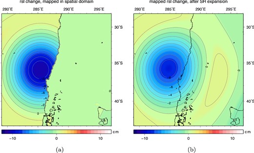
Relative sea level change, using a maximum spherical harmonic degree lmax = 40. (a) Initial relative sea level change ΔS0 after mapping on the ocean. (b) Same relative sea level change expanded in spherical harmonics with lmax = 40. Note the loss of signal after the spherical harmonic expansion, truncated at lmax = 40.
The same test has been applied for the Tohoku-Oki earthquake and Sumatra–Andaman earthquake where running the sea level equation at lmax = 40 leads to errors in coseismic geoid negative and positive peak values of −14(/+48) per cent [Wei et al. (2011) slip model], −28 per cent/+100 per cent [Hayes (2011) slip model], −24(/+42) per cent [Hooper et al. (2013) slip model] and 0 per cent/+12 per cent [Chlieh et al. (2007) Sumatra–Andaman slip model]. When a slip model results in a very small absolute amplitude of the positive pole the errors are given in between brackets. To analyse the maximum degree at which the sea level equation has to be run in order to obtain a converged geoid height change at lmax = 40, we show the maximum error for the Maule case in Fig. 7. For this case, the solution has converged when we solve the sea level equation at a degree of 350 or higher. Concluding, it is important to compute relative sea level changes at a high degree even when the application requires a lower one.
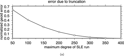
Errors in geoid height, truncated at lmax = 40, with increasing maximum degree for which the sea level equation is solved using the Maule case. Errors are determined by taking the maximum difference compared to the converged solution that solves the sea level equation up to degree 450. Errors are normalized using the absolute peak value of the converged solution. Errors for gravity anomalies are not displayed, but show a nearly identical behaviour.
3.3 Effects of loading, self-gravitation and conservation of ocean mass
Instead of iterating the sea level equation (eq. 2) until convergence of the relative sea level has been reached one can take the first order approximation ΔS0. This means that the sea level is no longer self-consistent as no deformation due to change in water load or self-gravitation of the ocean is taken into account and water mass is no longer conserved. This resembles the approach used by for example Han et al. (2006) (who used a half-space model that also neglects the Earth's sphericity), Heki & Matsuo (2010) and Matsuo & Heki (2011) (while these authors also neglect the ocean-land division). The authors include the ocean effect by using the difference in water and crustal densities for calculating the effect of topography change on gravity. Fig. 8 shows the difference between the converged solution for the coseismic geoid height and the initial geoid height when ΔS0 is used in eq. (6) and all love numbers are set to zero. It shows that the contribution of self-gravitation, conservation of water mass and elastic deformation has only a minor effect on the total geoid as the maximum magnitude is small relative to the total geoid anomaly: 0.15 mm versus –10.88 mm. The dominantly positive signal can be explained as coming from elastic rebound due to a local decrease in water mass. The asymmetry of the pattern arises from self-gravitation of water: due to a decrease in the water column, more water is removed locally. Consequently, peaks of the geoid dipole are changed by 1–2 per cent for converged results compared to first order approximation of geoid anomalies, and by 5 per cent at a truncation degree of 40. The maximum amplitude of the relative sea level changes less than 1 per cent in the subsequent iterations. Melini et al. (2010) report large contributions of subsequent iterations for the 2004 Sumatra–Andaman earthquake to the coseismic relative sea level change at a 20° distance, but do not describe effects on geoid anomalies. At locations far away from the rupture the influence of non-linearity and ocean mass conservation indeed becomes larger with respect to the zero-order approximation ΔS0. However, at these distances ΔS has already dropped to very low values. Possibly for some far-field tide-gauge locations the converged ΔS may become important in the long run, in case postseismic viscoelastic relaxation triggers long-wavelength uplift around the fault, as pointed out by Melini et al. (2010). Nonetheless, the sea level equation has limited added value for interpretation of coseismic relative sea level data.
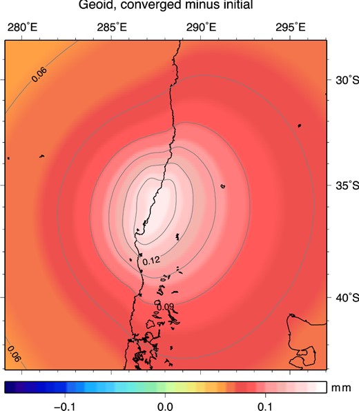
Converged coseismic geoid anomaly minus initial geoid anomaly for the 2010 Maule earthquake, indicating the contribution of self-gravitation of water, conservation of water mass and the deformation of the ocean floor due to changed surface loading. Maximum spherical harmonic degree is 450 and a realistic ocean is taken into account.
4 EFFECT OF HORIZONTAL DISPLACEMENT ON RELATIVE SEA LEVEL CHANGES
A dip angle of 5° up to 80 km from the trench after which the fault bends steeper at a dip angle of 15° for the remainder, as follows by the wide-angle seismic reflection study of Fujie et al. (2006).
Strike angle is 194.4°.
Slip patches measure 20 km downdip and are distributed at depths between 872 m and 51.3 km on a 450 km wide fault plane.
Schematic view of bathymetry changes due to horizontal movement towards a trench of a steep ocean floor. Dashed line represents the pre-earthquake continental crust position.
To study the sensitivity of the contribution of horizontal motions with slip depth we model for each separate depth gravity changes both with and without horizontal motion. At each depth we smoothly distribute slip over the 1-D profile, peaking halfway with 1 m dip slip, such that all depth segments represent the same integral of slip over the fault area. Fig. 10 shows the amplitudes of the positive and negative peaks in geoid and gravity anomalies at lmax = 40 with and without the effect of horizontal motion. The figure shows that especially the negative peak that is located over mainland Japan is very sensitive to horizontal motion for slip down to 25 km depth: for slip at depths between 900 m and 6 km the inclusion of sea level changes due to horizontal seafloor movement doubles the negative peak value (for geoid heights as well as gravity anomalies) and the effect of horizontal motion decreases with increasing depth. We notice that up to 24 km depth horizontal ocean floor motion contributes to the long wavelength (lmax = 40) coseismic geoid and gravity changes. The positive peak is affected by horizontal motions as well, but, as it's amplitude is small for shallow slip, differences will be harder to observe in noisy data. The decreasing effect of horizontal movement with increasing depth can be explained by two aspects: for increasing slip depth the peak horizontal movement decreases, and at the same time the location of peak surface displacement moves away from the trench (hence the area with largest bathymetry gradients).
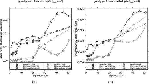
Contribution of horizontal ocean floor deformation to coseismic (a) geoid height changes and (b) gravity anomalies for slip patches with increasing depth. Slip patches follow the fault geometry of the Hooper et al. (2013) slip model and for every depth interval the same slip profile has been modelled. Figure shows model results including and excluding the contribution of horizontal deformation. Model results based on a uniform ocean and excluding horizontal motions are depicted as well. Black lines denote the amplitude of the negative peak, grey lines the amplitude of the positive peaks. Results have been truncated at lmax = 40.
Next to the 1-D fault test we investigate the importance of horizontal motion on coseismic gravity changes by applying the sea level equation to two different slip models of the Tohoku-Oki event. The first is the previously mentioned slip distribution of Hooper et al. (2013) that is based on an inversion of GPS data, seafloor pressure data and seafloor geodesy data combined with solid Earth deformation models as well as tsunami models. As in this model the slip reaches very shallow depths, the weighted average of the slip depth is 9.3 km. On the other hand, the USGS model by Hayes (2011) is based on teleseismic broadband waveforms and estimates a much deeper average slip depth of 20.3 km.
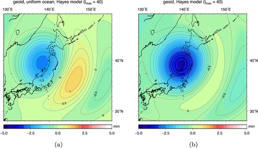
In Fig. 11 geoid height changes at lmax = 40 are given for both slip models, where the left panels do not take into account the effect of horizontal motion on bathymetry changes, while the right panels explicitly include this effect. Except for the different patterns of coseismic geoid height change between both slip models [the deeper slip of Hayes (2011) results in a more clear dipole pattern], for both slip models the inclusion of horizontal deformation results in a larger negative geoid height change and smaller positive peaks. The same results expressed in terms of gravity anomalies show a comparable decrease in gravity due to horizontal movement of the seafloor (see Fig. A2). When the effect of horizontal deformation is taken into account: the negative peak in coseismic geoid increases by 50 per cent (40 per cent for the gravity anomalies) based on the Hooper et al. (2013) slip model; the geoid negative peak value increases by 16 per cent (11 per cent for gravity anomalies) when using the Hayes (2011) slip model. In both cases the geoid height change has become entirely negative. The additional negative geoid height due to horizontal displacement can be understood from Fig. 12, that shows an extra increase in bathymetry caused by horizontal motions, such that water mass is driven away by the additional ocean floor uplift. On the other hand, the modelled radial deformation consists of both uplift and subsidence. Table 2 shows an overview of the peak values for both slip models. Here can be observed that when results are expressed as gravity anomalies, spatial patterns contain a positive part which decreases as well due to horizontal ocean floor motion. Positive peak values for results expressed in gravity anomalies decrease by 16 per cent and 37 per cent for the Hooper et al. (2013) and Hayes (2011) models. This implies that the ratio between positive and negative peak gravity anomaly decreases: for example for the Hayes (2011) slip model from 0.48:1 to 0.31:1.
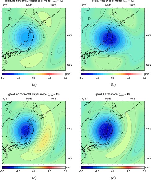
Coseismic geoid height changes predicted by the Hayes (2011) and Hooper et al. (2013) slip models, truncated at lmax = 40. Panels on the left show results without taking into account horizontal ocean floor displacement and subsequent bathymetry change. Panels on the right do include bathymetry changes resulting from horizontal displacement.
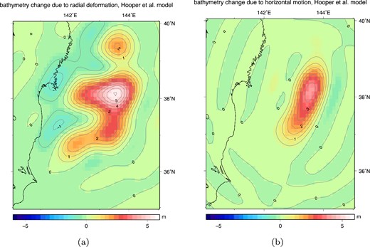
Modelled bathymetry changes at lmax = 450 according to the Hooper et al. (2013) slip model, due to: (a) radial deformation; (b) horizontal deformation.
Peak values for the modelled coseismic geoid height change and gravity anomalies for model runs with and without the effect of horizontal deformation on bathymetry. Asymmetry is defined as the ratio of positive peak to negative peak. For comparison we also list values for model runs that assumed a uniform ocean to see the accumulated effect of a realistic ocean and horizontal motions.
| Peak values | Hooper et al. slip model | Hayes et al. slip model | |||||
|---|---|---|---|---|---|---|---|
| Min | Max | Asymmetry | Min | Max | Asymmetry | ||
| Geoid height change (mm) |$l_{\text{max}}$| = 40 | |||||||
| No horizontal, uniform ocean | −2.3 | 0.3 | 0.13 : 1 | −2.7 | 1.2 | 0.44 : 1 | |
| No horizontal | −2.5 | 0.2 | 0.08 : 1 | −3.6 | 0.8 | 0.22 : 1 | |
| Including horizontal | −3.8 | 0.01 | 0.01 : 1 | −4.2 | 0.2 | 0.06 : 1 | |
| Gravity anomalies (μGal) lmax = 40 | |||||||
| No horizontal, uniform ocean | −7.7 | 2.8 | 0.36 : 1 | −10.2 | 6.3 | 0.61 : 1 | |
| No horizontal | −8.1 | 2.8 | 0.35 : 1 | −12.4 | 5.9 | 0.48 : 1 | |
| Including horizontal | −11.6 | 3.3 | 0.28 : 1 | −13.7 | 4.3 | 0.31 : 1 | |
The same test for inclusion of horizontal motion in determination of bathymetry changes has been performed for the 2004 Sumatra–Andaman and 2010 Maule earthquakes based on the Chlieh et al. (2007) and Delouis et al. (2010) slip models. Here we have found only minor changes by including the effect of horizontal deformation: at lmax = 40 modelled peak coseismic geoid height increases by only 2 and 6 per cent, respectively. The contribution of horizontal motion to the change in bathymetry will increase when the gradient of the bathymetry is larger or when the horizontal component of deformation becomes larger with respect to the vertical component. Especially the large horizontal displacements caused by the Tohoku-Oki earthquake—more than 50 m displacement has been observed (Ito et al.2011)—explain the large contribution of horizontal displacement to gravity, compared to the Sumatra–Andaman and Maule cases, for which we have modelled up to 10.1 and 5.8 m of horizontal displacement (at lmax = 450).
5 DISCUSSION
We analysed a number of modelling aspects of the ocean contribution to coseismic geoid height or gravity change. The two aspects that have the largest effects: a realistic ocean-land differentiation and horizontal motions of the ocean floor, both generate a more negative coseismic gravity pattern with respect to models excluding these aspects. In cases where both the ocean–land differentiation and horizontal motions have shown to be important, such as the Tohoku-Oki earthquake, even relatively modest contributions of the individual contributions will accumulate in a more significant impact. For example, for the Hayes (2011) slip model our forward model results in a 55 per cent larger negative peak in geoid height change with respect to the commonly used model that incorporates a uniform ocean and neglects horizontal effects (Fig. 13 and Table 2). In the Tohoku-Oki case, gravity change due to shallow slip is mostly affected by horizontal ocean floor motion and gravity change due to deep slip by a decrease in ocean contributions because of land presence, see Fig. 10. As can be seen here, coseismic gravity change patterns due to slip deeper than 25 km will become radically different when the differentiation between land and ocean is handled correctly: a model without ocean will provide positive peaks larger than negative peaks for slip below 30 km depth, while correct models will always produce dominantly negative patterns (at least for the Tohoku case). When GRACE derived gravity changes are interpreted using seismic point sources and horizontal motions and land presence are neglected, this will lead to biases in estimated properties as source depth, seismic moment or dip angle. Depending on the fault geometry we have to model 5–10 km deeper slip to obtain the same pattern of gravity change compared to the simplified models.
Comparison between models assuming (a) a uniform ocean and no contributions of horizontal motion and (b) the full model including a realistic ocean and contributions of horizontal motion. Here coseismic geoid height changes, truncated at lmax = 40, are based on the Hayes (2011) slip model.
6 CONCLUSIONS
The redistribution of ocean mass due to bathymetry changes has a first order effect on gravity changes, however there are two important aspects of modelling the bathymetry change that are not taken into account in the majority of studies that interpret coseismic gravity changes: (1) modelling a land-ocean differentiation for earthquakes occurring along the coast and (2) taking into account the contribution of horizontal displacement of sloped ocean floors for shallow earthquakes.
Modelling a realistic land–ocean division is essential for the interpretation of coseismic gravity changes due to earthquakes on faults close to the shore. At high spatial resolutions, as well as for a comparison with GRACE data, the inclusion of continental areas makes a large difference and radically changes the amplitudes and patterns of the coseismic geoid anomaly. Only when the earthquake occurs relatively far from the continent (e.g. the 2004 Sumatra–Andaman earthquake) the uniform ocean model simplification is acceptable. This is not the case for the 2010 Maule event, as, at lmax = 40, modelled peak coseismic geoid height increases by 57 per cent when a realistic land–ocean distribution is adopted (an increase by 40 per cent when expressed in terms of gravity anomalies). None of the recent studies about coseismic gravity changes induced by the Maule earthquake took into account the essential ocean-land differentiation (Han et al.2010; Heki & Matsuo 2010; Wang et al.2012b; Han et al.2013). For modelling gravity changes after the 2011 Tohoku-Oki event differentiation between land and ocean becomes important depending on how much slip is thought to be downdip, as deep slip will lead to more subsidence on mainland Japan. For the slip models under consideration, peak geoid height changes with respect to a uniform ocean model increases by 28–14 per cent. When a uniform ocean is assumed in inversion studies for fault zones close to large land masses, the GRACE derived co-seismic signal will be misinterpreted, resulting in biases for slip depth or seismic moment release estimates.
Secondly, when modelling or interpreting gravity changes due to shallow slip beneath a sloped ocean floor, bathymetry change due to horizontal displacement becomes of the same order of magnitude as bathymetry changes due to vertical deformation. We show that for shallow slip at small dip angles including horizontal motions can double coseismic negative peak geoid height or gravity changes, while this effect decreases for deeper slip. In our case, below 24 km the influence of horizontal motions becomes negligible for geoid height or gravity changes at the typical GRACE resolution (lmax = 40). Reviewing the effect of horizontal displacements for two distinct Tohoku-Oki slip models, we have shown that when slip is assumed to be concentrated close to the trench [on average at 9.3 km depth for the Hooper et al. (2013) slip model], the peak in coseismic geoid height change increases by 50 per cent. In the case slip is assumed to be located deeper [on average 20.3 km depth for the Hayes (2011) slip model], peaks in coseismic geoid height still increases by 16 per cent, and the cumulative increase is 55 per cent with respect to the uniform ocean case. In both Tohoku cases the coseismic geoid height pattern has become more dominantly negative.
Other processes correctly modelled by our approach, such as feedback from seafloor deformation and conservation of ocean mass represent only small signals in coseismic geoid height and change of relative sea level. Finally, we show that even if results of the sea level equation are needed for low spherical harmonic degrees only, the sea level equation should be solved at high degrees when large relative sea level changes are expected along coastlines. Due to the pseudospectral approach to solve the sea level equation, signal will leak from high to low spherical harmonic degrees, and affects any application that focuses on the effect of changes in relative sea level on the long wavelength gravity field.
The authors would like to thank the editor K. Heki and the reviewers K. Matsuo and G. Cambiotti for their review and suggestions. Taco Broerse acknowledges financial support from the SRON/NWO grant GO-AO/20 and ISES.
With the single exception of the 2012 Indian Ocean strike-slip earthquake (Han et al.2013).
REFERENCES
APPENDIX: RESULTS IN TERMS OF GRAVITY ANOMALIES
Gravity anomaly output of the sea level equation using the ocean function, which maps the relative sea level changes to the correct ocean areas, truncated at spherical harmonic degree 40: (a) Uniform ocean: additional gravity anomaly due to the ocean response. (b) Uniform ocean: total gravity anomaly including solid Earth and ocean contributions. (c) Realistic ocean: additional gravity anomaly due to the ocean response. (d) Realistic ocean: total gravity anomaly including solid Earth and ocean contributions.
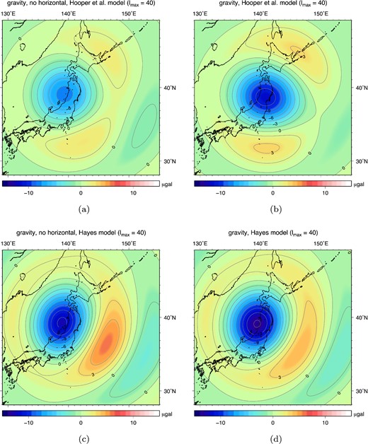
Coseismic gravity anomalies predicted by the Hayes (2011) and Hooper et al. (2013) slip models, truncated at lmax = 40. Panels on the left side show results without taking into account horizontal ocean floor displacement and subsequent bathymetry change. Panels on the right side do include bathymetry changes resulting from horizontal displacement.
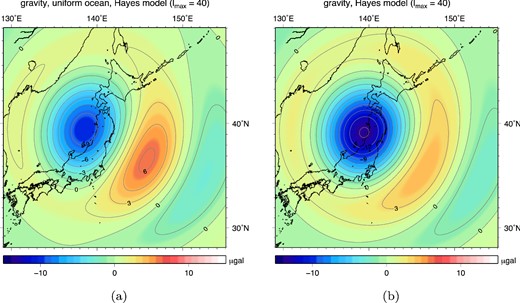
Comparison between models assuming (a) a uniform ocean and no contributions of horizontal motion and (b) the full model including a realistic ocean and contributions of horizontal motion. Here coseismic gravity anomalies, truncated at lmax = 40, are based on the Hayes (2011) slip model.
SUPPORTING INFORMATION
Additional Supporting Information may be found in the online version of this article:
Table S1. Parameters for the elastic earth model, volume averaged from PREM (Dziewonski & Anderson 1981) using the 200 s reference period and discarding the ocean layer. r is the distance with respect to the centre of the Earth, ρ is the density of the layer, μ is the rigidity and λ the first Lamé parameter. (http://gji.oxfordjournals.org/lookup/suppl/doi:10.1093/gji/ggu315/-/DC1 )
Please note: Oxford University Press is not responsible for the content or functionality of any supporting materials supplied by the authors. Any queries (other than missing material) should be directed to the corresponding author for the article.
