


Abstract
Passive seismic methods using earthquakes can be applied for extracting body waves and obtaining information of subsurface structure. In this study, we retrieve direct and reflected plane waves by applying seismic interferometry to the recorded ground motion from a cluster of regional earthquakes. We apply upgoing/downgoing P/S wavefield decomposition, time windowing, and multidimensional deconvolution to improve the quality of the extraction of reflected waves with seismic interferometry. The wavefield separation and seismic interferometry based on multidimensional deconvolution allow us to reconstruct PP, PS, SP and SS reflected waves without unwanted crosstalk between P and S waves. From earthquake data, we obtain PP, PS and SS reflected plane waves that reflect off the same reflector, and estimate P- and S-wave velocities.
1 INTRODUCTION
Body waves obtained from earthquakes (especially teleseismic events) have been used for imaging deep structure (crust–mantle, e.g. Bostock & Sacchi 1997; Bostock & Rondenay 1999; Baig et al.2005; Dasgupta & Nowack 2006). Receiver-function analysis is one technique to obtain information of subsurface structure by estimating traveltime differences between P and PS converted waves (e.g. Langston 1979; Li et al.2000; Assumpção et al.2002). Seismic interferometry (Aki 1957; Claerbout 1968; Wapenaar 2004) is also used for analyses of passive seismic waves including earthquake records. One can apply seismic interferometry to body waves generated by earthquakes and obtain images of subsurface structure (e.g. Abe et al.2007; Tonegawa et al.2009; Ruigrok et al.2010; Ruigrok & Wapenaar 2012). Abe et al. (2007) found that the image obtained from seismic interferometry has higher resolution than retrieved from receiver functions, but seismic interferometry creates spurious reflectors caused by higher-order multiples and crosstalk between P and S waves, which can be reduced by averaging over many earthquakes. Higher-resolution Green's functions are also obtained by estimating and deconvolving source functions from earthquake data recorded by a receiver array (Bostock 2004). The target for most body-wave seismic interferometry studies is deep structure, and comparably few studies aim at imaging the shallow crust (Ryberg 2011; Yang et al.2012; Behm & Shekar 2014). Seismic interferometry has been developed for analysing data trace by trace, and Wapenaar et al. (2008a,b) improve seismic interferometry by using multidimensional deconvolution (MDD). Although MDD interferometry requires one to separate wavefields depending on the direction of wave propagation and to solve an inverse problem, MDD overcomes several limitations (e.g. attenuation, complicated incident waves, and source distribution) of trace-by-trace interferometry (see Section 4.3).
In this study, we apply trace-by-trace and MDD seismic interferometry to earthquake data to retrieve direct and reflected plane waves. We first propose a technique of wavefield decomposition at the free surface. Using this decomposition, we separate observed two-component wavefields into upgoing/downgoing P/S wavefields, which is necessary for MDD interferometry. Next, we introduce earthquake data observed at the LaBarge field in Wyoming. Then we show a mathematical description of seismic interferometry and step-by-step improvement of interferometric wavefields by applying different techniques to the earthquake data.
2 UPGOING/DOWNGOING P/S WAVEFIELD DECOMPOSITION
A number of studies propose different techniques for wavefield separation: using, for example, dual sensors (Loewenthal & Robinson 2000), Helmholtz decomposition (Robertsson & Muyzert 1999; Robertsson & Curtis 2002), over/under towed-streamer acquisition (Moldoveanu et al.2007) and two steps of acoustic and elastic decomposition (Schalkwijk et al.2003). Dankbaar (1985) proposed a filter to separate upgoing P and SV waves from multicomponent seismic records. Wavefield separation improves wavefields obtained from interferometry to focus on target reflections (Mehta et al.2007; Vasconcelos et al.2008; van der Neut & Bakulin 2009). When receivers are embedded in a medium (e.g. ocean-bottom and borehole sensors), observed wavefields can be decomposed based on the direction of the wave propagation. Therefore, one can restrict the radiation pattern of virtual sources to suppress some spurious reflections caused by incomplete data acquisition for seismic interferometry (Mehta et al.2007). Because receivers are deployed at the free surface in our data, we cannot suppress the spurious multiples by separating wavefields based on the direction of wave propagation. We employ time windows to reduce the spurious multiples (Bakulin & Calvert 2006), and apply wavefield decomposition for separating the direction of wave propagation, which is necessary for MDD (Wapenaar et al.2011b) and for suppressing crosstalk of P and S waves.

Plane-wave reflection system and coordinates for the wavefield decomposition in Section 2. The horizontal grey line shows the free surface (indicated by |$\rightthreetimes \rightthreetimes$|), and the downward triangle on the line is a receiver. The black arrows near the receiver define the positive directions of observed records. The dashed lines illustrate portions of upgoing/downgoing P/S plane wave fronts. The black arrows near the dashed lines describe the positive directions of each vector wavefield. Solid black lines connected to dashed lines indicate the ray paths of each wavefield, and the triangles on the solid lines the direction of propagation. The angles θP and θS are the angles of incidence for P and S waves, respectively.
Notations of physical parameters and wavefields.
| Notation | Description | Relationship with other parameters |
|---|---|---|
| ω | Angular frequencya | |
| α | P-wave velocity at the layer below the free surface | |
| β | S-wave velocity at the layer below the free surface | |
| ρ | Density | |
| σij | Stress in the ij component | |
| μ | Lame's parameters | μ = β2ρ |
| λ | Lame's parameters | λ = (α2 − 2β2)ρ |
| θp | Angle of the P incident wave with respect to the free surface | |
| θs | Angle of the S incident wave with respect to the free surface | |
| k | Horizontal wavenumber | k = ω sin θp/α = ω sin θs/β |
| νp | Vertical wavenumber for P wave | |$\nu _p = \omega \cos \theta _p/\alpha = \sqrt{\omega ^2/\alpha ^2 - k^2}$| |
| νs | Vertical wavenumber for S wave | |$\nu _s = \omega \cos \theta _s/\beta = \sqrt{\omega ^2/\beta ^2-k^2}$| |
| uz | Vertical component of the displacement of observed wavefields | |
| ux | Horizontal component of the displacement of observed wavefields | |
| Up | Vector displacement of upgoing P waves | |
| Dp | Vector displacement of downgoing P waves | |
| Us | Vector displacement of upgoing S waves | |
| Ds | Vector displacement of downgoing S waves | |
| Up | Scalar displacement of upgoing P waves at the free surface | |
| Dp | Scalar displacement of downgoing P waves at the free surface | |
| Us | Scalar displacement of upgoing S waves at the free surface | |
| Ds | Scalar displacement of downgoing S waves at the free surface | |
| |$U_p^d$| | Direct upgoing P waves | |
| |$U_p^r$| | Surface-related reflected upgoing P waves | |$U_p = U_p^d+U_p^r$| |
| G | Green's function |
aWe consider that the angular frequency is positive; therefore vertical wavenumbers are also positive. For negative frequencies, we compute complex conjugate of a function in positive frequencies (with flipped wavenumbers for the wavenumber–frequency domain).
If we knew k, θp and θs, we could solve eq. (11) with one receiver in the space–time domain; however, the estimation is difficult because incoming waves are composed of a variety of angles of incidence. Therefore for this decomposition, we need a receiver array for the Fourier transform, which decomposes the wavefields into the different wavenumber components k and the assumption, in which velocities just below the free surface in the region of this array are constant (laterally homogeneous in the near surface). In expression 11, ux and uz are observed wavefields after a double Fourier transform, k and ω are given in the wavenumber–frequency domain, and νp and νs can be computed in the wavenumber–frequency domain when α and β are given (Table 1). In conclusion, when we assume α and β, we can compute Up, Dp, Us and Ds using eq. (11).
To estimate velocities, we use the fact that Up and Us do not include direct S and P waves, respectively. If we use correct velocities, the amplitudes of the direct P waves in Us are zero and those of direct S waves in Up are also zero. Therefore, we can estimate α and β by minimizing amplitudes around arrival times of direct P waves in Us and of direct S waves in Up. Note that because Us only depends on β (see eq. 11), the estimation of β from Us and then α from Up is computationally easier.
3 EARTHQUAKE DATA
3.1 Data set and previous studies
We analyse local earthquake data recorded at the LaBarge field in Wyoming (Fig. 2) to extract subsurface information using seismic interferometry. A dense receiver network, which contained 55 three-component broad-band seismometers with a 250-m average receiver interval, recorded more than 200 regional earthquakes (Fig. 3) during a continuous recording period (2008 November–2009 June). With the dense receiver geometry, we have an opportunity to obtain relatively shallow structural information (≲5 km). Based on the earthquake catalog provided by U.S. Geological Survey (USGS) and the EarthScope Array Network Facility (ANF), the magnitudes and depths of almost all observed earthquakes are smaller than 2 and shallower than 10 km, respectively.
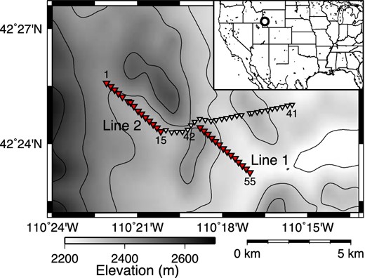
Geometry of receivers (triangles). We use receivers shown by red triangles for this study. Survey lines 1 and 2 contain receivers 1–15 and 42–55, respectively. The circle on the inset shows the location of the magnified area. The grey scale illustrates topography.
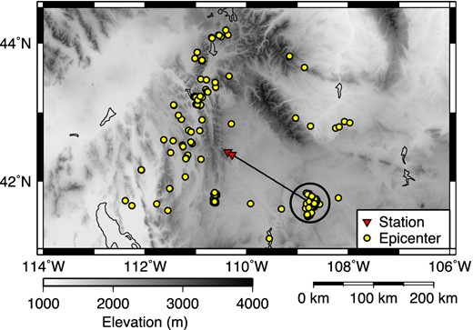
Geometry of earthquakes (yellow dots) and receivers (red triangles). We use an earthquake cluster (embraced by black circle) for the interferometry study. Triangles indicate the locations of receivers No. 1 and 55. The black line illustrates the great circle between the centre of the earthquake cluster and receiver No. 55. The grey scale illustrates topography.
Using this data set, several studies obtain images and/or velocities of the subsurface in the survey area. Leahy et al. (2012) apply receiver function to teleseismic events to image the subsurface. Schmedes et al. (2012) and Biryol et al. (2013) apply earthquake tomography to teleseismic and local earthquake data, respectively. Behm et al. (2014) apply seismic interferometry to reconstruct surface waves using traffic-induced noise and obtain Rayleigh- and Love-wave velocities. With teleseismic data, Behm & Shekar (2014) obtain shallow images from vertically incident reflected waves by employing blind deconvolution.
3.2 Observed data
Because the wavefield decomposition in Section 2 is valid for the wave propagation in a vertical plane, we restrict ourselves to hypocentres and receivers near the vertical plane. We use a cluster of earthquakes (represented by the black circle in Fig. 3), which contains about 100 earthquakes and produces quasi-plane waves with nearly the same angles of incidence. This cluster of earthquakes is 180 km away from the stations and located on the extensions of survey lines 1 and 2 in Fig. 2 (see the black line in Fig. 3). Therefore in this study, we use this cluster of earthquakes and receivers of survey lines 1 and 2 (the red triangles in Fig. 2) to reconstruct direct and reflected plane waves with seismic interferometry.
Fig. 4 shows sample observed wavefields excited by one earthquake. Direct P waves arrive around 28 s, S waves around 50 s, and surface waves around 70 s. Wavefields at receivers 29–30 are contaminated by traffic noise which is generated from a road close to these receivers. The high-energy waveforms contain frequencies up to 7 Hz. Because the aperture of the receiver array is small, we cannot accurately interpret seismic phases of each arriving wave from the move out of traveltimes in Fig. 4. Seismic phases of incoming waves comprise refracted waves from the crust (Pg, Sg), reflected waves from the crust-mantle boundary (Moho) (PmP, SmS), and refracted waves from the uppermost mantle (Pn, Sn). Note that we can apply seismic interferometry to any types of phases and we do not have to specify the seismic phases because we are interested in reflected waves from the shallow crust below the receiver array, and all seismic phases can produce these waves. Some studies use specific seismic phases to confine the angle of incident waves (e.g. Ruigrok et al.2010; Ruigrok & Wapenaar 2012). In this study, we estimate the traveltimes of each seismic phase to validate our interferometric wavefields, where we evaluate whether the reconstructed waves with seismic interferometry are reflected waves or later phases. To estimate traveltimes and relative amplitudes of each phase, we construct a local 3-D subsurface model based on Gans (2011) that includes crustal inhomogeneity and perform 3-D ray tracing with the program ANRAY (Pšenčík 1998). Results from ray tracing suggest that traveltime differences are very small for Pn/Pg as well as Sn/Sg, and PmP/SmS arrive 0.7/1.2 s later than Pn/Sn. At this offset, amplitudes of Pg/Sg are smaller than Pn/Sn and PmP/SmS. Although both traveltimes and, in particular, amplitudes still depend on the subsurface model, we conclude that the observed first arrivals are most likely Pn/Sn or PmP/SmS since their amplitudes are expected to be stronger than amplitudes of Pg/Sg waves.
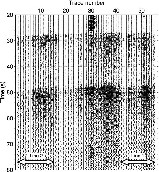
Example of observed records from an earthquake in the north–south horizontal component after applying a bandpass filter, 0.4–0.5–7–9 Hz. Time 0 s is the origin time of the earthquake. Trace numbers correspond with the receiver numbers in Fig. 2. The white arrows show the receivers used for survey lines 1 and 2.
3.3 Wavefield decomposition
To apply wavefield decomposition in the wavenumber–frequency domain using eq. (11), we need traces at uniform spatial intervals. Therefore, we interpolate the observed data in space using a spline interpolation before the decomposition. Note that the receiver intervals in survey lines 1 and 2 are almost uniform and the interpolation distances are small. Fig. 5 shows the interpolated wavefields after rotating the horizontal components in the radial direction (the same direction as the receiver lines).
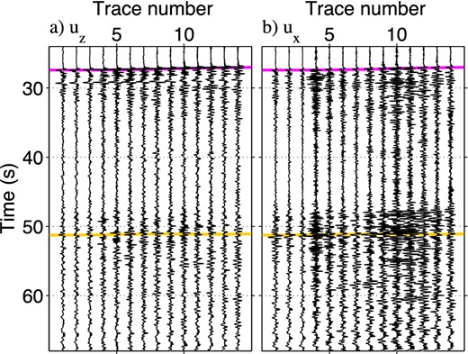
Space-interpolated observed record in (a) vertical and (b) radial components in line 1 (after rotating the horizontal components into the radial direction) from the same earthquake used in Fig. 4. Trace number is assigned after the space interpolation, and traces 1–14 correspond to receivers 42–55 in Fig. 4. We apply the same bandpass filter used in Fig. 4 to waveforms in all panels. The pink and yellow lines indicate the picked arrival times for the largest energy of direct P and S waves, respectively. Amplitudes are normalized individually at each panel.
Fig. 6 shows the particle motion around the P- and S-wave arrival times. We compute the angles of incident P and S waves by ray tracing with a velocity model based on Gans (2011); the angles of incidence in survey line 1 are 35° and 18° for P and S waves, respectively (the blue lines in Fig. 6). The particle motions around the P-wave arrivals correspond to the angle of incidence estimated by ray tracing, but the particle motions around S-wave arrivals do not. These particle motions do not show a clear pattern, which may be caused by the fact that S waves overlap with the P-wave coda, the S-wave arrival time is less clear than the P-wave time (see Fig. 5), and the subsurface may create strong PS converted waves (which we discuss later). Note that in both P and S waves, the particle motions do not have to perfectly align to the angle of incidence estimated by ray tracing because the incoming waves are not perfect plane waves and the velocity model for the ray tracing has some uncertainties.
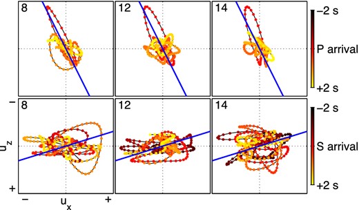
Particle motion of observed wavefields in the vertical and radial components (Fig. 5) at around (top row) P- and (bottom row) S-wave arrivals after applying the same bandpass filter used in Fig. 4. Red (0 s in the colour bar) indicates the times at the pink line for P waves and the yellow line for S waves in Fig. 5. Blue lines illustrate the particle motion based on the angle of incidence estimated by ray tracing. Top-left numbers at each panel describe trace numbers of each motion.
Wavefield decomposition shown in eq. (11) requires P- and S-wave velocities. We do not need to know the angle of incidence for the wavefield decomposition because we solve eq. (11) in the wavenumber–frequency domain. To estimate velocities, we employ the method proposed in Section 2 and minimize upgoing P-wave amplitude around S-wave arrival times as well as upgoing S-wave amplitude around P-wave arrival times. Fig. 7 shows upgoing/downgoing P/S waves decomposed from waves in Fig. 5 with estimated P- and S-wave velocities, which are 3.5 and 1.2 km s−1, respectively. Based on these velocities and an angle of 35° of the P incident wave, the reflection coefficients at the free surface are −0.905 (ṔP̀), 0.665 (ṔS̀), 0.273 (ŚP̀) and 0.905 (ŚS̀) (Aki & Richards 2002). In Fig. 7(a), the amplitudes in the pink/blue time intervals are larger than the yellow/green time intervals. In contrast in Fig. 7(b), amplitude differences between the pink/blue and yellow/green time intervals are not clear, which implies that the wavefields include strong PS converted waves in the pink/blue time interval.
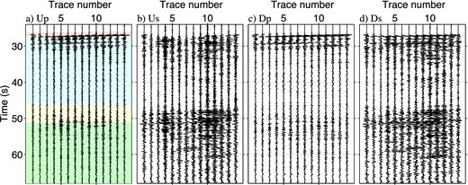
Upgoing/downgoing P/S waves after applying wavefield decomposition (eq. 11) to the wavefields in Fig. 5. We employ the same bandpass filter used in Fig. 4 in all panels. The colours in panel (a) indicate the time windows we use in this study to separate direct (pink for P and yellow for S) and reflected waves (blue for P and green for S). The arrival times represented by the pink and yellow lines in Fig. 5 locate the interfaces between pink/blue and yellow/green, respectively. Amplitudes are normalized separately at each panel.
Figs 8 and 9 show comparisons of wavefields and particle motions between upgoing P and S waves. In Fig. 8(a), because direct P waves (at around 27–27.5 s) exist only in the upgoing P wavefields, we successfully separate observed waves into upgoing P and S waves (see also the top row of Fig. 9). Strong upgoing S waves appearing just after the direct P waves in Fig. 8(a) indicate that the observed waveforms include strong PS converted waves. Since Fig. 8(b) is mostly red, upgoing S wavefields are dominant in this time interval, which implies that we can also separate wavefields in this interval. The particle motions in the bottom row of Fig. 9 are aligned along the horizontal blue lines, which denote that upgoing S wavefields are dominant in this interval. The anomalous particle motion in trace 14, which is at the edge of the array, may be caused by the space–wavenumber Fourier transform; therefore, we only use traces 3–12 for interferometry.
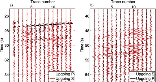
Comparison between upgoing P and S wavefields in Figs 7(a) and (b) at around (a) P-wave and (b) S-wave arrival times. Although in both panels upgoing P and S waves are shown in black and red, respectively, we change the order of wavefields for a display purpose; upgoing P is back and upgoing S is front in panel (a) and vice versa in panel (b). Amplitude ratios between upgoing P/S waves are preserved.
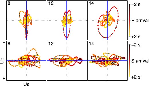
Particle motion of upgoing P and S wavefields at around (top row) P- and (bottom row) S-wave arrivals after applying the same bandpass filter used in Fig. 4. Red (0 s in the colour bar) indicates the times at the pink line for P wave and the yellow line for S waves in Fig. 5. Blue lines illustrate the ideal particle motion of P (top row) and S (bottom row) waves in the case when wavefields are perfectly separated and no converted waves are generated. Top-left numbers at each panel describe trace numbers of each motion. Note that in contrast to Fig. 6, the axes denote the upgoing P- and S-wave components.
4 APPLICATION OF SEISMIC INTERFEROMETRY TO EARTHQUAKE DATA
We introduce a mathematical description of seismic interferometry related to this study while assuming 2-D wave propagation and show reconstructed waveforms from the earthquake data. More information for seismic interferometry is given by Snieder et al. (2009) and Wapenaar et al. (2010a,b, 2011b), who summarize trace-by-trace and multi-dimensional interferometry. In this section, all equations are written in the space-frequency domain.
4.1 Trace-by-trace deconvolution
For trace-by-trace deconvolution interferometry, we compute deconvolution for each pair of traces at each earthquake. This method works well in the case of 1-D wave propagation (Snieder & Şafak 2006; Nakata & Snieder 2012) and can be applied to higher dimensions (e.g. Vasconcelos & Snieder 2008b).
4.1.1 Deconvolution without wavefield decomposition
In Fig. 10, we show averaged deconvolved wavefields over all earthquakes after applying trace-by-trace deconvolution to observed wavefields (eq. 12). Receiver A in eq. (12) is at offset 0 km (virtual source). The deconvolved wavefields in Fig. 10 are contaminated by noise around the zero-lag time; hence, trace-by-trace deconvolution using neither wavefield decomposition nor time windowing does not provide useful information about the subsurface.
Wavefields at line 1 obtained by applying trace-by-trace deconvolution to observed vertical (black) and radial (red) components (eq. 12). We apply a bandpass filter 0.4–0.5–7–9 Hz to wavefields in the vertical component and 0.4–0.5–4–6 Hz to wavefields in the radial component. Offset 0 km is the location of the virtual source.
4.1.2 Direct-wave extraction
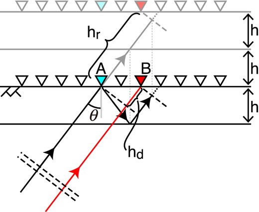
Schematic plane-wave propagation. Receivers (triangles) are deployed at the free surface (indicated by |$\rightthreetimes \rightthreetimes$|), and a plane wave (the black arrow at lower-left) propagates with angle θ of the incidence. Dashed lines, all of which are parallel, indicate the portions of plane waves. The red arrow illustrates the ray path for the different portion of the same plane wave as the black arrow. The model contains one horizontal layer and a half space below the layer. The thickness of the layer is h. Grey lines and receivers show unfolded imaginary layers and receivers to understand reflected plane waves based on Snell's law. Distance hd corresponds with the difference of the travel distance between direct upgoing waves to receivers A and B, and hr is the travel distance of the reflected waves from A to B. We do not show converted waves in this figure.
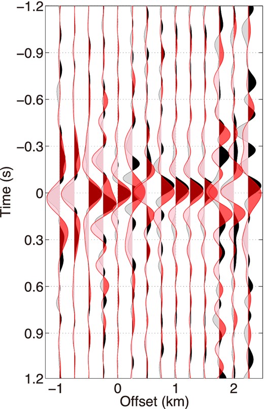
We apply trace-by-trace deconvolution (eq. 14), where we compute Up(B)/Up(A) and Us(B)/Us(A), to decomposed wavefields obtained from each earthquake and average over all earthquakes used (Fig. 12). The solid lines in Fig. 12 show the dips which maximize the amplitudes of slant-stacked waveforms. These dips depend on the angles of incidence and the wave velocities. Based on the angles of incidence estimated by ray tracing (35° for P waves and 18° for S waves), the P- and S-wave velocities are 4.2 and 1.5 km s−1, respectively. These velocities are average velocities over ray paths of the direct waves (hd in Fig. 11). We also apply this deconvolution to survey line 2 (dashed lines in Fig. 12). The dips in line 2 are flatter than in line 1, which corresponds to a high-velocity layer under line 2 (Leahy et al.2012). Note that without wavefield separation, we cannot clearly reconstruct direct waves (compare Fig. 10 with Fig. 12). The wavefield separation plays an important role for reconstructing waveforms with seismic interferometry.
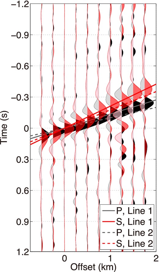
Wavefields in survey line 1 obtained by applying trace-by-trace deconvolution to upgoing P (black) and S (red) waves (eq. 14). The solid lines show the dip of P (black) and S (red) plane waves in survey line 1, and the dashed lines in survey line 2. We apply the same bandpass filters used in Fig. 10. Offset 0 km is the location of the virtual source.
4.1.3 Reflected-wave extraction
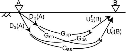
Relationship of upgoing/downgoing P/S wavefields and Green's functions between receivers A and B. The free surface is indicated by |$\rightthreetimes \rightthreetimes$|. The direction of arrows represents the direction of causality. Upgoing waves are reflected waves (direct upgoing waves are not shown).
We compute eq. (16) to obtain PP reflected waves and similar equations for PS, SP and SS reflected waves while applying time windowing for separating direct and reflected waves. We independently create time windows for each earthquake based on manually picking arrivals of each wave, and the time windows shown in Fig. 7(a) are the windows for the earthquake in Fig. 7. When we compute eq. (16) for each earthquake, we use only direct downgoing P waves [|$D^d_p(A)$|] instead of using entire downgoing waves [Dp(A)] to focus on the first-order surface related multiples as following the technique shown in Mehta et al. (2007). With this time window to isolate direct downgoing waves, we may create non-physical reflections caused by insufficient cancellation compared with using the full wavefields (appendix B in Ruigrok 2012). In our data, however, this time-gating technique increases the signal-to-noise ratio of deconvolved wavefields.
Fig. 14 shows all P/S combinations of the trace-by-trace deconvolved waveforms after averaging over all earthquakes used. For a display purpose, we show only one receiver gather (at trace 5), but we can compute all combinations of virtual sources and receivers. In Figs 14(a) and (b), we employ the pink/blue time windows shown in Fig. 7(a) (modified for each earthquake), respectively. Similarly, in Figs 14(c) and (d), we use the yellow/green time windows shown in Fig. 7(a) (modified for each earthquake). We apply cosine tapers at the edge of each time window. Although each panel in Fig. 14 aims to show the target reflected Green's function (e.g. Gpp for Fig. 14a), each panel includes unwanted crosstalk caused by the last term in eq. (16). Evaluating the amount of crosstalk is difficult, but we expect that the energy of SP reflected waves should be smaller than other reflected waves in the estimated angle of incidence (Aki & Richards 2002); for example in the assumption of horizontal layers, when the P and S velocities in the first/second layers are 3.5/5.0 and 1.2/2.2 km s−1 (modified after Leahy et al.2012) and the angle of P-wave incidence is 35°, the reflection coefficients at the interface are 0.189 (ṔP̀), −0.135 (ṔS̀), −0.055(ŚP̀), and −0.162 (ŚS̀). Almost no P-wave energy is present in Fig. 8(b), which also indicates that Gsp is small. However, the amplitudes in Fig. 14(c) are larger than those in Fig. 14(d), which might be caused by the crosstalk between downgoing P and S waves in eq. (16).
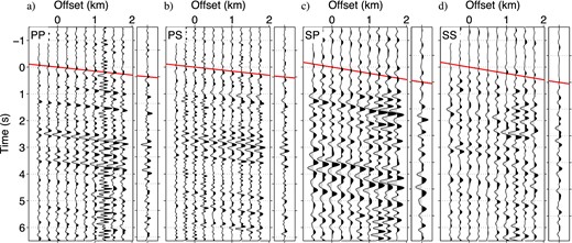
Reflected plane waves retrieved by trace-by-trace deconvolution. We compute (a) |$U^r_p(B)/D^{d}_p(A)$| (≈Gpp), (b) |$U^r_p(B)/D^d_s(A)$| (≈Gps), (c) |$U^r_s(B)/D^{d}_p(A)$| (≈Gsp) and (d) |$U^{r}_s(B)/D^{d}_s(A)$| (≈Gss). Each panel shows a receiver gather, and offset 0 km indicates the location of the common receiver. We apply bandpass filters with (a, b) 0.4–0.5–7–9 Hz and (c, d) 0.4–0.5–4–6 Hz. Red lines illustrate the dip for slant stacking, and the rightmost trace at each panel is the stacked trace. The amplitudes in panels (c, d) are multiplied by a factor 2.5 compared with those in panels (a, b), and the amplitudes in panels (a, b) are the same.
The right-most trace at each panel in Fig. 14 shows slant-stacked wavefields, where the dip for stacking (the red lines in Fig. 14) is chosen to maximize the peak amplitude of stacked waveforms. Since the dips are related to the wave velocities and the angles of incidence, the dips in Figs 14(a) and (b) as well as those in Figs 14(c) and (d) are almost the same. Stacked waveforms in Fig. 14 are noisy and difficult to interpret.
4.2 Trace-by-trace cross-coherence
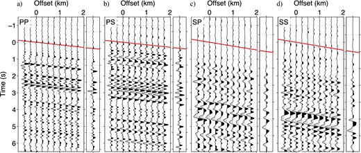
Reflected plane waves retrieved by trace-by-trace cross-coherence. We compute (a) |$U^{r}_p(B)D^{d*}_p(A)/|U^{r}_p(B)||D^{d}_p(A)|$| (≈Gpp), (b) |$U^{r}_p(B)D^{d*}_s(A)/|U^{r}_p(B)||D^{d}_s(A)|$| (≈Gps), (c) |$U^{r}_s(B)D^{d*}_p(A)/|U^{r}_s(B)||D^{d}_p(A)|$| (≈Gsp) and (d) |$U^{r}_s(B)D^{d*}_s(A)/|U^{r}_s(B)||D^{d}_s(A)|$| (≈Gss). Each panel shows a receiver gather, and offset 0 km indicates the location of the common receiver. We apply the same bandpass filters as used in Fig. 14. Red lines illustrate the dip for slant stacking, and the rightmost trace at each panel is the stacked trace. The amplitudes in panels (c, d) are multiplied by a factor 2.5 compared with those in panels (a, b), and the amplitudes in panels (a, b) are the same.
4.3 Multidimensional deconvolution
Because MDD treats the extraction of the Green's function as an inverse problem, MDD has several advantages compared with trace-by-trace interferometry. MDD can be applied to passive seismic data generated by unevenly distributed sources in a dissipative medium (but MDD requires evenly distributed receivers) (van der Neut et al.2011b; Wapenaar et al.2011a,b). Snieder et al. (2009) suggest that one can retrieve Green's functions without estimating source spectra by using MDD. This method also removes complicated overburden without requiring a velocity model when receivers are embedded inside a medium (van der Neut et al.2011a,b). Note that by comparing eqs (16) and (22), MDD retrieves the Green's functions without unwanted crosstalk when we separate P and S waves.
Fig. 16 shows wavefields reconstructed by MDD interferometry (expression 22). We again apply time windows to downgoing waves to isolate direct waves for increasing the coherency of deconvolved wavefields. For MDD interferometry, we also have a possibility to create pseudo reflections with applying these time windows (Ruigrok 2012). The amplitudes of the acausal waves are weaker than those in Figs 14 and 15, which indicates that based on the criterion of causality the quality of wavefields produced by MDD is better than trace-by-trace interferometry. Wavefields in Fig. 16 do not include unwanted crosstalk, which contaminates waveforms in Figs 14 and 15, because MDD solves the inverse problem (eq. 22). As shown in Fig. 8(b), SP converted waves are weak [compare Fig. 16(c) with the other panels in Fig. 16]. Also, the slant-stacked wavefields in Figs 16(c) and (d) are more dissimilar than the wavefields in Figs 15(c) and (d) obtained by trace-by-trace cross-coherence. This is an indication that MDD successfully eliminates the crosstalk that contaminates Figs 15(c) and (d).
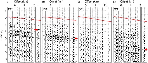
Reflected plane waves retrieved by multidimensional deconvolution. (a) Gpp, (b) Gps, (c) Gsp and (d) Gss. Each panel shows a receiver gather, and offset 0 km indicates the location of the common receiver. We apply the same bandpass filters as used in Fig. 14. Red lines illustrate the dip for slant stacking, and the rightmost trace at each panel is the stacked trace. The red arrows on the rightmost traces in panels (a, b, d) point at the waves that we interpret. The amplitudes in panels (c, d) are multiplied by a factor 2.5 compared with those in panels (a, b), and the amplitudes in panels (a, b) are the same.
Leahy et al. (2012) show that a subhorizontal basement is located at about 3.8 km depth. The waves pointed by the three arrows in Fig. 16 are possibly reflections from the basement; their arrival times are 1.38 s (PP), 2.66 s (PS) and 4.10 s (SS). We do not pick the SP reflected wave because it has low signal-to-noise ratio. These arrival times are much larger than the estimated traveltime differences between Pn/Sn and PmP/SmS, which are 0.7 and 1.2 s. Although the differences of the traveltimes estimated by ray tracing include some uncertainties due to the subsurface model used for the ray tracing, we conclude that the retrieved waves are reflected waves but not later direct arrivals based on two reasons explained below. First, the arrival times of these reflected waves highlighted by the arrows in Fig. 16 are dependent. Using the arrival times of the PP and SS reflected waves, the arrival time of the PS reflected wave should be 2.74 s, which is a 3 per cent discrepancy [≈(2.74 − 2.66)/2.66] from the observed time in Fig. 16(b). Second, the large difference of PP and SS arrival times in Fig. 16 indicates large Vp/Vs ratio, which is the condition of near surface. Therefore, the arrival times obtained from Fig. 16 include near-surface information. When we assume that the reflector is flat, the average P and S velocities over the ray paths of the reflected waves (hr in Fig. 11) are 4.5 and 1.7 km s−1, respectively, with the angles of incidence we estimated.
5 DISCUSSION OF VELOCITIES
The estimated velocities (4.2 and 1.5 km s−1 from direct waves, and 4.5 and 1.7 km s−1 from reflected waves) and velocities used for the wavefield decomposition (3.5 and 1.2 km s−1) are different. These differences indicate the depth variation of velocities. Gans (2011) and Leahy et al. (2012) show that the velocities in the region of survey line 1 monotonically increase with depth. The velocities estimated from direct (from Fig. 12) and reflected waves (from Fig. 16) are the average velocities over the distances hd and hr in Fig. 11. Based on the estimated angles of incidence and the depth of the reflector, the velocities from the reflected waves include the information of deeper structure than the direct waves. Therefore, the fact that the estimated velocities from reflected waves are faster than those from direct waves is consistent with previous studies. The velocities used for decomposition are theoretically the velocities at the surface but practically the average velocities over a medium with some thickness depending on the wavelength we used. Since the velocities used for decomposition are lower than the velocities estimated from direct waves, the decomposition is sensitive for the near-surface structure shallower than the depth of hd cos (θ) in Fig. 11 for the used frequency range.
6 CONCLUSIONS
We apply seismic interferometry to plane waves excited by a cluster of earthquakes and obtain subsurface information on a local scale. To improve the quality of interferometric wavefields, we employ several techniques such as upgoing/downgoing P/S wavefield decomposition, time windowing to separate direct and reflected waves, and multidimensional analysis. The wavefield decomposition proposed here works well when the medium has no or weak lateral heterogeneity. For trace-by-trace interferometry, wavefield decomposition enhances coherence of interferometric wavefields between traces. We retrieve the Green's matrix without unwanted crosstalk of P and S waves with MDD interferometry. Although MDD interferometry requires wavefield separation, the computed waveforms follow causality and have the highest signal-to-noise ratio compared with trace-by-trace interferometry. The difference between the velocities estimated from direct waves and reflected waves retrieved by seismic interferometry is evidence of the depth variation of the velocities.
We are grateful for financial support from ExxonMobil and the sponsor companies of the Consortium Project on Seismic Inverse Methods for Complex Structures at the Center for Wave Phenomena. We thank the IRIS data management centre and ExxonMobil to provide the earthquake data, and USGS and ANF for managing the earthquake catalog. Figs 2 and 3 are produced by using the Generic Mapping Tools (GMT: http://gmt.soest.hawaii.edu, last accessed July 2014). We thank Filippo Broggini and Joost van der Neut for their professional help to implement seismic interferometry, and to Kees Wapenaar and Deyan Draganov for their valuable reviews.
