Complexity of the rupture process during the 2009 L'Aquila, Italy, earthquake

Summary

1 Introduction

The M_w 6.1 L'Aquila main shock is one of the best-recorded normal faulting earthquakes worldwide and has allowed the collection of an extremely interesting observational data set. It occurred on 2009 April 6 (01:32 UTC) and struck the Abruzzi region in central Italy (see Fig. 1) causing more than 300 fatalities in the L'Aquila City and nearby villages. The availability of high-quality data set (including strong motion accelerograms, GPS, CGPS and Differential Synthetic Aperture Radar Interferometry—DInSAR—measurements) promoted numerous studies to constrain the rupture process. The L'Aquila main shock ruptured a ∽16-km-long, ∽50° SW-dipping normal fault located in the extensional tectonic setting of central Apennines (Chiarabba et al. 2010; Chiaraluce et al. 2011a). Different studies have pointed out the complexity of the earthquake nucleation (Lucente et al. 2010), the initial stages of the rupture history (Ellsworth & Chiaraluce 2009; Di Stefano et al. 2011) and the subsequent coseismic rupture propagation (Cirella et al. 2009). Scognamiglio et al. (2010) have discussed the different magnitude estimates between the regional Centroid Moment Tensor (CMT; M_w 6.3, Pondrelli et al. 2010) and the Time-Domain Moment Tensor (TDMT, M_w 6.1) solutions.

Figure 1

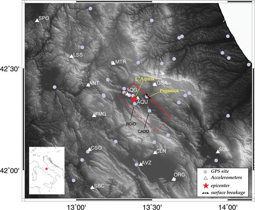
Map of the fault geometry of the 2009 L'Aquila earthquake. The red box represents the surface projection of the fault plane adopted in this study. White triangles represent the selected strong motions stations. Violet dots represent the GPS sites; the red star indicates the epicentre. In yellow are displayed the location of the L'Aquila town and Paganica village.

Open in new tabDownload slide

The coseismic slip pattern imaged by inverting strong motion waveforms and GPS displacements reveals a heterogeneous slip distribution on the fault plane characterized by two main slip patches: the largest and deeper one is located 8 km from the hypocentre southeastwards along the strike, while the shallower is located a few kilometres updip from the hypocentre (Cirella 2009; Cheloni et al. 2010; Scognamiglio et al. 2010). The inversion of DInSAR data provides consistent results, although it concentrates most of slip on the main deep slip patch (Atzori et al. 2009; Trasatti et al. 2011). Moreover, numerous studies confirm that along-strike rupture directivity characterizes the observed ground motions (Pino & Di Luccio 2009; Akinci et al. 2010) and relatively high acceleration amplitudes were recorded at strong motion receivers on the hangingwall of the main fault (Ameri et al. 2009; Celebi et al. 2010), where the L'Aquila town is located.

Despite its moderate magnitude, the rupture process of the L'Aquila main shock is surprisingly complex. The analysis of the closest strong motion accelerograms shows an initial emergent P-wave signal (hereinafter EP) followed by an impulsive onset (IP) after few tenths of second (Michelini et al. 2009). This suggests that the initial stages of the rupture are characterized by a relatively small moment release (initiated by the EP) followed ∽0.9 s later by a high moment release (beginning with the impulsive phase, IP) located nearly 2 km updip from the hypocentre (Di Stefano et al. 2011). The rupture history imaged by Cirella et al. (2009) also displays this initial updip propagation. Moreover, afterslip has been geodetically measured and located in the shallow SE border of the main shock fault plane (Cheloni et al. 2010), where almost no coseismic slip has been inferred. These observations and modelling results together with the interpretation of fluid involvement in the foreshock activity and the earthquake nucleation process (Lucente et al. 2010) corroborate the heterogeneity of the rupture process during the L'Aquila main shock.

The aim of this study is to further investigate these issues by imaging the rupture history through the inversion of strong motion, GPS and DInSAR data (inverted either separately or jointly). To address the problem of the heterogeneity of the rupture process, we give particular attention to the variability of model parameters and we attempt to better constrain the local rupture velocity on the fault plane. To accomplish these tasks we have used a modified version of Piatanesi's et al. (2007) inversion algorithm (see details in Section 4).

2 Data

The 2009 L'Aquila main shock has allowed the collection of an excellent data set for a moderate-magnitude normal faulting earthquake. In this work we have analysed and inverted strong motion, GPS and DInSAR data to image the coseismic rupture on the fault plane.

2.1 Seismological data

The main shock and its largest aftershocks have been recorded by several digital stations of the Italian strong-motion network (‘Rete Accelerometrica Nazionale’, RAN) managed by the Italian Civil Protection (http://itaca.mi.ingv.it/ItacaNet), by several broad-band stations and accelerometers of the MedNet network (http://mednet.rm.ingv.it/data.php) and by the digital permanent seismic stations of the Italian National Seismic Network (INSN) managed by Istituto Nazionale di Geofisica e Vulcanologia (INGV; http://iside.rm.ingv.it/iside/standard/index.jsp). Immediately after the main shock, the INGV and the Laboratoire de Géophysique Interne et Tectonophysique (LGIT) of Grenoble (France) deployed a dense temporary seismic network of 40 digital seismic stations (Chiaraluce et al. 2011a), which allowed the recordings of the whole aftershock sequence. Detailed aftershock locations enable the identification of the main shock fault plane and to constrain the fault geometry (Di Stefano et al. 2011).

In this study we have selected 13 three-component digital accelerometers of the RAN Network and the AQU (MedNet) accelerogram (see Fig. 1). They were integrated to obtain ground velocity time histories and bandpass filtered between 0.02 and 0.5 Hz with a two-pole and two-pass Butterworth filter. We do not model higher frequencies because of difficulties in computing appropriate Green's functions and to reduce bias caused by site effects, that are affecting ground motion time histories at frequencies higher than 0.6 Hz (De Luca et al. 1998).

2.2 GPS data

To image the details of the slip distribution through the inversion of GPS data, we have considered 36 three-component GPS displacements inferred from measurements at the closest receivers (see Fig. 1) deployed by different agencies (see Table 1). These horizontal and vertical coseismic displacements represent a subset retrieved from the analysis of the 43 GPS measurements published by Cheloni et al. (2010; see their tables S1 and S2).

Table 1

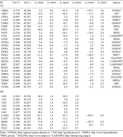
(A) Coseismic offset from continuous GPS measurements; (B) coseismic offset of survey-style GPS sites used in this study. A_e, A_n and A_u are east, north and vertical components in mm, while S_e, S_n and S_u are east, north and vertical one-sigma associated uncertainties.

Open in new tabDownload slide

In particular, to ensure good azimuthal coverage around the fault and to consider a high signal-to-noise ratio (>1), we have selected 25 coseismic offsets from permanent GPS sites (Table 1A) and 11 survey-style GPS benchmarks (Table 1B), three of which (CADO, ROIO and SELL) are survey-mode sites installed 4 d before the main shock (Anzidei et al. 2009). We have used the data processed by Cheloni et al. (2010). These authors mapped the displacements with respect to CESI station (INGV Network), which is located 80 km northwest from the epicentre and that did not display any coseismic offset and has negligible secular motion relative to the stations near the epicentre (D'Agostino et al. 2008).

In this study, we have inverted a more complete and updated GPS data set with respect to Cirella et al. (2009). This guarantees a better spatial resolution (azimuthal coverage) of the fault plane, in particular on the southeastward portion of the causative fault.

2.3 DInSAR data

We have applied the DInSAR technique to the Envisat and ALOS SAR satellite data. The ENVISAT pair has been acquired on 2008 April 27 and 2009 April 12 from the descending orbit with a look angle of 23° and a perpendicular baseline of 41 m; while the ALOS pair has been taken on 2008 July 20 and 2009 April 22 from the ascending orbit with a look angle of 36° and a perpendicular baseline of 322 m. Both interferograms have been generated at ∽300 m resolution, to achieve a sufficient spatial resolution and an acceptable signal-to-noise ratio. Moreover, the 90 m SRTM digital elevation model is used to subtract the topographic contribution. In the resulting ENVISAT C-band differential interferogram (Fig. 2a) each colour cycle (fringe) corresponds to a ground displacement of ∽ 2.8 cm along the line of sight (LoS) of the satellite, while in the ALOS L-band each fringe corresponds to an ∽11.8 cm in LoS (Fig. 2b). It is worth noting that the bigger wavelength of L-band system with respect to C-band results in lower temporal decorrelation and in longer critical baselines, providing more coherent interferograms (i.e. the complex correlation value of two SAR images; Chini 2010). To reduce the interferometric phase noise an adaptive filter has been applied (Goldstein & Werner 1998) to both interferograms, while a Region Growing approach has been used for obtaining the unwrapped DInSAR maps (Reigber & Moreira 1997).

Figure 2

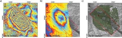
(a) Envisat wrapped interferogram; (b) ALOS wrapped interferogram; (c) Green colour shows the 4599 resampled pixels (size 300 m), from both interferograms, selected in this study. The red rectangle represents the surface projection of the fault plane fixed for this study, while the red star represent the epicentre.

Open in new tabDownload slide

The coseismic ground displacement of the L'Aquila earthquake has also been measured by L-, C- and X-band DInSAR interferograms, and a very good agreement has been found in all the different data sets, indicating that the presence of atmospheric artefacts was limited (Stramondo et al. 2011). Despite the time interval spanned by the pre- and post-seismic images for both interferograms is quite long (nearly a year), we can assume that, within this interval, the inferred deformation pattern is caused by coseismic slip because post-seismic deformation is negligible (Lanari et al. 2010; Reale et al. 2011; Stramondo et al. 2011; Chini 2012) and pre-seismic transients are absent (Amoruso & Crescentini 2010; Sansosti et al. 2010).

3 Model Setup

3.1 Crustal structure

For computing the Green's functions, we have assumed for all recording stations (except for AQU and AQG) the 1-D velocity model (nnCIA.mod) proposed by Herrmann et al. (2011), and calibrated during the sequence through the analysis of surface wave dispersion. For AQU and AQG seismic stations we have adopted a 1-D velocity model specific for these receivers obtained by the analysis of receiver functions (Bianchi et al. 2010). A relatively high velocity between 3 and 10 km depth and a wave velocity inversion below 10 km characterize this latter crustal model. The nnCIA.mod velocity model for both V_P and V_S and the V_S profile proposed by Bianchi et al. (2010) for AQU and AQG are shown in Fig. 3. P-wave velocity for the latter model has been derived from V_S by assuming a V_P/V_S ratio of 1.9, which is consistent with receiver function analyses and with the 3-D seismic tomography proposed by Di Stefano et al. (2011).

Figure 3

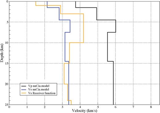
S- and P-velocity profiles adopted to compute the Green's function.

Open in new tabDownload slide

The kinematic tractions on the fault plane are calculated using the Discrete Wavenumber–Finite Element (DWFE) integration technique (Spudich & Xu 2003), which allows the computation of the complete response of a 1-D layered medium (Olson 1984; Spudich & Archuleta 1987). In their inversion attempts for the 2000 western Tottori earthquake Piatanesi (2007) included the effects of using different velocity models. Moreover, Yagi & Fukahata (2011) introduced the uncertainty of the Green's function into their waveform inversion and demonstrated that neglecting modelling errors, due to Green's function calculation, the inferred total slip vector can be unstable and opposite slip components might characterize the solution. However, we point out that the velocity models adopted in this study rely on results from distinct approaches (receiver functions, surface wave dispersion and crustal tomography) that used different data and reveal several common features (such as the shear wave velocity inversion at 10 km below L'Aquila). Therefore, although we cannot exclude that short wavelength complexities of slip pattern are due to limitations in modelling the wave propagation, we believe that the choice of the crustal model is not affecting the imaged key features of the rupture model in the adopted frequency band.

3.2 Fault model

The adopted fault plane, striking N133°E and dipping 54° to the SW (Cirella et al. 2009), is 28 km long and 17.5 km wide with the shallow top border located at 0.5 km depth just below the surface breakage observed along the Paganica Fault (EMERGEO WG 2010, Cinti et al. 2011; see Fig. 1). We assume the INGV hypocentre (Chiarabba et al. 2009). The strike of the fault is well constrained by DInSAR data (Atzori et al. 2009). Our assumed dip angle is slightly higher than that resulting from aftershock locations (∽50°, Di Stefano et al. 2011), but this difference lies within the uncertainties.

For these reasons, we have maintained the fault geometry used by Cirella et al. (2009). Alternative values for strike and dip angles proposed in the literature (e.g. Scognamiglio et al. 2010) so far lie within the associated uncertainties (±5°). The dip angle adopted in this study yield a fault plane whose shallowest tip is in agreement with observed surface breakages and the position of the Paganica Fault (EMERGEO WG 2010; Cinti et al. 2011). The difference between the hypocentre used in this study and the EP phase located by Di Stefano et al. (2011) and Michelini et al. (2009), ∽600 m, also lies within the uncertainties. We invert for slip direction, assuming a dominant normal fault mechanism consistent with moment tensor solutions (Pondrelli et al. 2010; Scognamiglio et al. 2010) and aftershocks focal mechanisms and allowing the rake angle to vary in the range 270°± 40°.

4 Methodology

4.1 Adopted technique

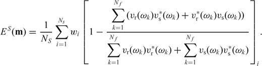
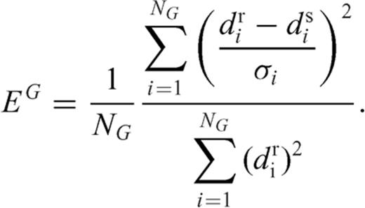
We use the two-stage non-linear technique described in Piatanesi et al.(2007) that allows the joint inversion of strong motion records and static displacements. We apply the same global optimization procedure to invert all the data sets, but we adopt different cost functions for the strong motion and geodetic data (see later and Piatanesi et al. 2007). This strategy reduces the effect of subjective choices and facilitates the comparison between single data sets and joint inversions. The extended fault plane is divided into subfaults with model parameters assigned at the corners, whereas the parameters within a subfault are allowed to vary through a bilinear interpolation of the nodal values. This implies that the convolution between computed tractions and source time function (STF) is calculated on a finer grid than that represented by the nodes where we infer model parameters. This will mitigate the effects of modelling errors due to the fault parametrization (Yagi & Fukahata 2008).

We adopt a single window approach where each point on the fault can slip only once following a prescribed functional form of the STF. Our technique has been implemented to allow the choice of different slip velocity STFs (Cirella 2008). In this study, the adopted STF is the regularized Yoffe function (Tinti et al. 2005) having a constant time to peak slip velocity (T_acc) equal to 0.225 s. Although the frequency bandwidth of the data used in this study does not allow to discriminate between different functional forms of the STF, our assumption is justified by the need of using a dynamically consistent slip-velocity function. We invert for four source parameters, which are spatially variable on the fault plane: peak slip velocity, slip direction, rupture time and rise time. The final slip distribution is computed from inverted model parameters (rise time and peak slip velocity) according to the assumed STF.

During the first stage (ensemble build-up), a heat-bath simulated annealing algorithm explores extensively the model space to generate an ensemble of models that efficiently sample the good data-fitting regions. All the explored models and their cost function values are then collected to build-up the model ensemble. To quantify the goodness of a model we choose a total cost function given by a weighted sum of the cost functions associated to the different data sets. According to Piatanesi et al. (2007), recorded and synthetic seismograms are compared in the frequency domain assuming a hybrid representation between L1 and L2 norms:

(1)

Here E^S(m) is the cost function corresponding to model m, N_s the number of seismograms, N_f the number of frequencies, v_r and v_s are, respectively, the recorded and synthetic ground velocity spectra, * symbol stands for complex conjugates, ω_k is the kth frequency of a ground velocity spectrum and ω is a relative weight to be assigned to each record. This cost function takes information from both the shape and the amplitude of a waveform and it turns out that it is more robust than standard least squares (Ji et al. 2002; Liu & Archuleta 2004).

For the GPS and DInSAR measurements we adopt a sum-squared (L2 norm) of the residuals between synthetic and recorded static displacements normalized to the observed data (see Cirella et al. 2008, for further details):

(2)

Here N^G is the number of GPS or DInSAR displacements, d^r and d^s are recorded and synthetic displacements, respectively, and σ is the error associated to the measured data. The cost function represents a measure of goodness of a model since it minimizes the misfit between observed and synthetic data (‘optimization’ process). In this study we use the cost function values as a measure of misfit.

In the second stage (‘ensemble appraisal’), the algorithm performs a statistical analysis of the whole model collection by selecting a subset (Ω) composed by those rupture models having a cost function value smaller than a given threshold. Finally, from the Ω subset, an average model and its standard deviation are computed.

We invert simultaneously for all the parameters at nodal points equally spaced (3.5 km) along strike and dip directions. During the inversion, we fix a given range of variability for each model parameter. In particular, in this study we adopt the following variability intervals: peak slip velocity values can range between 0 and 3.5 m s⁻¹ at 0.25 m s⁻¹ interval; the rise time between 0.75 and 3 s at 0.25 s interval and the rake angle from 230° to 310° in steps of 10°. The rupture time at each grid node is constrained by the arrival time from the hypocentre of a rupture front having a speed comprised between 1.4 and 4 km s⁻¹.

4.2 Check of local rupture velocity

When we assign minimum and maximum values for rupture velocity measured with respect to the hypocentre, we impose the range of variability of the rupture time parameter in each grid node. However, this does not impede to have locally extremely high rupture velocities (i.e. larger than P-wave velocity). To avoid unphysical conditions (such as acausality of the rupture front propagation), we have introduced in our procedure an additional constraint on the local rupture velocity.

During the second stage (appraisal) the inversion procedure selects all models having a cost function not exceeding 5 per cent of the minimum cost function value. This threshold has been selected both to have a small deviation from the minimum cost function and a reasonable number of source models belonging to selected Ω subset. Then, the algorithm checks for the values of local rupture velocity of each model belonging to the selected subset and discards all those models having a local rupture velocity larger than P-wave velocity. In this way, we can guarantee that the selected rupture models forming the Ω subset do not have acausal rupture propagation.

The local velocity is computed from the gradient of rupture times, following the procedure proposed by Pulido & Dalguer (2009) and Hok & Fukuyama (2011). To compute the local rupture velocity vectors at each point on the fault plane, we first evaluate the rupture slowness vectors, as the gradient of rupture times (t) along strike and dip directions (identified by unit vectors and ):

(3)

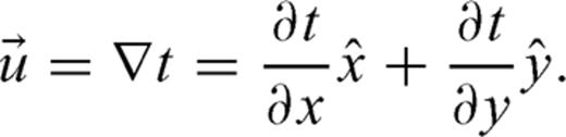
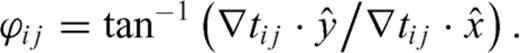
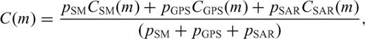
then, the rupture velocity vector , at each point on the fault identified by its position along the strike (i) and dip (j) directions is given by:

(4)

where ϕij is the angle between the rupture velocity vector and the fault strike direction

(5)

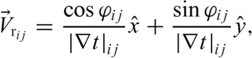
5 Single Data Set Inversion

5.1 GPS data inversion

We have first inverted the GPS displacements at the selected 36 receivers discussed earlier. The inferred slip distribution for the average model and the fit to the observed data are shown in Fig. 4. The imaged coseismic slip pattern is characterized by two main slip concentrations: the first slip patch is located at shallow depth just updip the rupture nucleation (the hypocentre), while the second is located southeastwards from the hypocentre between 7 and 11 km in the downdip direction. The Paganica surface breakages coincide with the deep slip patch and surprisingly they do not match the shallowest slip concentration imaged by GPS data (see Fig. 4).

Figure 4

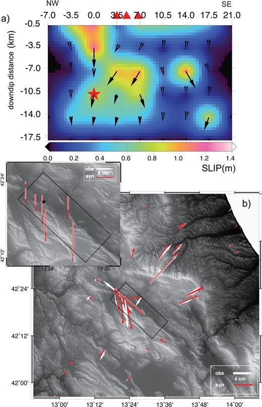
(a) Inverted rupture model of the 2009 L'Aquila earthquake retrieved from the inversion of the measured GPS; the panel shows the slip and rake distributions on the fault plane. Red triangles display the location of the Paganica surface breakages. (b) Comparison of measured (white arrows) with synthetic (red arrows) horizontal coseismic displacement (main panel); comparison of measured (white arrows) with synthetic (red arrows) vertical coseismic displacement (inset panel).

Open in new tabDownload slide

The retrieved slip distribution (Fig. 4a) is consistent with that one inferred by Cheloni et al. (2010), although in this study we invert a subset of the data used by these authors and we use a 1-D velocity model instead of a homogeneous half-space. We compute coseismic static deformations for a layered crustal structure from the zero frequency components of seismograms simulated through the Compsyn code (Spudich & Xu 2003). As explained in Piatanesi et al. (2007) and mentioned earlier, we invert geodetic displacements through the same inversion procedure used for strong motion data. The analysis of the misfit through the cost function values (see Table 2) allows us to conclude that the data are satisfactory matched, both for horizontal and vertical coseismic displacements (see Fig. 4b). Moreover, we point out that the average model yields a fit to the data comparable to that obtained through the best-fitting model (see their cost function values listed in Table 2), revealing that the appraisal stage performed in our inversion procedure is robust. In other words, averaging the selected slip models does not degrade the fit to the data. The slip direction shows some variability, in particular within the deep slip patch. The oblique slip direction is required to improve the fit to CADO and ROIO displacement vectors.

Table 2

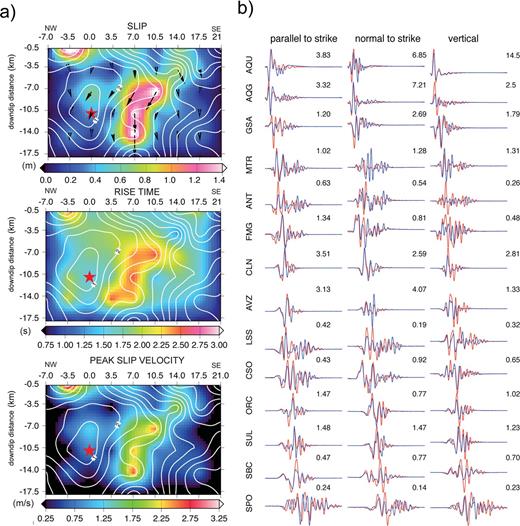
Cost function values resulting for the single data set and joint inversions and computed from the average and the best-fitting models. The shadowed values are obtained from the misfit resulting from forward modelling of GPS and DInSAR data using the source model of the single data set inversion (same row). The values annotated in bold indicates the cost functions for the best-fitting model identified by each inversion.

Open in new tabDownload slide

Our model obtained by inverting the GPS displacements suggests that the largest slip amplitude is located at shallow depth, on the shallower slip patch. However, the presence of peak slip amplitude at shallow depths is not consistent with the lack of surface ruptures on that portion of the fault as well as with the position of the observed surface breakages on the Paganica Fault. We will further discuss this feature in the following.

5.2 DInSAR data inversion

We have inverted the DInSAR interferograms shown in Fig. 2 (obtained from ENVISAT and ALOS SAR data), which represent the deformation along the LoS of the satellites. The looking angles of the two satellites are 23° and 36° for ENVISAT and ALOS, respectively, and we compute the synthetic deformation along the LoS direction. Considering the observation geometry of the two satellites used in this study, we emphasize that the horizontal component of measured deformation is negligible and/or below the data noise level (Stramondo et al. 2011), which in turn implies that DInSAR data contain information on vertical deformation.

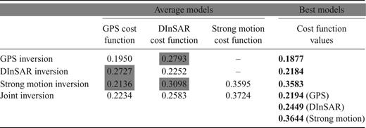
The slip distribution corresponding to the average model inferred by inverting DInSAR data is shown in Fig. 5(a). Fig. 5(b) displays the misfit between synthetic deformation and observations. The agreement between our model predictions and DInSAR data is quite satisfactory, as corroborated by the cost function's value listed in Table 2. The larger misfit on the southernmost shallow portion of the fault is likely due to possible complexities of fault geometry as well as to the presence of distributed deformation on a complex fault system (Chiaraluce et al. 2011b). Moreover this is an area not acquired by the ALOS satellite and characterized by a low coherence in the Envisat interferograms.

Figure 5

(a) Inverted rupture model of the 2009 L'Aquila earthquake retrieved from the inversion of the DInSAR data; the panel shows the slip and rake distributions on the fault plane. (b) Relative error between the observed and synthetic DInSAR displacement; black lines show slip contouring.

Open in new tabDownload slide

Consistently with previous results, the slip is concentrated in a main slip patch located at depths ranging between 3.5 and 10.5 km along the downdip direction, and nearly 6 km southeastwards along the strike direction. This slip model is quite similar to that obtained by Atzori et al. (2009). This deep slip patch is present in both slip models obtained by inverting GPS displacements (Fig. 4) and DInSAR data (Fig. 5) and it is located at similar depths. Although DInSAR data also suggest the presence of slip (∽50 cm) at shallow depths above the hypocentre, the amplitude and the spatial extension of this patch differs substantially from that imaged by inverting GPS data.

The difference between the slip models shown in Figs 4 and 5 likely depends on the different along-dip resolution of DInSAR and GPS data. The slip model inferred by inverting DInSAR data yields a poorer fit to GPS data than the model retrieved from GPS displacements (see Table 2). Similarly, the slip model inferred by inverting GPS data does not match DInSAR observations as the DInSAR model. This discrepancy might be also due to the fact that DInSAR data do not contain information on the observed horizontal deformation.

5.3 Strong motion data inversion

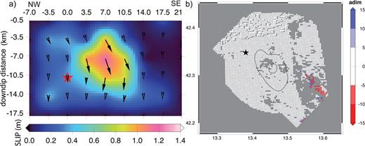
We have integrated ground acceleration time histories to obtain the ground velocity waveforms at the 14 sites shown in Fig. 1. The latter have been bandpass filtered between 0.02 and 0.5 Hz and inverted to image the rupture history during the L'Aquila main shock. The inferred distribution of model parameters and the fit to ground motion data are shown in Fig. 6, panels (a) and (b), respectively. The cost function's value for the average model is listed in Table 2. We remind here again that the slip distribution is calculated a posteriori from peak slip velocity and rise time according to the adopted STF (as explained earlier). Fig. 6(b) shows the fit to the three components of observed ground motion waveforms. The fit to the data is quite good with very few exceptions likely due to site effects and complex propagation paths.

Figure 6

(a) Inverted rupture model (average model from ensemble inference) of the 2009 L'Aquila earthquake retrieved from the inversion of the strong motion data. Upper, middle and bottom panels show total slip, rise time and peak slip velocity distributions, respectively. The rupture time is shown by contour lines in white colour at 1 s intervals; the black arrows displayed in top panel represent the slip vector. (b) Comparison of recorded strong motion (blue lines) with synthetic waveforms computed from the inverted rupture model (red lines). Numbers with each trace are peak amplitude of the observed waveforms in cm s⁻¹.

Open in new tabDownload slide

The source model retrieved by inverting strong motion data fits GPS data quite well, and much better than the DInSAR model (see Table 2). However, the strong motion model yields a poorer fit to DInSAR observations than the other models shown in Figs 4 and 5.

Nevertheless the rupture model imaged by solely inverting strong motion data contains features consistent with both GPS and DInSAR models. The coseismic slip is concentrated in two main slip patches: the main and deeper patch located between 6 and 10 km along the strike direction and the shallower slip concentration located updip with respect to the rupture nucleation. Therefore, the strong motion data inversion agrees with DInSAR data in locating the main slip patch at depth (both in terms of seismic moment and spatial extension), but it is also consistent with GPS data in suggesting a shallow slip patch updip the earthquake nucleation (although with less seismic moment and spatial extension).

The slip direction is consistent with the model inferred by inverting GPS data, suggesting dominant normal faulting with a minor right-lateral strike-slip component. The rupture times are quite heterogeneous and clearly reveal a complex rupture history.

6 Joint Inversion

Finally, we have performed the joint inversion of GPS, DInSAR and ground velocity time histories trying to extract the relevant features characterizing the rupture history during the L'Aquila main shock. The total cost function is computed through a weighted sum of the cost functions associated to the different data sets:

(6)

where p_i and C_i are the weight and the cost function for each data set (strong motion [SM], GPS and DInSAR); the latter depends on the selected rupture model (m). After several ‘trial-and-error’ tests, we have found that for the L'Aquila main shock it is reasonable to maintain the same weight for all data sets.

The inferred average rupture model is shown in Fig. 7(a). The three panels on the left-hand side display the computed slip distribution, the inverted rise time and peak slip velocity distributions, respectively. The black arrows on the top-left panel show the slip direction, the white contour lines display the rupture time distribution on the fault plane. The three panels on the right-hand side (Fig. 7b) display the distribution on the fault plane of the coefficient of variation for the rupture times (top panel), the rise time (middle panel) and the peak slip velocity (bottom panel). In each of these three panels the white contour lines display the spatial distribution of the associated model parameter. The fit to each data set is shown in Fig. 8. Fig. 8(a) displays the fit to filtered ground velocity time histories, while panels (b) and (c) show the fit to GPS and DInSAR data, respectively.

Figure 7

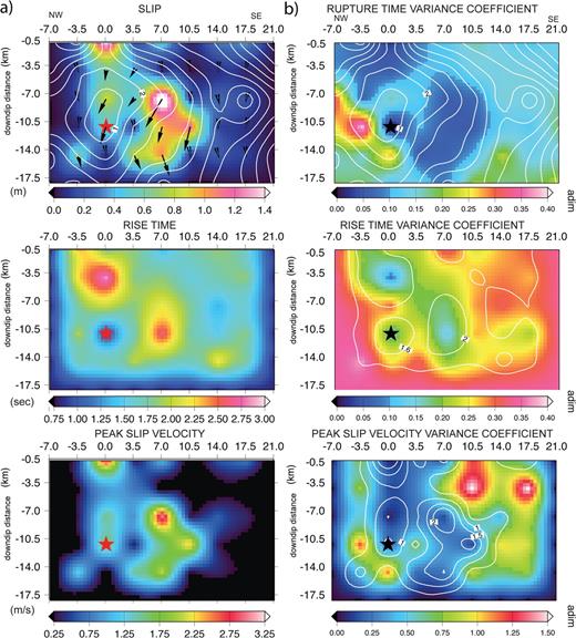
(a) Inverted rupture model (average model from ensemble inference) of the 2009 L'Aquila earthquake. Upper, middle and bottom panels show total slip, rise time and peak slip velocity distributions, respectively. The rupture time is shown by contour lines in white colour at 1 s intervals; the black arrows displayed in top panel represent the slip vector; (b) coefficient of variation (CV). Top, middle and bottom panels display the rupture times, the rise time and the peak slip velocity spatial distributions of the CV, respectively. White contour lines in each panel display the spatial distribution of the associated model parameter.

Open in new tabDownload slide

Figure 8

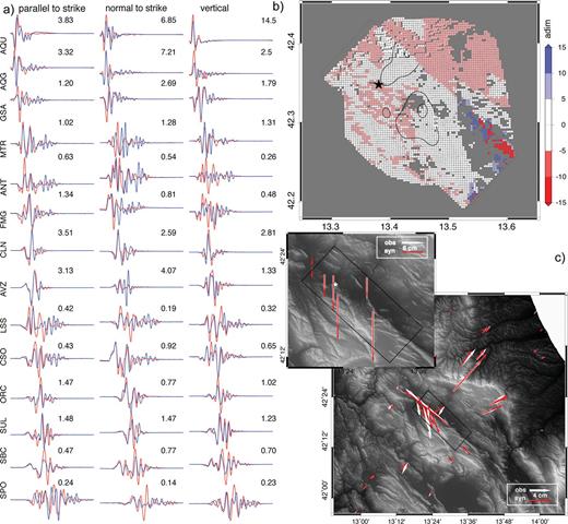
(a) Comparison of recorded strong motion (blue lines) with synthetic waveforms computed from the inverted rupture model displayed in Fig. 7 (red lines). Numbers with each trace are peak amplitude of the observed waveforms in cm s⁻¹. (b) Relative error between the observed and synthetic DInSAR displacement; black lines show slip contouring. (c) Comparison of measured (white arrows) with synthetic (red arrows) horizontal (main panel) and vertical (inset panel) coseismic displacement.

Open in new tabDownload slide

The misfits resulting from the average model shown in Fig. 7(a) are listed in Table 2, together with the cost function values associated with the best-fitting model (not shown in this study). The joint inversion yields cost function values very similar to those obtained by inverting the single data sets, and a better fit to DInSAR data than the strong motion model, confirming that this model contains the key source features of the rupture process. Moreover, for the joint inversion the cost function values of the average source model and those of the best-fitting models are quite similar, again confirming that selection of model parameters performed by our inversion approach is robust.

The analysis of the coefficient of variation is useful to image the dispersion of the three model parameters around their respective average values displayed in the average kinematic model. We have not shown the standard deviation because this parameter is meaningless, as discussed by Monelli & Mai (2008). These authors discussed the deviation of the model parameters from a Gaussian distribution, which limits the statistical interpretation of the standard deviation. The distributions of the coefficient of variation for rupture times, rise time and peak slip velocity shown in Fig. 7(b) reveal a small dispersion of model parameters in the fault portions that slipped during the L'Aquila earthquake. This suggests that the average model contains stable features of the rupture history and allows the identification of the relevant properties. In particular, we emphasize that in the shallow portion of the fault located updip the rupture nucleation, the coefficient of variation indicates a small dispersion, while on the shallow southeast part of the fault, where imaged slip amplitudes are very small, the coefficient of variation is large suggesting that the resolution available with the used data set is limited.

To discuss the inferred source model, Fig. 9 shows the comparison between the slip distribution resulting from the joint inversion (bottom panel) and those inferred by inverting each independent data set. This comparison confirms that the joint inversion yields a rupture model containing all the key features of the previously discussed models. The joint inversion better constrains the location and the extension of the deeper slip patch located southeastwards from the hypocentre along the strike direction, in agreement with DInSAR and GPS observations. In particular, the joint inversion displays a less extended slip patch at shallow depth updip from the hypocentre with respect to the GPS and strong motion solutions, although the inferred peak slip amplitudes are still larger than those suggested by DInSAR inversion. Moreover, the joint inversion confirms that the surface breakages observed on the Paganica Fault are associated with the deep and large slip concentration. Finally, the joint inversion model displays almost no slip on the shallowest southeast border of the fault plane, where afterslip has been located (Cheloni et al. 2010), consistently with DInSAR observations. The rupture time distribution of this model is slightly smoother than that retrieved by solely inverting strong motion data, although the rupture propagation still shows remarkable heterogeneities and a peculiar rupture history.

Figure 9

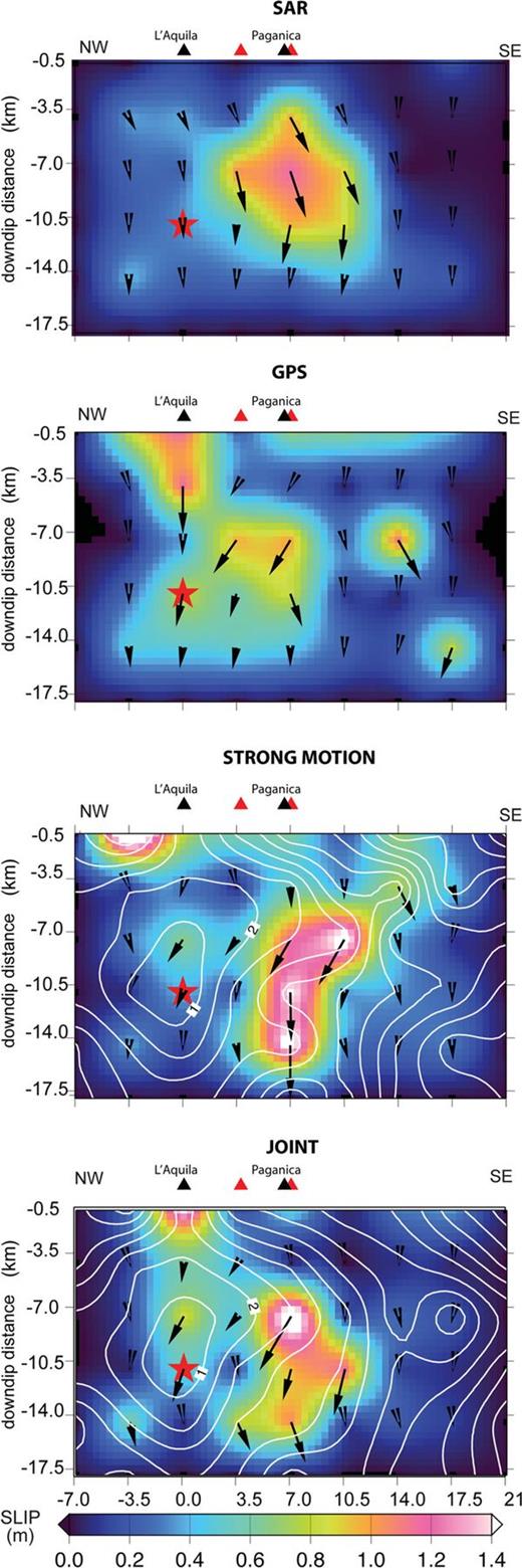
Slip maps from the inversion of the real data. From top to bottom are displayed the slip distributions for the DInSAR, GPS, strong motion and joint inversion of the three data sets. In each panel, black and red triangles show the location of the L'Aquila city and Paganica village, and the observed surface breakages, respectively.

Open in new tabDownload slide

7 Discussions

The main outcome emerging from our modelling is the evident and somewhat surprising complexity of the rupture process, in particular considering its moderate magnitude and the small dimension of the fault area. The source complexity is characterized by: (i) the heterogeneous distribution of model parameters on the fault plane, (ii) the variability of the rupture velocity and (iii) the peculiar spatial evolution of the rupture front. To further discuss these features, we have plotted in Fig. 10 several snapshots of the slip velocity on the fault plane imaged every 0.5 s. The white and red stars indicate the main shock hypocentre and the location of the IP phase, respectively; the contour lines in each panel display the areas of the highest slip concentrations: white line shows the area that slipped more that 0.65 m and the yellow contour line the area that slipped more than 1.2 m.

Figure 10

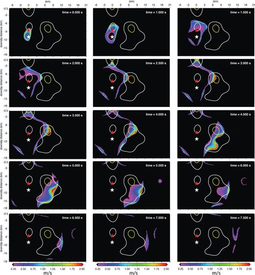
Time snapshots of slip velocity in m s⁻¹ on the fault plane, imaged every 0.5 s. White and yellow lines show the regions of the fault plane that slipped more than 0.65 m and 1.2 m, respectively. White and red stars display the location of the hypocentre and the impulsive phase (IP), respectively.

Open in new tabDownload slide

This figure clearly shows that the rupture began to propagate updip for nearly 1.5–2.0 s, with almost no along-strike propagation during this time window. Moreover, the first concentration of slip is located nearly 2 km updip from the hypocentre and occurs between 0.5 and 1 s. This is consistent with the location and timing of the IP phase (Michelini et al. 2009; Di Stefano et al. 2011). The inverted model is characterized by an initial updip rupture propagation (lasting nearly 2 s) associated with a relatively high rupture velocity (∽3.5–4.0 km s⁻¹). After nearly 2 s, the rupture starts to propagate along the strike direction and at depths shallower than the nucleation. The main slip patch begins to break after nearly 2.5 s, while the slip concentration at nucleation depths breaks after nearly 4.0–4.5 s with a clear delay with respect to the initial updip propagation. The rupture is stopped along the shallower SE corner of the fault plane. In this fault region the lack of coseismic slip is likely compensated by afterslip cumulated on the assumed fault plane during several weeks following the main shock (Cheloni et al. 2010) or alternatively by post-seismic deformation distributed on a complex pre-existing fault pattern (Valoroso et al. 2011). The rupture front propagation and the spatial evolution of slip velocity are quite peculiar; the rupture of the deeper slip patch looks similar to an asperity breakage (Spudich & Cranswick 1984; Spudich & Beroza 1988) and it is associated to spatial variations of the rupture velocity.

To better discuss these features we have plotted in Fig. 11(a) both the local rupture velocity imaged from rupture times and the rupture velocity vector as defined in eq. (4). This figure clearly points out the initial updip propagation at nearly 4 km s⁻¹. This rupture velocity is not super-shear, because S-wave speed in that volume is as large as 4.2 km s⁻¹. The relatively high rupture velocity located at depth, just below the largest slip patch, is lower than the rupture speed in the fault portion updip of the hypocentre (vector length scales with amplitude). Moreover, the initial speed of the rupture front (within the first second) ranges between 2.0 and 3.7 km s⁻¹, which excludes a slow rupture between the EP and IP phases.

Figure 11

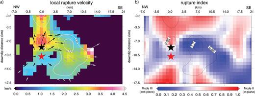
(a) Local rupture velocity distribution on the fault plane for the 2009 L'Aquila main shock overlapped by the slip contour (white line, in metres) and by the rupture velocity vectors (black and grey arrows show the rupture velocity vector for rupture times between 0 and 2.0 s and over 2.0 s, respectively). (b) Rupture index displaying the rupture mode across the fault plane for the 2009 L'Aquila earthquake. Values towards 1 correspond to a pure Mode II (inplane) rupture, values towards 0 to a pure Mode III (antiplane) rupture. Values in between correspond to a mixed rupture mode.

Open in new tabDownload slide

Furthermore, we have computed the rupture mode coefficient proposed by Pulido & Dalguer (2009) and defined as

(7)

which allows the imaging of the rupture mode on the fault plane.

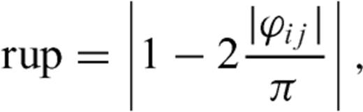
Fig. 11(b) displays the distribution on the fault plane of the rupture mode coefficient. According to Pulido & Dalguer (2009), rup = 0 corresponds to a Mode II crack propagation, while rup = 1 to a Mode III. As expected from Fig. 11(a), the updip initial propagation is characterized by a Mode II and the along-strike rupture propagation by a Mode III. The high (subshear) rupture velocity characterizing the updip propagation is consistent with a Mode II crack propagating in a medium with relatively high S-wave speed.

Di Stefano et al. (2011) have imaged the P-wave velocity and the Poisson ratio anomalies in the crustal volume containing the fault plane by inverting aftershocks traveltimes. These authors concluded that a relatively low Poisson ratio characterizes the crust around the main shock hypocentre, while larger values of Poisson ratio are found in correspondence of both the high slip patch and the large rupture velocity at depth. We emphasize that the zone of transition between enhanced and low Poisson ratio values coincides with the fault area where the along-strike rupture propagation has been initially impeded and delayed. This might reveal the presence of a structural control of rupture history, which did not allow the immediate rupture propagation along the strike direction. The easiest interpretation of this feature involves the role of heterogeneity of material properties, which might result in heterogeneous rheological properties. However, the foreshock pattern (Chiaraluce et al. 2011b) suggests the presence of a complex fault system at depth near the nucleation area, which might imply the presence of a geometrical barrier.

8 Conclusions

In this study we have inverted GPS, DInSAR data and strong motion waveforms to image the coseismic slip and the rupture history during the 2009 April 6 M_w 6.1 L'Aquila main shock. The separate inversion of each independent data set allows us to image the coseismic slip distribution on the fault plane. The comparison between these inverted models sheds light on the complexity of the rupture process emphasizing the presence of two main slip patches as well as a heterogeneous rupture time distribution. Furthermore, the joint inversion of GPS, DInSAR and strong motion data allows the identification of the relevant features of the rupture history and better constrains the position and the spatial extension of the slip patches on the main shock fault plane.

The rupture model proposed in this study corroborates seismological observations, which suggest an initial stage of the rupture characterized by a first slip concentration located updip the nucleation and rupturing between 0.5 and 1.0 s (see Fig. 10). It is worth noting the agreement between the location of the IP phase (Michelini et al. 2009; Di Stefano et al. 2011) and the position of the first slip concentration (see the red star location in Fig. 10).

The rupture history is characterized by two distinct phases: the first phase comprises the initial updip rupture propagation and a strong rupture acceleration associated with a modest seismic moment release (∽25 per cent of the total), followed by a second phase (which began ∽2.5 s after the rupture initiation, see Fig. 10) characterized by the along-strike rupture propagation and the failure of the deep slip patch (∽75 per cent of the total seismic moment). Therefore, despite our rupture model confirms previous findings that pointed out the evident along-strike directivity (Pino & Di Luccio 2009; Akinci et al. 2010, among several others), it also reveals an initial updip directivity that lasted for nearly 2 s and likely affected the ground motion waveforms in the L'Aquila area. The updip and along-strike rupture propagations are separated in time and associated with two distinct rupture modes: Mode II and Mode III, respectively. Therefore, for the L'Aquila earthquake Mode II and Mode III are nearly decoupled, in high slip patches.

Our inversion results show that the observed Paganica surface breakages (EMERGEO WG 2010; Cinti et al. 2011) are associated with the deep slip patch. No relevant surface ruptures were observed above the shallow slip patch located updip the hypocentre. Moreover, inverted models predict the absence of coseismic slip on the shallower southeastward corner of the fault plane, where Cheloni et al. (2010) found evidences of post-seismic slip (afterslip) lasting several weeks after the main shock. The amplitude of the afterslip observed in this fault portion, during the first month following the main shock, is comparable to the retrieved coseismic surface breakage. These results suggest complex slip partitioning within the near-surface crustal layer that likely affected the geological observations.

Acknowledgments

We thank Lauro Chiaraluce, Stefano Pucci, Alberto Michelini, Salvatore Stramondo, Nicola D'Agostino, Daniele Cheloni, Simone Atzori, Raffaele Di Stefano, Laura Scognamiglio and Claudio Chiarabba for helpful discussions and for sharing preliminary results of their investigations. We thank the Editor Eiichi Fukuyama, Martin Mai and an anonymous reviewer for their comments and criticisms, which allowed us to improve our manuscript. Antonella Cirella was supported by the NERA-EC (262330) project.

References