Laplace-domain waveform inversion versus refraction-traveltime tomography

Summary

Introduction

Accurate velocity analysis is an important factor to accurate subsurface imaging of oil and gas reservoirs. Although conventional semblance-based and traveltime tomographic analysis techniques are the most commonly used velocity analysis tools (Woodward et al. 2008), recent advances in full waveform inversion have generated considerable interest (Virieux & Operto 2009). A major advantage of full waveform inversion is that it is an automated rather than an interpreter-intensive technique. In addition, full waveform inversion more fully utilizes the amplitude and phase information content of seismic data, properly handling multipathing, caustics and other wavefield phenomena. Despite these advantages, full waveform inversion requires a well-defined starting model to produce an accurate result.

There has been considerable work devoted to constructing such a starting velocity model, with one workflow based on starting velocity models generated from reflection seismic data and a second workflow generated using refraction seismic data. Sirgue et al. (2009) and Plessix et al. (2010) have found that pre-stack-migration-driven velocity models provide a good starting model. In contrast, crustal seismologists use lower-fold but longer-offset data amenable to refraction tomography, which serve as their starting model for full waveform inversion (Brenders et al. 2008). Laplace-domain waveform inversion has also been suggested as a technique to construct a good starting model (Shin & Cha 2008). Various studies of the Laplace-domain waveform inversion have been followed by several geophysicists (Shin & Ha 2008; Bae et al. 2010; Chung et al. 2010; Ha et al. 2010; Shin et al. 2010; Pyun et al. 2011).

The Laplace-domain wavefield is obtained by multiplying the seismic signal by an exponentially decaying function, exp(−αt), where α is the Laplace constant, and taking the zero-frequency component of its Fourier transform (Shin & Cha 2008). Although the mathematics and numerical implementation is similar to multifrequency full waveform inversion, Laplace-domain waveform inversion uses a suite of J (f_j = 0+iα_j) frequencies, providing a long-wavelength starting model at a fraction of the cost, and with minimal investment in new software development and maintenance. Although both refraction-traveltime tomography and Laplace-domain waveform inversion produce smooth velocity models amenable to subsequent full waveform inversion or migration, the velocity resolution of the two techniques is significantly different.

Refraction-traveltime tomography is routinely used to estimate the thickness and velocity of the shallow weathering zone. This weathering zone model is then used to compute static corrections needed to remove the distortions of reflection events due to the heterogeneous weathering zone. Refraction-traveltime tomography commonly uses a ray tracing method to compute the first-arrival traveltimes and their Fréchet derivatives. Many geophysicists favour ray-based refraction-traveltime tomography because of its simplicity and efficiency, giving rise to a library of such methods (Hampson & Russell 1984; Schneider & Kuo 1985; White 1989; Zhu & McMechan 1989; Docherty 1992; Qin . 1993; Cai & Qin 1994; Stefani 1995; Shtivelman 1996; Zhang & Toksoz 1998). Because classical ray theory does not easily handle diffractions, ray-based tomography is limited to relatively smooth velocity models. For this reason, ray-based methods provide limited information about the subsurface (Wu & Toksoz 1987; Woodward 1992; Zelt & Barton 1998). Finite-frequency refraction-traveltime tomography (Luo & Schuster 1991; Dahlen et al. 2000; Hung et al. 2000; Pyun et al. 2005; Min & Shin 2006; Ellefsen 2009) overcomes some of these limitations. In particular, Pyun et al. (2005) developed a first-arrival traveltime tomography algorithm using damped monochromatic wave equation, which mimics the finite-frequency traveltime tomography using single frequency component only.

In this study, we adopted the approach of Pyun et al. (2005) as a representation of refraction-traveltime tomography because their algorithm is similar to Laplace-domain waveform inversion that it can represent simple and multiple diffractions. Although the objective of Laplace-domain waveform inversion is the same as first-arrival traveltime tomography, and although the Pyun et al.'s (2005) approach is mathematically similar to Laplace-domain waveform inversion, there are significant differences between the two methods. The objective of this paper is to compare and contrast Laplace-domain waveform inversion and traveltime tomography through a suite of tutorial examples. We begin our discussion by reviewing the theoretical basis of two techniques. Next, we compare forward-modelled first-arrivals computed over two simple salt block models exhibiting sharp corners and a high velocity contrast. We continue this comparison through a suite of increasingly complex forward models. Finally, we perform the first-arrival traveltime tomography using damped monochromatic wavefields and Laplace-domain waveform inversion using a suite of synthetic models generated using wave equation finite-difference algorithms.

Laplace-Domain Waveform Inversion

The discretized finite-element formula of the Laplace-domain wave equation can be expressed as (Shin & Cha 2008)

(1)

where S is a complex matrix composed of the stiffness matrix, K, and mass matrix, M,

(2)

where α is a real Laplace constant (or damping factor) and and are the Laplace-domain wavefield and source vectors, respectively. We can express the Laplace-domain wavefield as

(3)

where u (x, t) is the time-domain wavefield and ω_r is the real angular frequency. We note that this Laplace-domain wavefield is equivalent to the zero-frequency component of the damped wavefield in the time domain (Shin & Cha 2008).

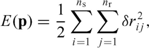
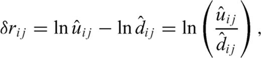
The implementation of a Laplace-domain waveform inversion algorithm is nearly the same as that of a conventional frequency-domain full waveform inversion. When we implement the Laplace-domain waveform inversion, however, we adopt Shin & Min's (2006) logarithmic misfit function because the wavefields in the Laplace domain are too small to be measured by the conventional l2 misfit function.

Our Laplace-domain waveform inversion uses the back-propagation algorithm of Pratt et al. (1998) to calculate the gradient direction efficiently. The logarithmic objective function for Laplace-domain waveform inversion is defined as

(4)

(5)

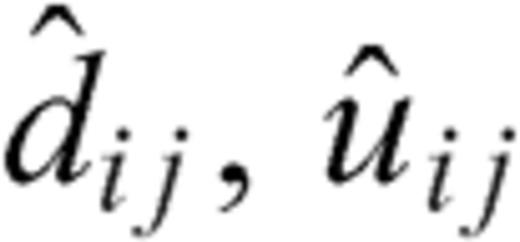
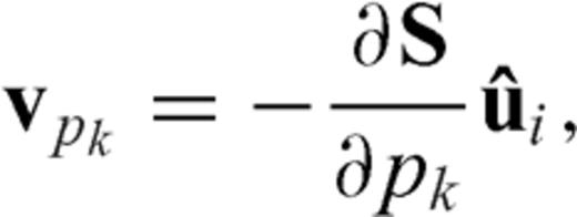
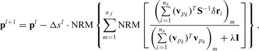
where p is a model parameter vector, and are the observed wavefield, the modelled wavefield and their residual in the Laplace domain at the jth receiver for the ith source, respectively; the values n_s and n_r are the total numbers of shots and receivers. Using the back-propagation algorithm, we can calculate the gradient direction of the objective function as follows:

(6)

where

(7)

and k is the model parameter index, the superscript T denotes the matrix transposition and v_Pkis the virtual-source vector.

We update the velocity model on the basis of the gradient method and the pseudo-Hessian matrix (Shin et al. 2001). Specifically, we follow the method of Ha et al. (2009) to update the velocity model,

(8)

where n_f is the total number of Laplace constants, λ is the damping term used to stabilize the pseudo-Hessian matrix, I is the identity matrix, Δs is the step-length, m is the index for the Laplace constant, NRM indicates the normalizing operation and the superscript l denotes the iteration number. We iteratively update the model parameters until the data misfit becomes sufficiently small.

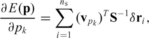
First-Arrival Traveltime Tomography

A wave equation implementation of first-arrival traveltime tomography shares many features with the Laplace-domain waveform inversion, such as the need for the computation of Fréchet derivatives, a normal equation, local minima problem and non-uniqueness of a general inverse problem (Pratt et al. 1998; Pyun et al. 2005). In particular, the first-arrival traveltime tomography technique developed by Pyun et al. (2005) is strongly related to Laplace-domain waveform inversion owing to the utilization of the damped wavefields. Unlike ray-based methods, both of these methods accurately represent first-arrival wave path (or a bundle of ray paths). For this reason, we decided to compare the first-arrival traveltime tomography algorithm described by Pyun et al. (2005) to Laplace-domain waveform inversion.

We use the damped wavefield method suggested by Shin et al. (2003) to calculate the first-arrival traveltime. The frequency-domain wavefield can be expressed as

(9)

where ω = ω_r + iα is the complex angular frequency. We assume that a time signal can be approximated by a series of weighted spikes and all events following the first arrival can be suppressed by using a large damping factor, as was done by Shin et al. (2003). Then, the damped frequency-domain wavefield can be expressed as

(10)

and

(11)

where A(x) is the amplitude and τ(x) is the traveltime from a source point to a receiver or an image point. By taking the logarithm of both sides of eq. (11), we obtain

(12)

and

(13)

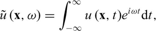
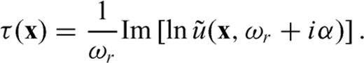
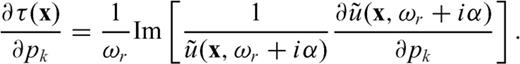
Using the eq. (13), the first-arrival traveltime can be calculated by isolating the imaginary part of the logarithm of the frequency-domain wavefield and dividing it by the real angular frequency. In particular, when we calculate the first-arrival traveltime, it is important to use a suitable value of complex angular frequency. We addressed the way of selecting proper complex angular frequency in the next chapter (eqs 16 and 17). We can extract the traveltime residual by subtracting the modelled traveltime from the traveltime picked from the seismic data measurements.

To carry out the first-arrival traveltime tomography and analyse the sensitivity patterns, we calculate the Fréchet derivative by differentiating eq. (12) with respect to model parameter p_k and dividing it by the original wavefield. The result of this operation is

(14)

From eq. (14), the Fréchet derivative of the first-arrival traveltime can be extracted as

(15)

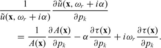
We adopt the conventional l2 misfit function, unlike Laplace-domain waveform inversion, which utilizes the logarithmic misfit function. We next follow the steepest descent method to update the velocity model according to the procedure of Pyun et al. (2005).

Comparison of Damped Wavefields

Although both methods reviewed in the previous sections use the damped wavefield, there are theoretical differences between them. In the case of first-arrival traveltime tomography, we fit the phase of the first-arrival events at a very low real frequency and sufficiently high imaginary frequency (or damping factor). To avoid the phase wrapping phenomenon, we choose a sufficiently low angular frequency (Min & Shin 2006) given by

(16)

where t_max is the maximum recording time, which is chosen to be the maximum possible traveltime in a given velocity model. To generate the damped wavefield necessary for the calculation of first-arrival traveltimes, it is quite important to select a suitable damping factor. However, there is no proven analytical equation to select the damping factor (Ellefsen 2009). Instead, the empirical relationship was extracted from the dispersion curves (Shin . 2003):

(17)

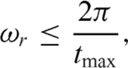
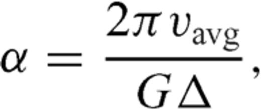
where v_avg is the average velocity, G is the number of gridpoints per wavelength and is the grid spacing. Shin . (2003) proposed the optimal number of gridpoints per wavelength as 15 by numerical tests. In this paper, we also select the optimal value of the damping factor by this empirical relationship (Shin . 2003).

In the case of Laplace-domain waveform inversion, on the other hand, we do not match the phase but the amplitude of the damped wavefield. Because we set the real angular frequency to zero, the Laplace-domain wavefield has no phase term. Accordingly, the Laplace-domain waveform inversion uses only the amplitude component of the damped wavefield. The amplitude of the first-arrival signal is dominant in the Laplace-domain wavefield when we use a large Laplace constant, whereas the amplitudes of later-arriving signals play a role when we use a small Laplace constant. Ironically, the first-arrival traveltimes are closely related to the Laplace-domain wavefields even though the traveltimes came from phase information and the Laplace-domain wavefields came from amplitudes. We attribute this irony to the exponential damping kernel of the Laplace transform by which we may encode (forward Laplace transform) phase information into amplitude although it is difficult to decode (inverse Laplace transform) it.

We demonstrated the above properties of damped wavefields using the simple seismograms shown in Fig. 1. Fig. 1(a) shows a common shot gather generated from a two-layered model. There are direct, refracted and reflected waves in the seismogram. Here, we neglected the other signals, such as multiples, for the sake of convenience. For comparison, we picked the first-arrival traveltime and muted all of the signals following the first-arrival event, as shown in Fig. 1(b). We calculated the logarithmic amplitude and phase of the damped wavefields for first-arrival traveltime tomography (Fig. 2). The phases perfectly simulate the first-arrival traveltimes for both seismograms (Fig. 2b). Interestingly, the amplitudes qualitatively resemble the phases even though we did not use the amplitudes for inversion. Fig. 3 displays the logarithmic amplitudes and phases of the damped wavefields used for the Laplace-domain waveform inversion when the Laplace constants are α= 1 and α= 10, respectively. The damped wavefields for the Laplace-domain waveform inversion have only an amplitude, unlike those for first-arrival traveltime tomography. Note that there are significant amplitude difference between the signal containing only the first arrivals and that containing the later arrivals as well. This difference increases with smaller values of the Laplace constant, α. Thus, by choosing an appropriately small value of α, Laplace-domain waveform inversion is sensitive to first and later arrivals, whereas the first-arrival traveltime tomography with a large value of α is sensitive only to the first arrivals.

1

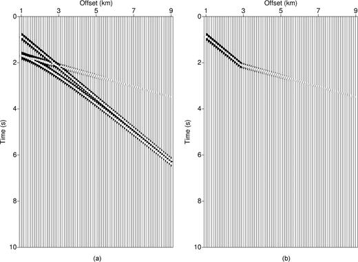
Sample seismograms: Panel (a) shot gather including direct, refracted and reflected events; Panel (b) shot gather only including first-arrival events.

Open in new tabDownload slide

2

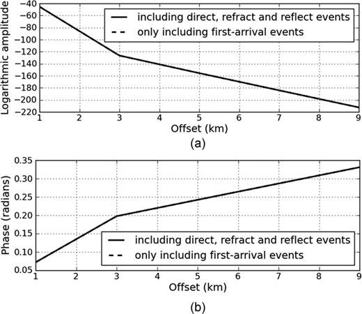
Panel (a) logarithmic amplitude and Panel (b) phase of damped wavefield for traveltime tomography.

Open in new tabDownload slide

3

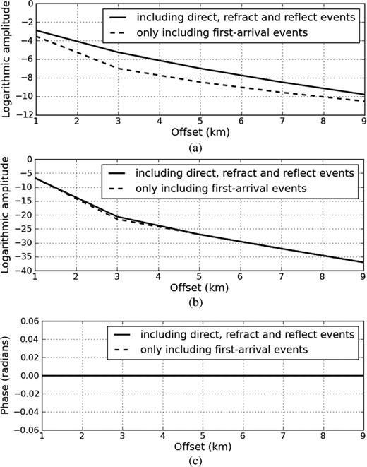
Logarithmic amplitude when Laplace constants are (a) 1 and (b) 10 and (c) phase of damped wavefield for Laplace-domain waveform inversion.

Open in new tabDownload slide

Laplace-domain waveform inversion is sensitive to amplitude damping (and thereby suppressing the influence) of later-arrivals, with the amount of damping being proportional to exp(—αt). Unfortunately, exp(—αt) amplifies noise before the first-arrival which negatively impacts the inversion results (Ha et al. 2010). For this reason, a great care should be taken to mute the noise before the first-arrrivals before the Laplace-transform of seismograms. First-arrival traveltime tomography, however, does not remove noise before first-arrival signals, requiring only the picking of first-arrival events. Such muting is common practice in seismic migration and adds little to the complete velocity analysis through pre-stack depth migration workflow.

Surface Responses

To illustrate the differences between Laplace-domain waveform inversion and first-arrival traveltime tomography, we compared the surface responses of two methods for the simple blocky models shown in Fig. 4. We assumed that the dimensions of the blocks in Fig. 4 were 1000 × 600 m and that their velocity was 4.5 km s⁻¹. The background velocity was assumed to be 1.5 km s⁻¹. The two models differ in that the high-velocity blocks are located at 1.8 and 0.6 km, respectively. We used a 2-D finite-element method to simulate the wave propagation. We simulated one shot on the surface at a horizontal distance of 4 km. The first derivative of a Gaussian function was chosen as the source wavelet. The traveltimes and wavefields were measured by 750 receivers with an interval of 20 m. To generate the traveltimes for the first-arrival traveltime tomography, we selected a frequency of 0.1 Hz to avoid the phase-wrapping phenomenon. We chose α= 18.85 as the damping factor using eq. (17).

4

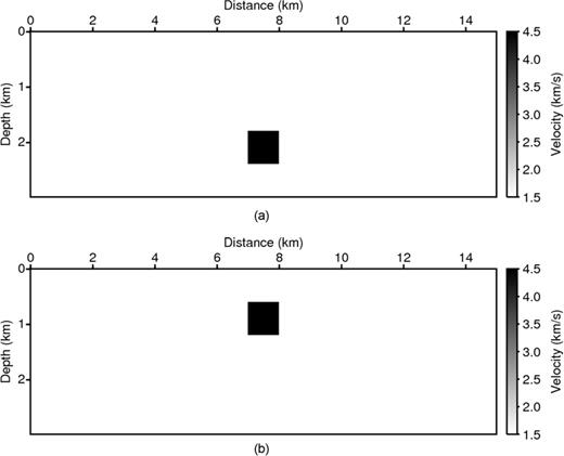
Simple homogeneous models (v = 1.5 km s⁻¹) containing a (a) deep and (b) shallow constant 4.5 km s⁻¹ velocity inclusion.

Open in new tabDownload slide

Fig. 5(a) shows the first-arrival traveltimes for a homogeneous model (dotted line) and the model containing a deep high-velocity block (solid line) and a shallow block (dashed line). As expected, the traveltime curve for the homogeneous model shows a single linear moveout event corresponding to the direct arrival. The deep block is identical to that of the homogeneous model. The refracted waves generated for this model arrive later than the direct wave for all offsets displayed. In contrast, the traveltime curve for the model with a shallow block shows the direct arrival at near offsets and the refracted event at far offsets. Fig. 5(b) shows the traveltime differences between the homogeneous model and the two models containing a high-velocity block. We note that the refracted wave is detectable only in the model containing the shallow block.

5

Panel (a) modelled first-arrival traveltimes corresponding to the two models shown in Fig. 4 for a source on the surface at 4 km. Note that the deep block is not represented by the first arrivals for the range of modelled receivers. Panel (b) shows the difference in measured traveltimes picks between the homogeneous and block models.

Open in new tabDownload slide

Fig. 6(a) shows the corresponding Laplace-domain wavefields on the surface. To simulate the Laplace-transformed wavefields, we adopted a 2-D finite-element modelling scheme in the Laplace domain as Shin & Cha (2008) did. For the Laplace-domain waveform inversion, we selected Laplace constants of α= 1 and α= 10. The black curves show the Laplace-domain wavefields for the homogeneous model (dotted line) and for the models containing the deep high-velocity block (solid line) and the shallow block (dashed line) when the Laplace constant, α= 1. The grey curves show the same comparison for a Laplace constant of α= 10. To make the Laplace-domain wavefields discernable, we displayed those wavefields on a logarithmic scale (Figs 6b and c). The Laplace-domain waveform inversion was carried out by normalizing the gradient direction with respect to each Laplace constant and adding the scaled gradient directions. Accordingly, the relative difference is more meaningful than the absolute one. For smaller values of the Laplace constant (Fig. 6b), both the shallow and deep block models give rise to anomalous events. On the other hand, when the Laplace constant is large (Fig. 6c), only the model with the shallow block gives rise to a large anomaly, similar to the result from the first-arrival refraction model.

6

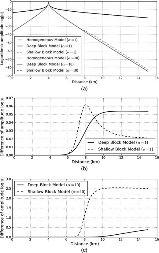
Panel (a) Modelled events measured along the surface using the Laplace-domain formulation and homogeneous (dotted), deep block (solid) and shallow block models (dashed). Panels (b) and (c) show the differences between shallow and deep block models from the homogeneous model for Laplace constants of 1 and 10, respectively.

Open in new tabDownload slide

Sensitivity Analysis

The sensitivity, or Jacobian, matrix is a measure of the change in response data with respect to a given model parameter. Measurements that are more sensitive to given model parameters will generally resolve them better. In this section, we analyse the sensitivity of both first-arrival traveltimes and Laplace-domain wavefields for three models: a homogeneous model, a linearly increasing velocity model and a five-layer model. We calculate the sensitivity kernels for offset distances of 3.12 km (short offset) and 13.54 km (long offset). We use a 2-D finite-element modelling technique to calculate the traveltimes and Laplace-domain wavefields. To calculate the first-arrival traveltimes, we set the real angular frequency to 0.1 Hz and chose the damping factor computed from eq. (17).

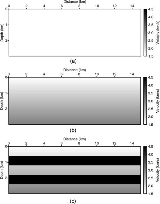
The homogeneous velocity (v = 1.5 km s⁻¹) model is 15 km wide and 3 km deep (Fig. 7a). Because the first-arrival event of the homogeneous model consists only of the direct wave travelling along the surface, such a model is considered to be a poor starting model for ray-based tomography. Figs 8(a) and (b) display the normalized sensitivity kernels calculated by eq. (15). The sensitivities are non-zero only near the surface because the first–arrival events do not penetrate deeply into the homogeneous model, which indicates that the first-arrival traveltime tomography can invert the velocity only at the surface.

7

Models used to evaluate algorithm accuracy: Panel (a) constant-velocity model, Panel (b) model with linearly increasing velocity with depth and Panel (c) five-layer model.

Open in new tabDownload slide

8

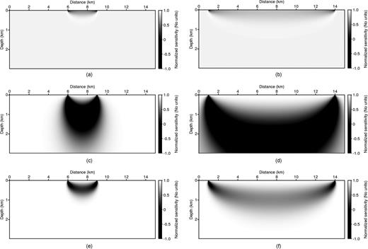
The normalized sensitivity kernels generated from (Panels a, b) traveltime tomography and from Laplace-domain waveform inversion when the Laplace constants were (Panels c, d) 1 and (Panels e, f) 10. The left column displays the short offset distance (3.12 km) conditions, and the right column shows the long offset distance (13.54 km) environment. The model is the constant-velocity model shown in Fig. 7(a).

Open in new tabDownload slide

Figs 8(c)–(f) show the normalized sensitivity kernels associated with the Laplace-domain waveform inversion when the Laplace constants are α= 1 and α= 10. When the Laplace constant is large, the sensitivity pattern is similar to that of the first-arrival traveltime tomography and is sensitive only to shallow velocity perturbations. When the Laplace constant is small, however, the algorithm is sensitive to the velocity in deeper areas. This means that the sensitivity of the Laplace-domain waveform inversion depends on the Laplace constant, α. In addition, we can infer that the Laplace-domain waveform inversion using a homogeneous model may work well, unlike the traveltime tomography.

Fig. 7(b) shows the linearly increasing velocity model where the velocity ranges from 1.5 to 3.0 km s⁻¹ with depth. In practice, such a linearly increasing velocity model is commonly used as a starting model for both the first-arrival traveltime tomography and the Laplace-domain waveform inversion techniques. Figs 9(a) and (b) show the normalized sensitivity kernels for first-arrival traveltime tomography. We easily note that this sensitivity shape is different from the previous one (Figs 8a and b) calculated from the homogeneous model. The shape mimics that of a diving or turning wave. When the source-receiver offset distance is long, the wave paths reach to greater depths, unlike those in the homoneneous model. The penetration depth is still shallow when the offset distance is short. Figs 9(c)–(f) show the normalized sensitivity kernels used in the Laplace-domain waveform inversion for Laplace constants of α= 1 and α= 10. If the Laplace constant is high, the sensitivity kernel is similar to that obtained from the first-arrival traveltime tomography algorithm, although the wave paths are not distorted at the bottom. When the Laplace constant is low, the wave paths are broad and penetrate deeply even though the source-receiver offset distance is short. These images show that the Laplace-domain waveform inversion is more sensitive to localized velocity heterogeneities than those of first-arrival traveltime tomography, which lie farther outside the ray paths traversed in the linearly increasing velocity model with increasing depth.

9

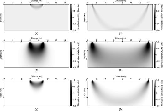
The normalized sensitivity kernels generated from (Panels a, b) traveltime tomography and from Laplace-domain waveform inversion when the Laplace constants were (Panels c, d) 1 and (Panels e, f) 10. The left column displays the short offset distance (3.12 km) conditions, and the right column shows the long offset distance (13.54 km) environment. The model is the linearly increasing velocity model in Fig. 7(b).

Open in new tabDownload slide

We next consider the more difficult example shown in Fig. 7(c), where conventional ray tracing would give rise to a shadow zone or ‘invisible’ layers. The velocities of the layers are 1.5, 4.5, 2.5, 4.5 and 3.0 km s⁻¹ from top to bottom. Figs 10(a) and (b) show the sensitivity kernels of the first-arrival traveltimes measured at near and far source-receiver offsets. It should be noted that whereas this algorithm is sensitive to perturbations in the upper two layers, it is insensitive to layers below the shallow high-velocity layer. These limitations are commonly observed in ray-based traveltime tomography. Fig. 11 shows the first-arrival traveltime generated from ray tracing in the five-layer model (Fig. 7c). The source is located at a horizontal distance of 1 km. No arrivals from deeper layers are measured along the surface of the model.

10

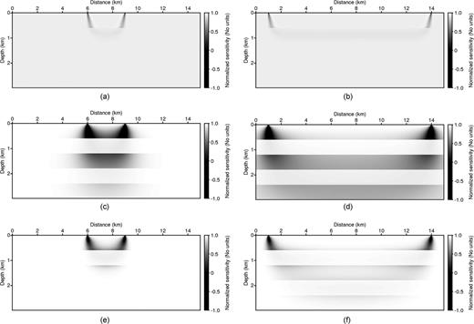
The normalized sensitivity kernels generated from (Panels a, b) traveltime tomography and from Laplace-domain waveform inversion when the Laplace constants were (Panels c, d) 1 and (Panels e, f) 10. The left column displays the short offset distance (3.12 km) conditions, and the right column shows the long offset distance (13.54 km) environment. The model is the five-layer model in Fig. 7(c).

Open in new tabDownload slide

11

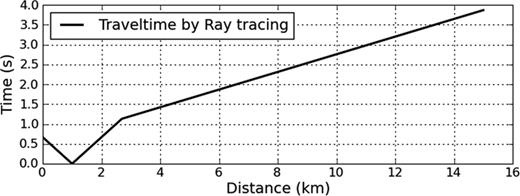
The first-arrival traveltime generated by the ray tracing method in the five-layer model displayed in Fig. 7(c). The source is located at a horizontal distance of 1 km. Only the direct arrival and refractions from the second layer are modelled. Deeper layers are not illuminated.

Open in new tabDownload slide

In contrast, Figs 10(c)–(f) display the normalized sensitivity kernels at near- and far-source-receiver offsets for the Laplace-domain waveform inversion when the Laplace constants are α= 1 and α= 10. The Jacobian matrices (and therefore solution sensitivities) are significantly different from those of first-arrival traveltime tomography. Even with a high Laplace constant, the solution is able to tunnel through the high-velocity overburden and be sensitive to the deeper low-velocity layer (such as slower clastics underlying faster carbonates or volcanics). Lower values of the Laplace constant, α, provide deeper sensitivity. Even for short source-receiver offset distances, the wave paths tunnel through, demonstrating that the Laplace-domain waveform inversion is sensitive to the low-velocity zone below the high-velocity layer and can potentially invert the high-velocity structures at greater depths.

To increase the penetration depth, first-arrival traveltime tomography requires a long-offset distance. In reality, there are limitations imposed by exploration equipment and the environment. The Laplace-domain waveform inversion technique, however, can be implemented by using a low Laplace constant properly as well as by increasing the offset distance.

Inversion Examples

From the analysis of the Jacobian kernels using a suite of simple models, we predict that the Laplace-domain waveform inversion will provide more robust solutions than first-arrival traveltime tomography. The first numerical model we used was the five-layer model shown in Fig. 7(c). The dimensions of the model are 15 × 3 km, with a grid spacing of 20 m. For the numerical examples, we modelled 188 sources with an interval of 80 m at a depth of 20 m. We used the first derivative of a Gaussian function as the source wavelet. We measured the pressure data at 751 receivers located at a depth of 20 m. Fig. 12(a) shows the starting velocity model, which is a linearly increasing velocity model with velocities ranging from 1.5 km s⁻¹ at the top to 3.0 km s⁻¹ at the bottom.

12

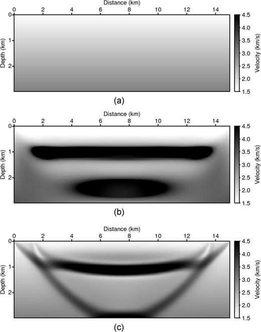
Inversion results for the five-layer model using all surface sources and receivers: Panel (a) the initial model and inverted results using Panel (b) Laplace-domain waveform inversion and Panel (c) refraction-traveltime tomography. The Laplace-domain inversion is quite close to the true model, except for the areas that are not illuminated by the acquisition aperture. Refraction tomography gives an acceptable but less accurate (bowed) result in the second layer and artefacts associated with edges of illumination limits at deeper levels.

Open in new tabDownload slide

Fig. 12(b) shows the velocity model inverted by the Laplace-domain waveform inversion at the 1000th iteration. Twenty Laplace constants ranging from α= 1 to α= 20 with an interval of δα= 1 were simultaneously used for the inversion. It should be noted that not only the upper high-velocity layer was correctly recovered but also the underlying low-velocity layer. Moreover, the partial illumination of the deeper high-velocity layer (layer four) was partially recovered. Fig. 12(c) shows the results obtained by the first-arrival traveltime tomography at the 200th iteration. In this example, we set the real angular frequency to f= 0.1 Hz and chose a damping factor of α= 40.21. From the results of the sensitivity kernels for the five-layer model (Figs 10a and b), we observed that the upper high-velocity zone (layer two) is more sensitive than the underlying layers. As a result, we can infer that both the top and bottom interfaces of the upper high-velocity layer (layer two) were clearly restored. Although the upper high-velocity zone was well recovered, deeper parts of the model were not correctly recovered because the sensitivity kernel with the first-arrival traveltime tomography does not provide a complete illumination of the target as shown in Fig. 9(b). In case of the first-arrival traveltime tomography, the deeper high-velocity layer was not detected at all.

In another example, we compared the difference between first-arrival traveltime tomography and Laplace-domain waveform inversion using the synthetic BP model (Billette & Brandsberg-Dahl 2005) shown in Fig. 13(a). The BP model was 67 km long and 12 km deep. Fig. 13(b) shows synthetic wavefields in the Laplace domain when the Laplace constants are α= 1, 5, 10 and 20. Those wavefields were obtained using a 2-D finite-element Laplace-domain modelling scheme (Shin & Cha 2008). Fig. 13(c) displays the synthetic traveltime generated by the damped wavefield method (Shin . 2003) at a horizontal distance of 35 km in the BP model.

13

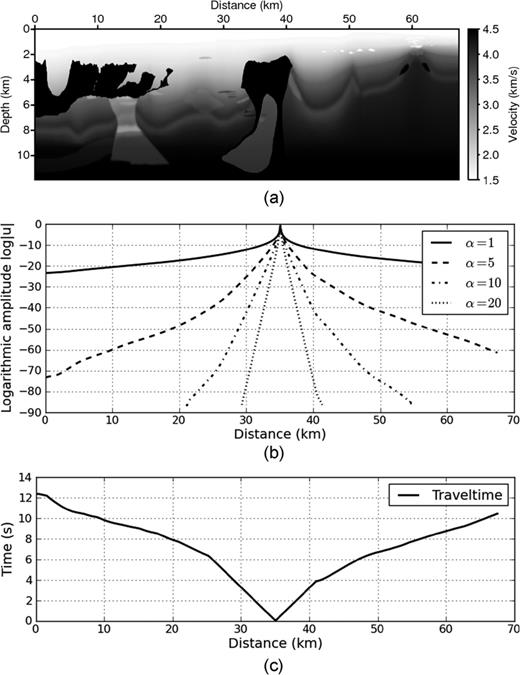
The synthetic BP model: Panel (a) the true model, Panel (b) Laplace-domain wavefields and Panel (c) traveltime measured at a horizontal distance of 35 km.

Open in new tabDownload slide

In this test, we carried out the first-arrival traveltime tomography using a smoothing regularization (by smoothing the gradient direction at each iteration) for more fair comparison between two methods. Laplace-domain waveform inversion does not require any regularization effort, unlike first-arrival traveltime tomography. Because Laplace-domain waveform inversion fits the low-wavenumber feature of seismograms, it naturally smoothes the solution. On the other hand, first-arrival traveltime tomography needs regularization.

Fig. 14(a) shows the starting linearly increasing velocity model ranging from 1.5 to 4.1 km s⁻¹. Fig. 14(b) is the velocity model inverted from the Laplace-domain waveform inversion at the 500th iteration, and Fig. 14(c) is that from the first-arrival traveltime tomography at the 100th iteration. For the Laplace-domain waveform inversion, we simultaneously used the same twenty Laplace constants as those in the previous five-layer example. For the first-arrival traveltime tomography, we also used a real angular frequency of f= 0.1 Hz and α= 17.89 as the damping factor. From the Laplace-domain waveform inversion results (Fig. 14b), we can observe that the three upper salt structures are well imaged. However, the models inverted by first-arrival traveltime tomography (Fig. 14c) are recovered only at the shallow structures, and the quality of these images is not satisfactory.

14

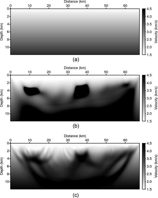
The inversion examples from the refraction-traveltime tomography and the Laplace-domain waveform inversion: Panel (a) the linearly increasing starting model, Panel (b) themodel inverted by the Laplace-domain waveform inversion and Panel (c) the model inverted by the refraction-traveltime tomography.

Open in new tabDownload slide

To investigate the dependency of the Laplace-domain waveform inversion technique on the starting velocity model, we performed the inversion again using the homogeneous starting velocity model shown in Fig. 15(a). The velocity model inverted by Laplace-domain waveform inversion is shown in Fig. 15(b). We hypothesize that the inverted images generated from the Laplace-domain waveform inversion are relatively insensitive to the starting velocity model. In contrast, we could not obtain a velocity model by first-arrival traveltime tomography when using the homogeneous model as a starting velocity model (Fig. 15a) because there were no refracted waves in the homogeneous media.

15

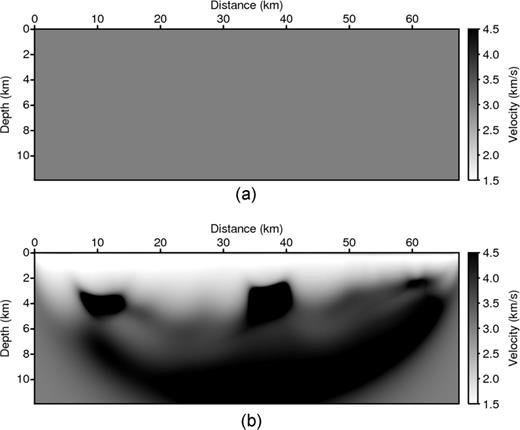
The inversion examples from the refraction-traveltime tomography and the Laplace-domain waveform inversion: Panel (a) the entire homogeneous starting model and Panel (b) the model inverted by the Laplace-domain waveform inversion. We could not obtain the velocity model inverted by the refraction-traveltime tomography because there were no refracted waves in the homogeneous media.

Open in new tabDownload slide

Conclusions

Classic refraction tomography use explicit ray tracing that may or may not honour diffracted first arrivals. To better compare first-arrival refraction-traveltime tomography to the Laplace-domain waveform inversion algorithm, we used a first-arrival traveltime tomography algorithm based on damped monochromatic wavefields that accurately represents first-arrival wave path. Other than muting noise before the first arrival, Laplace-domain waveform inversion does not require picking. By weighting the measured seismic trace by a suite of damping functions, exp(—αt), the amplitudes of later-arrivals contribute to final velocity model, but does not require determining which event corresponds to a given ray family. The contribution of these later-arrivals results in increased sensitivity to deeper velocity anomalies and decreased sensitivity to the accuracy of the starting velocity model.

The sensitivity patterns clearly describe the relationship between the Laplace-domain waveform inversion and the first-arrival traveltime tomography. Large values of the Laplace constant, α, heavily weights the first arrivals and provides a sensitivity pattern similar to that of first-arrival refraction-traveltime tomography. Smaller values of the Laplace constant, α, increase the contribution of later arrivals, and are more sensitive to deeper velocity anomalies. By combining inversions for a suite (e.g. 20, in this paper) of Laplace parameters, α, we obtain a robust solution that balances both shallow and deeper events.

The computation time of frequency-domain refraction-traveltime tomography is significantly higher than that of classic ray tracing based first-arrival refraction-traveltime tomography. The cost of the Laplace-domain waveform inversion is 20 times higher than frequency-domain refraction-traveltime tomography if we use 20 values of α. However, computation cost is typically small compared to algorithm development and maintenance costs. Ray-based algorithms (such as Kirchhoff migration and classical tomography) are significantly more difficult to write and maintain than wave equation, grid-based algorithms (such as reverse-time migration and Laplace-domain wavefield inversion). Furthermore, the kernel of both the frequency-domain refraction-traveltime tomography and Laplace-domain waveform inversion algorithms is nearly identical to that of the desired target application—(multi) frequency-domain wavefield inversion. In this manner, algorithmic improvements in frequency-domain wavefield inversion translate directly into improvements in Laplace-domain waveform inversion to generate the needed starting model. We, therefore, envision Laplace-transform based inversion as a pre-processing module in a larger, more complete wavefield inversion package.

Acknowledgments

The authors would like to thank TOTAL for their financial support and Sukjoon Pyun's work was supported by INHA UNIVERSITY Research Grant.

References