An efficient and flexible approach to the calculation of three-dimensional full-wave Fréchet kernels for seismic tomography—II. Numerical results

Summary

1 Introduction

While finite-frequency effects have been considered almost ever since the beginning of digital seismology, seismic tomography still heavily relies on either asymptotic ray theory for body-wave traveltimes at the high-frequency end (e.g. Dziewonski et al. 1977; Inoue et al. 1990; Grand 1994; Su et al. 1994; Van der Hilst et al. 1997; Bijwaard & Spakman 2000) or a hybrid of surface-wave modal and ray approach at the long-period end (e.g. Woodhouse & Dziewonski 1984; Zhang & Tanimoto 1993; Panning & Romanowicz 2006; Lebedev & van der Hilst 2008). Apart from a few intensely monitored areas such as southern California, Japan and Taiwan, uneven and poor path coverage in seismic tomography often puts strong demand on a priori and other constraints to regularize the inversions. The combination of approximate wavefield modelling, insufficient path coverage and regularization, strongly degrades the resolution of tomographic models. As a result, whereas the images obtained from regional and global seismic tomography are robust on the relatively large-scale structures of the Earth, tomographic images are still fuzzy and unreliable for structures at subcontinental or smaller scales. Using accurate sensitivity kernels calculated by normal-mode summation, regional surface wave tomography using data from dense broad-band arrays can indeed resolve structures as small as 100 km, smaller than the size of the first Fresnel zone (Chevrot & Zhao 2007). However, the application of the normal-mode approach has been so far rather limited owing to a relatively low numerical efficiency.

Finite-frequency tomography takes into account the finite and limited bandwidth nature of seismic waves and models waveforms more accurately so that physically more realistic structural sensitivities of the data can be incorporated in the inversion. By a rigorous treatment of waveform perturbation in standard seismic tomography problem, 2-D Fréchet or sensitivity kernels of waveforms to wave speed were first obtained (Luo & Schuster 1991; Woodward 1992; Yomogida 1992; Li & Tanimoto 1993). Developments in the past dozen years provided theory and algorithms for calculating 3-D Fréchet kernels for finite-frequency seismic observations based on 1-D (Marquering et al. 1999; Dahlen et al. 2000; Hung et al. 2000; Zhao et al. 2000; Zhou et al. 2004; Nissen-Meyer et al. 2007) or 3-D (Tromp et al. 2005; Zhao et al. 2005) models.

One of the challenges in 3-D finite-frequency tomography is the heavy computational labour required in the calculations of 3-D kernels. Dahlen et al. (2000) and Hung et al. (2000) introduced an efficient algorithm based on paraxial ray approximation which made it practical to use 3-D finite-frequency kernels in global tomography (Montelli et al. 2004). Zhou et al. (2004) extended this approach to surface waves. However, ray theory approximation is only applicable to high-frequency waves in the far-field, and can not be used to describe non-geometrical arrivals such as diffracted phases. In addition, the near-field contribution also has an important effect on traveltime tomography (Favier et al. 2004), especially for structures near sources and receivers.

In the previous paper (Zhao & Chevrot 2011, hereafter referred to as Paper I), we have introduced the definition of strain Green's tensors (SGTs), and shown that the displacement field due to an earthquake is simply the inner product of the third-order single-side strain Green's tensor (SSGT) and the moment tensor of the earthquake source. Moreover, a quantity called the waveform perturbation density representing the contribution of a local model perturbation to waveform anomaly can be expressed in terms of the convolution of the SSGT from the receiver to the perturbation location and a fourth-order two-side strain Green's tensor (TSGT) from the source to the perturbation location. The merit of TSGT and SSGT is such that they can be pre-calculated for a chosen reference earth model and organized into a SGT database, so that they can be quickly retrieved rather than calculated in all subsequent calculations for synthetics or Fréchet kernels. Furthermore, by exploring the symmetry properties of the moment tensor and the elasticity tensor, only 10 elements of the 21-element third-order SSGT and 20 elements of the 81-element fourth-order TSGT are necessary in the SGT database for all possible Fréchet kernel calculations. In principle, the SSGT and TSGT can be calculated using any wave simulation methods, from the approximate but numerically efficient ray asymptotic approach for geometrical arrivals (e.g. Dahlen et al. 2000; Hung et al. 2000), the exact but more elaborate normal-mode (Zhao et al. 2000; Zhao & Jordan 2006), direct-solution (e.g. Cummins et al. 1994a,b; Geller & Takeuchi 1995; Kawai et al. 2006), GEMINI (Friederich & Dalkolmo 1995) and 2-D spectral-element (Nissen-Meyer et al. 2007) methods for 1-D earth models, to the purely numerical finite-difference (Zhao et al. 2005; Chen et al. 2007) and spectral-element (Tromp et al. 2005; Tape et al. 2009) methods for fully 3-D reference models implemented in parallel computing environment.

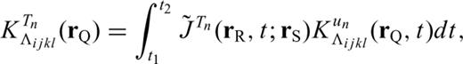
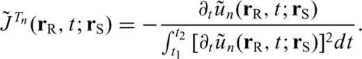
The wavefield modelling method we choose in the current study is the normal-mode summation. The theoretical background of the SGTs and the calculation and establishment of the SGT database by normal-mode summation has been described in Paper I. In this paper, we discuss the application of the SGT database in calculating Fréchet kernels for finite-frequency seismic tomography. We first present the expression for the waveform Fréchet kernel in terms of the SGTs, which is then used to obtain the Fréchet kernels of various other seismic observables, such as traveltime, amplitude and SKS-splitting intensity (Chevrot 2000), for isotropic and anisotropic model parameters. We also present numerical examples of Fréchet kernels for a variety of surface and body waves.

2 Synthetics and FrÉchet Kernels Expressed in Terms of SGTS

By virtue of the representation theorem (e.g. Aki & Richards 2002), once the Green's tensors for a particular earth model are available, seismic displacement at any arbitrary location from any given source can be obtained. Using the SGT, the displacement field generated by an earthquake of moment tensor M located at r_S can be expressed as

1

where h (r, t; r_S) is the so-called SSGT defined in Paper I. It is a third-order tensor whose element h_ijk(r, t; r_S) represents the (j, k)-component of the strain field at r_S due to a unit impulsive point force acting at r in ith coordinate direction. For convenience the moment tensor M in eq. (1) is assumed to have a Dirac-delta function δ (t) time history. For a moment tensor with a different time history, the displacement can be obtained by simply convolving the time function in M with eq. (1). In this paper, the Einstein summation rule is assumed unless otherwise stated. In regional and global seismological problems, a convenient coordinate system is composed of three basis vectors along vertical (Z), radial (R) and transverse (T) directions. Therefore, indices i, j and n in eq. (1) designate any one of these components in this coordinate system.

Seismic tomography consists of finding the 3-D earth model perturbations that minimize the waveform misfit , which quantifies the difference between the recorded waveform u (r_R, t; r_S) and the synthetic waveform predicted by the reference model. Here, we use a tilde to indicate quantities in the reference model. An important quantity in deriving the Fréchet derivatives of seismic observables is the waveform perturbation density, which is linearly related to the model perturbations

2

where H_lkpq(r_Q, t; r_S) are elements of the fourth-order TSGT defined in Paper I. The geometry of the source, receiver and perturbation locations are depicted in Fig. 1. An element H_lkpq(r_Q, t; r_S) represents the (l, k)-component of the strain field at r_Q due to a unit force couple at r_S with its force and arm along q and p axes, respectively. Therefore, H (r_Q, t; r_S): M represents the strain field at r_Q generated by an earthquake at r_S with moment tensor M. In both Paper I and here, we have omitted the tilde on the SGTs h and H, however it is understood that they are always evaluated in the reference model.

Figure 1

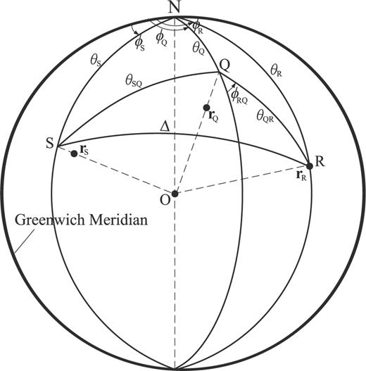
Geometry of the source at r_S, receiver at r_R and an arbitrary location r_Q at which the Fréchet kernel is being calculated. S, R and Q are the surface projections of r_S, r_R and r_Q, respectively. Here r_R and R coincide since the receiver is assumed to be on the surface.

Open in new tabDownload slide

The quantity δ U_n(r_Q, t) in eq. (2) provides the contribution to the n-component waveform perturbation due to a local perturbation per unit volume in the fourth-order elasticity tensor , hence the name waveform perturbation density. From the expression in eq. (2), we can obtain the Fréchet derivative of the waveform recorded at location r_R and time t with respect to a given element of the elasticity tensor at r_Q

3

which represents the sensitivity of the waveform to Λ_ijkl(r_Q). This partial derivative is also referred to as the Fréchet kernel of the n-component waveform for model parameter Λ_ijkl(r_Q).

2.1 Fréchet kernels for isotropic perturbations of the elasticity tensor

Expressions of the waveform Fréchet kernels for isotropic model parameters have been derived in Paper I, where we have also shown that traveltime Fréchet kernels can be expressed as

4

where the integral is over the time window [t₁, t₂] that contains the seismic signal of interest, and

5

As described in Paper I, eq. (5) is obtained for the delay time δ T_n defined as the lag time of the maximum in the cross-correlagram between synthetic and record u_n(r_R, t; r_S). The measurement of the amplitude anomaly can be defined through waveform cross-correlation as

6

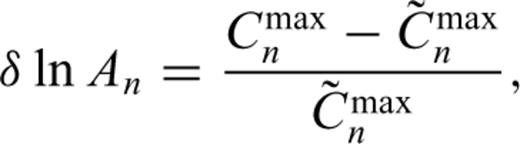
where C^max_n and are the maximum amplitudes in the synthetic-record cross-correlagram C_n(t) and the synthetic–synthetic auto-correlagram , respectively. In other words, C^max_n= C_n(δ T_n), and . Using the definitions of cross- and autocorrelations, we can show that under the Born approximation

7

with

8

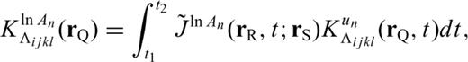
In fact, for any arbitrary measurement d obtained through certain linear operations of the waveforms, we can always define a functional dependent upon the reference model such that the Fréchet derivative of the observable with respect to Λ_ijkl takes on the general form

9

This relation gives us a linear relationship between the seismic observable d and the perturbations of Earth's elastic parameters, from which we can formulate a tomographic inverse problem

10

In this study, we are only concerned with the perturbation in the elastic parameters. Perturbations in other model parameters such as density, seismic discontinuity topography and attenuation, specified by the bulk and shear quality factors, can be considered in a similar way (Dahlen 2005; Dahlen & Zhou 2006; Zhou 2009). This, in principle, enables us to invert seismic observations for every elastic and anelastic parameters in the earth model. In practice, however, only a very limited number of elements in the elasticity tensor can be reliably recovered by seismological means. These parameters include the isotropic compressional and shear wave speeds and a few specifically defined anisotropy parameters.

2.2 Fréchet kernels for anisotropic perturbations of the elasticity tensor

Statistical analysis of olivine and pyroxene aggregates, a good analogue of upper-mantle material, has shown that, to first order, upper mantle is weakly anisotropic and can be well-approximated by hexagonal symmetry (Becker et al. 2006). This result is important because it allows us to simplify considerably the description of upper-mantle anisotropy. Assuming hexagonal symmetry, the elasticity tensor can be expressed in terms of seven parameters (Chevrot 2006)

11

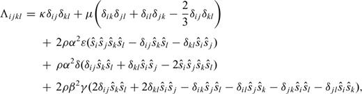
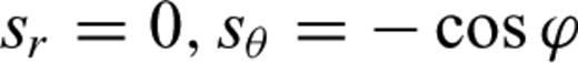
where κ and μ are the isotropic bulk and shear moduli, respectively, and α and β are the associated isotropic P- and S-wave speeds, respectively. The quantities ɛ, δ and γ are three dimensionless anisotropic parameters, and is a unit vector specifying the orientation of the symmetry axis. Anisotropic parameters ɛ and γ quantify P- and S-wave anisotropy, respectively, while δ is an additional parameter describing the shape of the slowness surfaces for P and S waves. The symbols δ_ij with subscripts are the Kronecker delta.

Given the orientation of the symmetry axies , the Fréchet kernels for the anisotropic parameters ɛ, δ and γ can be derived by substituting eq. (11) into eq. (2), and we have

12

13

14

More explicit expressions of the above Fréchet kernels are given in the Appendix for radial anisotropy (transversely isotropic or hexagonal structure with a vertical axis of symmetry) and azimuthal anisotropy (horizontal axis of symmetry). Equivalent expressions were derived in Panning & Nolet (2008) under surface-wave formalism.

By perturbing the axis of symmetry in eq. (11), we can also derive the Fréchet kernels for its individual components

15

Eqs (12–15) are derived for a perturbation of the waveform. For other seismic observables, by substituting those equations into eq. (9), and using the proper functionals for the observable, we can obtain the expressions of their Fréchet kernels for the isotropic and anisotropic model parameters.

In constraining upper-mantle anisotropy from shear wave splitting observations, we cross-correlate the transverse-component SKS wave generated by anisotropy with its radial or longitudinal counterpart, and define the amplitude of the cross-correlagram at zero lag time as the SKS-splitting intensity (Chevrot 2000)

16

where δ u_T(r_R, t; r_S) is the perturbation in the transverse-component waveform, that is, transverse-component SKS generated by anisotropy from the originally purely radially-polarized SKS wave, and

17

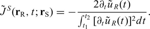
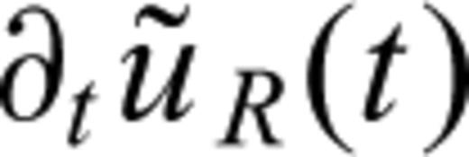In eq. (17), is the radial-component velocity seismogram of SKS wave in the reference model. Comparison between in eq. (17) with in eq. (10) in Paper I suggests that the SKS-splitting intensity is proportional to the delay time between fast and slow quasi-shear waves. From previous discussion, we can express the Fréchet kernels of SKS-splitting intensity for a given model parameter m as

18

with m being any one of the model parameters such as the elastic moduli or wave speeds, and the corresponding expressions for the waveform Fréchet derivatives are given in eqs (21–24) in Paper I and in eqs (12–15) here.

3 Numerical Examples of FrÉchet Kernels

In this section, we present numerical examples of Fréchet kernels of seismic observables commonly used in seismic tomography (traveltimes, amplitudes and SKS-splitting intensity). The expressions derived in the previous section for the Fréchet kernels in terms of SGTs are completely general and can be used for arbitrary earth models with lateral variations. In the present paper, we present results based on normal-mode theory, which provide exact Green's tensors for spherically symmetric models in which medium properties only vary with the radius. The calculation of SSGT and TSGT and the establishment of their databases have been discussed in Paper I, where examples of the SGTs for earth model PREM (Dziewonski & Anderson 1981) as well as synthetics obtained from them have been presented. The SGTs used in the kernel calculations here are computed by summing all the normal modes for model PREM up to 0.15 Hz (period of about 7 s), resulting in Green's tensor databases that are accurate up to about 0.12 Hz, or period down to about 8 s.

3.1 Fréchet kernels of geometrical arrivals

Body waves with turning points far away from discontinuities in the Earth exhibit simple ray-theory behaviour with traveltimes increasing linearly along the ray paths and amplitudes influenced by geometrical spreading and reflection and transmission coefficients at seismic discontinuities. Anelastic attenuation affects both the phase and amplitude of seismic waves through physical dispersion and intrinsic attenuation, respectively. In this study, we assume that the Earth is perfectly elastic, which means that the amplitudes of seismic waves are only affected by focusing and defocusing caused by seismic heterogeneities. Here, we present Fréchet kernels of both traveltimes and amplitudes for the perturbations of seismic wave speeds.

Fig. 2 displays the Fréchet kernels of the traveltime and amplitude of vertical-component P wave and transverse-component S wave. The traveltime kernels in Fig. 2 exhibit the classical banana–doughnut shape characteristic of kernels for geometrical arrivals (e.g. Dahlen et al. 2000). The sensitivity vanishes along the geometrical ray path, increases away from the ray path until reaching a maximum, decreases again to zero and then changes sign, defining the first and second Fresnel zones. Sensitivity is strongest near the source and the receiver owing to both the focusing of waves and near-field contributions. The kernels for P and S waves are computed in a similar frequency band, yet the S wave has clearly a narrower first Fresnel zone because the width of the first Fresnel zone is proportional to the square root of the wavelength. In contrast, the sensitivity of the amplitude is maximum along the geometrical ray path, and as a result the first Fresnel zones of amplitude kernels are thinner than their corresponding traveltime counterparts. Although the traveltime kernels are counter-intuitively zero along the ray paths, the values of both traveltime and amplitude kernels in the first Fresnel zones are all physically intuitive in that a wave-speed increase located in the first Fresnel zone results in negative traveltime and amplitude perturbations, that is, an advance in arrival time and a (defocusing-induced) decrease in amplitude, respectively.

Figure 2

Fréchet kernels of vertical-component P wave (top panels) and transverse-component SH wave (bottom panels) for P- and S-wave speeds α and β, respectively. The left panels are kernels of traveltimes and the right panels are kernels of amplitudes. Waves with period of 8 s or longer are included. Both the source and receiver are at the surface and the epicentral distance is Δ= 60°. Dashed lines indicate the Moho, the 410-km and the 660-km seismic discontinuities.

Open in new tabDownload slide

Fig. 3 shows the sensitivity kernels of traveltimes and amplitudes of transverse-component SS and ScS waves. The surface-reflected SS wave is a minimax phase, with a traveltime that is maximum within the source–receiver great-circle plane. In a realistic earth model with seismic discontinuities in the upper mantle and relatively high velocity gradient in the upper-mantle transition zone, many waves interfere with the SS arrival. Consequently, the sensitivity results from the superposition of the contributions of different arrivals (Zhao et al. 2000; Zhao & Chevrot 2003), which leads to a much more complicated pattern than the one for the direct arrivals shown in Fig. 2. In contrast, the ScS wave is a simple geometrical arrival with a clear banana–doughnut shaped traveltime kernel. The narrow strikes seen under the regular ScS sensitivity pattern are caused by waves arriving at a time close to the ScS phase that are included in the time window used for the calculation of the ScS kernels (see also discussion in Zhao et al. 2000). Randomly distributed oscillatory patterns occur occasionally, as a result of spatial or temporal aliasing, especially near the source and receiver. However, because of their rapidly spatially oscillating character and their smaller amplitude, they make little contribution to the spatial integral in eq. (10), and therefore these aliasing patterns would result in a negligible perturbation to traveltime and amplitude in any realistic earth model.

Figure 3

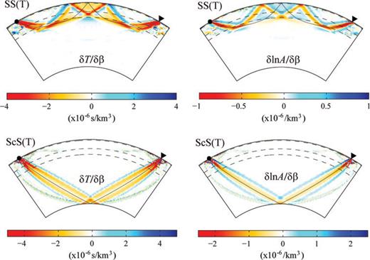
Fréchet kernels of transverse-component SS(H) wave (top panels) and ScS(H) wave (bottom panels) for S-wave speed β. The left panels are kernels of traveltimes and the right panels are kernels of amplitudes. Waves with period of 8 s or longer are included. Both the source and receiver are at the surface and the epicentral distance is Δ= 60°.

Open in new tabDownload slide

3.2 Fréchet kernels of surface waves

Normal-mode theory allows us to model exactly the propagation of all seismic waves in a spherically symmetric earth model. As a result, an important advantage of our normal-mode implementation in computing Fréchet kernels based on the SGT database is the capability to provide accurate results for non-geometrical arrivals such as surface waves.

Shown in Fig. 4 are the Fréchet kernels of Love-wave traveltime and amplitude for S-wave speed β at a depth of 21 km. The traveltime kernel of the Love wave has a relatively simple shape, with a more-or-less uniform first Fresnel zone and a fairly strong second Fresnel zone with opposite sign. The amplitude kernel consists of a rather narrow and weak first Fresnel zone but a relatively thick and strong second Fresnel zone. Furthermore, the Love-wave sensitivities in Fig. 4 display a slightly asymmetric pattern across the source–receiver great-circle path, resulting from the non-isotropic source radiation pattern.

Figure 4

Fréchet kernels of Love wave traveltime (left) and amplitude (right) for S-wave speed β at a depth of 21 km. Waves with period of 25 s or longer are included. The source is at a depth of 21 km with a focal mechanism shown by the beachball. The receiver is on the surface at an epicentral distance of Δ= 19°.

Open in new tabDownload slide

Love waves are only affected by the shear wave speed β. On the other hand, Rayleigh waves are influenced not only by the shear wave speed, but also by the P-wave speed α, especially at shallow depth (e.g. Dahlen & Tromp 1998; Bozdağ & Trampert 2008; Khan et al. 2009; Yang et al. 2010). The Fréchet kernels in Figs 5a and b illustrate respectively the vertical- and radial-component Rayleigh wave sensitivities to both P- and S-wave speeds. Although there are some differences in details, the sensitivity patterns of Rayleigh waves on different components are similar. For both vertical- and radial-component Rayleigh waves, the influences of P- and S-wave speeds on traveltime and amplitude are also similar, although the influence of S-wave speed encompasses a greater depth range and is about four times as strong as that of P-wave speed. The overall patterns of Rayleigh-wave kernels largely resemble their counterparts for Love wave, and the source radiation pattern also has a strong imprint.

Open in new tabDownload slide

Open in new tabDownload slide

Figure 5

(a) Fréchet kernels of vertical-component Rayleigh wave traveltime (left panels) and amplitude (right panels) for P-wave speed α (top panels) and S-wave speed β (bottom panels) at a depth of 21 km. Waves with period of 25 s or longer are included. Also shown are cross-sections of the kernels within the source–receiver great-circle plane down to 150-km depth. In each cross-section plot, the dashed line indicates the Moho discontinuity. The source is at a depth of 21 km with a focal mechanism shown by the beachball. The receiver is on the surface at an epicentral distance of Δ= 19°. (b) Fréchet kernels of radial-component Rayleigh wave traveltime (left panels) and amplitude (right panels) for P-wave speed α (top panels) and S-wave speed β (bottom panels) at a depth of 21 km. Waves with period of 25 s or longer are included. The source is at a depth of 21 km with a focal mechanism shown by the beachball. The receiver is on the surface at an epicentral distance of Δ= 19°.

3.3 Fréchet kernels of core–mantle boundary diffracted waves P_diff and S_diff

Waves diffracted along the core–mantle boundary (CMB) such as P_diff and S_diff are important seismic signals since they carry crucial information on structures in the lowermost mantle. However, due to the difficulty in modelling diffracted waves by asymptotic ray theory, the use of CMB diffracted phases in seismic tomography studies has been rare and somewhat simplified (e.g. Kárason & van der Hilst 2001; Li et al. 2008). These non-geometrical arrivals, on the other hand, are perfectly well modelled by normal-mode theory, as shown by the traveltime kernels of transverse-component Sdiff wave in Zhao et al. (2000) and Zhao & Jordan (2006). The SGT database provides a more efficient approach to model these CMB diffracted phases. The sensitivities of traveltimes and amplitudes of P_diff and S_diff waves to P- and S-wave speeds are shown in Fig. 6. The traveltime kernels still show the characteristic banana–doughnut shape with a very weak sensitivity along the ray path. However, the patterns in the vicinity of the CMB are more complicated, with alternating weak and strong sensitivities in the shadow zone along the CMB. In addition, the kernels in Fig. 6 clearly demonstrate that both the traveltimes and amplitudes of P_diff and S_diff can be influenced by mantle structures almost 500 km above the CMB, outside the D” layer.

Figure 6

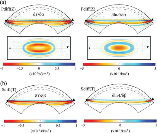
(a) Fréchet kernels of vertical-component P_diff wave in the source–receiver great-circle plane (top panels) and on the CMB for P-wave speed α. The left panels are kernels of traveltimes and the right panels are kernels of amplitudes. Waves with period of 8 s or longer are included. Both the source and receiver are at the surface and the epicentral distance is Δ= 105°. (b) Fréchet kernels of transverse-component S_diff wave for S-wave speed β. The left panels are kernels of traveltimes and the right panels are kernels of amplitudes. Waves with period of 8 s or longer are included. Both the source and receiver are at the surface and the epicentral distance is Δ= 105°.

Open in new tabDownload slide

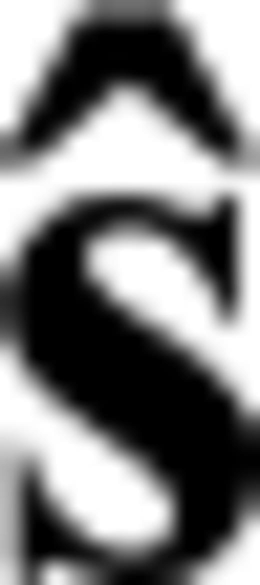
3.4 Fréchet kernels of SKS wave for anisotropic parameters

The sensitivities of the radial- and vertical-component SKS-wave traveltimes and amplitudes to the isotropic shear wave speed in the mantle are shown in Fig. 7. Even though the SKS wave follows a long path from the source to the receiver and undergoes S-to-P and P-to-S conversions at the CMB, the sensitivities of its traveltime and amplitude to shear wave speed still display the typical banana–doughnut pattern. Weak oscillations far away from the SKS ray path in the vertical-component kernels are due to contribution from P-wave energy. The signature of reflections at the free surface can also be seen in the radial-component kernels.

Figure 7

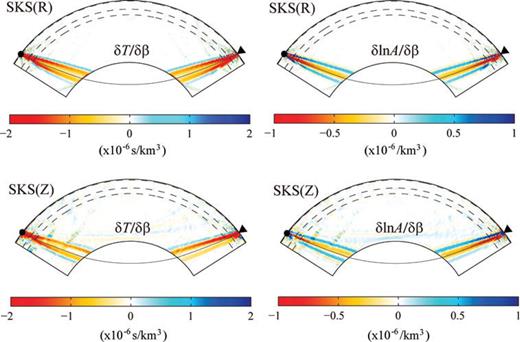
Fréchet kernels of radial- (top panels) and vertical-component (bottom panels) SKS wave for S-wave speed β. The left panels are kernels of traveltimes and the right panels are kernels of amplitudes. Waves with period of 8 s or longer are included. Both the source and receiver are at the surface and the epicentral distance is Δ= 105°. In this study, only sensitivities in the mantle are calculated. As a result, the sensitivities of the SKS wave to core structure below CMB are not shown.

Open in new tabDownload slide

Seismic anisotropy has a strong and complex influence on seismic waveforms. For example, anisotropy in the mantle ‘splits’ the radially-polarized SKS wave and generates a signal on the transverse component that would not be present should the Earth be isotropic and spherically symmetric. This property has been extensively used to investigate azimuthal anisotropy in the upper mantle. Traditionally, the SKS splitting has been modelled by vertically incoming plane SKS waves (Silver & Chan 1988, 1991). The influence of anisotropy on the splitting of finite-frequency SKS waves have recently been investigated (Favier & Chevrot 2003; Seminski et al. 2007, 2008), but their incorporation into a tomographic inversion scheme remains to be done.

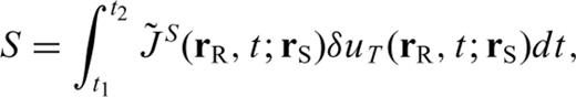
SKS-splitting intensity (Chevrot 2000), which measures the amplitude of transverse-component SKS wave with respect to its parent radial-component, is directly related to the anisotropic perturbations of the elasticity tensor (Favier and Chevrot 2003; Chevrot 2006). Another interesting property of this seismic observable is that to first-order it is not sensitive to isotropic perturbations of seismic velocities (Chevrot 2006), which makes it very suitable for imaging seismic anisotropy. The sensitivity of SKS-splitting intensity S to the isotropic shear wave speed β can be easily derived from eq. (18) with m =β. An example is shown in Fig. 8 along with the Fréchet kernels of the SKS-splitting intensity to perturbations in the hexagonal parameters ɛ and δ. The expressions for these kernels are provided in the Appendix (eqs A4 and A5). In the numerical examples in Fig. 8 and subsequent figures, the kernels for anisotropic model parameters are computed by assuming that the symmetry axis orientation is known. We should keep in mind, however, that the SGTs h and H are defined in the reference isotropic model, assumed to represent the isotropic average (κ and μ in eq. 11) of the anisotropic structure. The SGT databases are always calculated in an isotropic reference model, but they need not be recalculated if the isotropic average of the 3-D anisotropic model is sufficiently close to the average isotropic model. In practice, since upper-mantle anisotropy is small, we can always conduct the kernel computations using an isotropic reference model (here PREM).

Figure 8

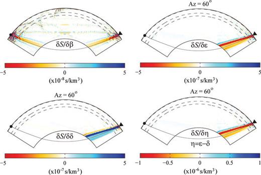
Fréchet kernels of SKS-splitting intensity S for the isotropic shear wave speed β and anisotropic parameters ɛ, δ and η=ɛ−δ in a model with a horizontal symmetry axis oriented in azimuth ϕ= 60°. When the axis of symmetry is either perpendicular (ϕ= 0°) or parallel (ϕ= 90°) to the propagation direction, no energy is scattered by either ɛ or δ into transverse-component and the corresponding ɛ and δ kernels vanish. Note that the sensitivity of SKS-splitting intensity to isotropic shear wave speed (top left) is much smaller than those to anisotropy parameters.

Open in new tabDownload slide

An observation from the kernels for ɛ and δ in Fig. 8 is that the contributions of ɛ and δ to splitting intensity have almost the same magnitude but are opposite in sign, which suggests to introduce a new anisotropic parameter η=ɛ−δ (Chevrot 2006). The sensitivity of the splitting intensity to the isotropic shear wave speed is apparently much smaller than that to anisotropy. For an anisotropic mantle, the sensitivity naturally arises in the second S-wave segment along the SKS path where transverse-component motion is generated from a purely radially polarized incoming SKS wave. Splitting intensity kernels are also characterized by zero sensitivity along the geometrical ray path, a result consistent with those of Favier & Chevrot (2003).

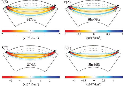
The sensitivity of the SKS-splitting intensity to the other anisotropy parameter γ is shown in Fig. 9 for three anisotropic models with horizontal axes of symmetry oriented with azimuths ϕ= 0°, 60° and 90° measured clockwise from north. The pattern is similar: the splitting intensity is insensitive to γ when the axis of symmetry is perpendicular or parallel to the propagation direction, whereas the sensitivity arises when ϕ= 60° after the SKS emerges from the CMB. Note that for a horizontal symmetry axis, the amplitude of γ kernels is an order of magnitude larger than those for ɛ,δ and η. Therefore, the best resolved parameter is likely γ in anisotropy imaging relying on splitting intensity measurements. In addition, the kernel for β are even smaller (Fig. 8), which implies that to first-order splitting intensity is insensitive to lateral variations in isotropic shear speed. This interesting property makes this seismic observable particularly well-suited for imaging upper-mantle anisotropy.

Figure 9

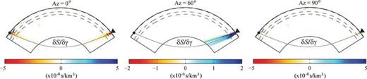
Fréchet kernels of SKS-splitting intensity S for anisotropic parameters γ in azimuthally anisotropic models with horizontal symmetry axes oriented in azimuths ϕ of 0° (perpendicular to propagation), 60° and 90° (parallel to propagation).

Open in new tabDownload slide

The kernels in Figs 8 and 9 can be used for imaging the strength of anisotropy if the orientation of the symmetry axis in the horizontal plane is known. To recover the orientation of the axis of symmetry, we need to compute the sensitivity kernels for the components of with the aid of eq. (15). To avoid the non-linearity introduced by trigonometric functions in and , Favier & Chevrot (2003) suggested to define an alternative set of two independent parameters γ_c=γ cos et al. 2ϕ and γ_s=γ sin et al. 2ϕ, which can be linearly related to the SKS-splitting intensity.

It is straightforward to derive the expressions for the sensitivities of SKS-splitting intensity to γ_c and γ_swith our SGT formalism. In a medium with a horizontal axis of symmetry of azimuth ϕ, the γ-related part of the elasticity tensor in eq. (11) can be written as

19

where the subscript //indicates a horizontal symmetry axis. Therefore, we obtain the following expressions of the waveform Fréchet kernels forγ_c and γ_s:

20

21

where we have omitted terms involving h_Trr since it is identically zero (see Eq. B11c in Paper I). By substituting eqs (20) and (21) into eq. (18), we can derive the Fréchet kernels of SKS-splitting intensity S for the new parameters γ_c and γ_s.

The sensitivities of the SKS-splitting intensity to γ_c and γ_s have been carefully examined in Favier & Chevrot (2003) assuming vertically incident plane SKS waves, and in Sieminski et al. (2007, 2008) using the full-wave spectral-element simulations. An important feature of the sensitivities of splitting intensity to γ_c and γ_sis their azimuthal variations in the forms of cos et al. (2ϕ_I) and sin et al. (2ϕ_I), where ϕ_I is the backazimuth of the incident SKS wave.

In Fig. 10, we display the SKS splitting intensity kernels for γ_c and γ_s for a suite of different backazimuths ϕ_I, where the cos et al. (2ϕ_I) and sin et al. (2ϕ_I)variations can be seen clearly. Such a dependence of the sensitivities on ϕ_I can also be seen in eqs (20) and (21). Substituting the expressions for h_Tθθ, h_Trθ, h_Trϕ and h_Tθϕ given in Eq. (B11c) in Paper I into eqs (20) and (21), we have

22

23

where the angle ϕ_RQ, as defined in Fig. 1, is effectively the backazimuth ϕ_I of the incident SKS wave. The fact that in Fig. 10 the kernel for γ_c is much smaller than that for γ_s when ϕ_I= 0° and ϕ_I= 90° implies that |h₈H_rrpqM_qp | are much larger than both |h₁₀H_rθpqM_qp | and |h₁₀H_rϕpqM_qp |. As a result, the sin et al. (2ϕ_RQ) and cos et al. (2ϕ_RQ) terms in eqs (22) and (23) both dominate the sin et al. ϕ_RQ and cos et al. ϕ_RQ terms, in good agreement with the observed sin et al. (2ϕ_RQ) and cos et al. (2ϕ_RQ) variations of the γ_c and γ_s kernels. This example clearly demonstrates that the SGT database approach allows us to efficiently compute accurate Fréchet kernels of the splitting intensities of finite-frequency SKS waves in a spherically symmetric earth model, opening new possibilities to imaging upper-mantle anisotropic structures with a fine spatial resolution.

Figure 10

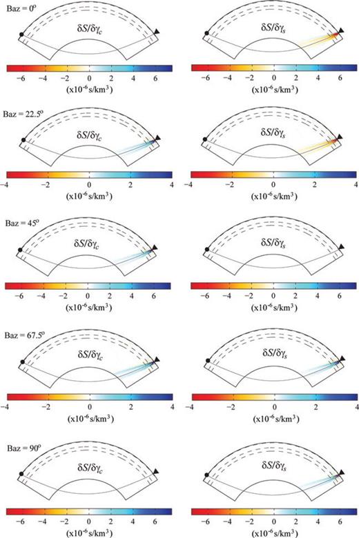
Fréchet kernels of SKS-splitting intensity S for anisotropic parameters γ_c (left columns) and γ_s (right columns) for SKS waves incident from backazimuths of 0°, 22.5°, 45°, 67.5° and 90°.

Open in new tabDownload slide

4 Discussion and Conclusions

We have developed a new approach for computing Fréchet kernels of seismic observables for any earth model parameter. In the SGT formulation, the sensitivity of waveform to the perturbation of any model parameter at r can be expressed in terms of the convolution between the third-order SSGT from the earthquake source to r and the fourth-order TSGT from r to the receiver. From the expression of waveform sensitivity it is straightforward to derive the Fréchet kernels of any seismic observable for all earth model parameters, including elastic and anelastic moduli, density and even the topographies of seismic discontinuities.

Under the SGT formulation, databases of SSGTs and TSGTs for a chosen reference model can be established to optimize the calculation of Fréchet kernels for seismic tomography. With the SGT databases, the calculation of Fréchet kernels is achieved by simple retrieval and convolution of appropriate SSGTs and TSGTs and there is no need for wavefield computations. This enables much more efficient calculations of Fréchet kernels for non-geometrical seismic signals that cannot be modelled by asymptotic ray theory.

We have also presented numerical examples obtained from a normal-mode implementation of this new approach for the Fréchet kernels of traveltimes and amplitudes of a variety of body and surface waves for P- and S-wave speeds and of the SKS-splitting intensity for hexagonal anisotropic parameters. The SGT database approach makes the normal-mode implementation much more realistic in conducting regional and global tomography using all seismic phases including surface waves and CMB diffracted P_diff and S_diff waves. The normal-mode approach also provides an efficient and convenient means to compute the Fréchet kernels of the SKS-splitting intensity for imaging upper-mantle anisotropic structure.

In computing a Fréchet kernel by the SGT approach, a significant portion of CPU time is spent on the retrieval of the SGTs for all the spatial sampling points at which the kernel is computed. As a result, the efficiency of the SGT approach is dependent on the number of spatial sampling points as well as the size and configuration of the SGT database. In our current straightforward implementation of the SGT approach, the SGTs are stored in the databases as fixed-length records with each record consisting of all the SGT elements, with each element being a 2400-point time-series, for a spatial gridpoint. Under this configuration, it takes about 30 min to compute a typical kernel with 24, 150 and 50 sampling points in the radial, source–receiver and transverse directions, respectively, using a 24-core Beowulf PC cluster. Although still a heavy computation, this performance represents a roughly 50 times increase in the speed of kernel calculation over the non-SGT normal-mode method for the frequency of interest up to 0.12 Hz or a period of ∼8 s (Chevrot & Zhao 2007). With this efficiency, it is practical to conduct full-wave finite-frequency tomography inversions using tens of thousands of data on a small cluster.

When the SGTs in the database are calculated in the time domain, the kernel calculations do not depend on the maximum frequency of the waves involved. Therefore, when the maximum frequency of interest increases, all one needs to do is to conduct the SGT calculation once for the new frequency band. In contrast, without using the SGT database the wavefield must be evaluated at each spatial sampling point. For most wavefield calculation methods, the computational labour increases drastically with the maximum frequency. For example, in normal-mode summation with consideration of coupling between each pair of modes, the computation increases as N², where N is the number of normal modes with eigenfrequencies below the maximum frequency (∼27 000 below 0.05 Hz and ∼100 000 below 0.1 Hz). For numerical methods such as the finite-difference and spectral-element methods, the number of spatial-temporal samples increases quarticly with the maximum frequency, resulting in dramatic increase in both memory and CPU time in numerical simulations.

It is also possible for specific tomography studies to establish targeted SGT databases to further improve the performance of the SGT approach. For instance, in a surface-wave tomography study we only need a database with SGTs at radial samples from the surface down to say 400 km depth instead of the whole mantle; whereas for anisotropic imaging using the SKS splitting intensity, we are mostly interested in teleseismic observations in the range of 85°–110° (Silver & Chan 1988), therefore a TSGT database with horizontal samples of 80°–115° and a SSGT database with horizontal samples of 0°–10° will be sufficient, and only radial samples in the upper mantle are necessary.

The size of SGT database can be reduced not only by limiting the number of spatial and temporal samples, but also by storing only the SGT elements needed for a specific tomography problem. For instance, the waveform kernel for P-wave speed α (eq. 23 in Paper I) indicates that all the Fréchet kernels for P-wave speed α can be obtained from h_nii and H_iipq, thus for imaging P-wave speed, out of the 10 coefficients in the SSGT database we only need to store four coefficients h₁− h₄, h₃, h₅− h₆ and h₇ (Eq. B11, Paper I), and similar reduction can be achieved for the 20-element TSGT database. From the expressions for the SKS-splitting intensity kernels in eqs (20) and (21), we can also see that only a subset of the SGT elements are needed. These downsized SGT databases not only reduce the storage disk space, but also makes the SGT-retrieval operations in kernel calculations more efficient.

Finally, the fact that most of the Fréchet kernels have significant amplitudes only in the first few Fresnel zones surrounding the ray path allows us to reduce the number of spatial sampling points at which the kernels are evaluated and further improve the computational efficiency. One way to achieve this is to carry out an initial calculation of the kernel in the source–receiver great-circle plane and determine the extent of the ‘zone of influence’: a boundary around the ray path beyond which the amplitude is below a prescribed threshold. This ‘zone of influence’ will guide us to identify the 3-D volume in which the Fréchet kernel needs to be evaluated. Another possible way is to conduct a ray tracing beforehand to obtain the geometrical ray path for the seismic wave under study, and then determine the ‘zone of influence’ based on the width of the first Fresnel zone.

Although in the present paper we only presented numerical examples of Fréchet kernels obtained from normal-mode summations, other wavefield modelling tools can be just as easily adopted in the SGT database approach. Algorithms such as the direct solution method (e.g. Cummins et al. 1994a,b; Geller & Takeuchi 1995; Kawai et al. 2006) and GEMINI (Friederich & Dalkolmo 1995) are efficient methods for calculating exact SGTs for spherically symmetric earth models, even at frequencies still unreachable by normal-mode theory. The SGT database approach is an optimal solution for the computation of exact Fréchet kernels for a spherically symmetric reference earth model. With the considerations of targeted SGT database and ‘zone of influence’ specific to the seismic observables, one can expect that high-resolution full-wave finite-frequency regional tomography can soon be conducted efficiently on a desktop or even a laptop computer.

Acknowledgment

Numerical computations have been performed on the HPC clusters at Institute of Earth Sciences, Academia, and National Center for High-performance Computing (NCHC) in Taiwan. LZ has been supported by the National Science Council (NSC) of Taiwan under grants NSC97–2116-M-001–016 and NSC98–2119-M-001–035.

Appendix

Appendix: FrÉchet Kernels for Anisotropic Parameters in Models with Vertical and Horizontal Axes of Symmetry

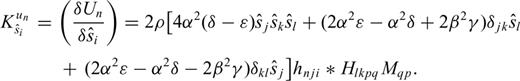
The waveform Fréchet kernel defined in eq. (3) is the fundamental formula from which Fréchet kernels of any seismic observable for any model parameter can be derived. Eqs (12–14) are general expressions for the Fréchet kernels of waveform perturbations for anisotropic parameters ɛ, δ and γ with an arbitrarily oriented axis of symmetry . In current practices of seismic anisotropy imaging studies, the most commonly encountered situation is one in which the axis of symmetry is oriented either vertically in the case of radial anisotropy or horizontally in the case of azimuthal anisotropy. In this appendix, we derive the explicit expressions of the waveform Fréchet kernels for anisotropic parameters in these two particular cases.

In eqs (12–14), assuming a vertical axis of symmetry, that is, , or 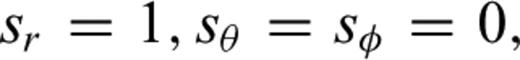we obtain the expressions of waveform Fréchet kernels for the anisotropic model parameters in a radially anisotropic reference model

(A1)

(A2)

(A3)

The Fréchet kernel of any given seismic observable can then be derived by substituting these expressions into eq. (9) and using the appropriate form of the functional for the observable.

For a reference model with azimuthal anisotropy, the axis of symmetry lies in the horizontal plane. Assuming that the azimuth of the symmetry axis is ϕ, then and 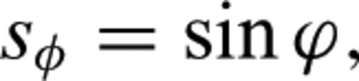and from eqs (12–14) we have

(A4)

(A5)

(A6)

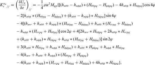
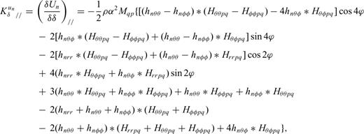
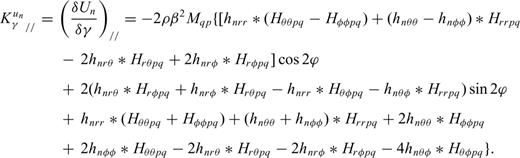
Again the Fréchet kernel of any seismic observable can be obtained by substituting these expressions into eq. (9) with the corresponding functional . The classical dependence on 4ϕ and 2ϕ (e.g. Smith & Dahlen 1973) emerges naturally in these expressions.

References