An efficient and flexible approach to the calculation of three-dimensional full-wave Fréchet kernels for seismic tomography—I. Theory

Summary

1 Introduction

All the seismic waves used in seismic tomography have a finite frequency range. It is now well recognized that wave energy is not concentrated only on the ray path, but rather spreads inside a volume, the so-called Fresnel volume, surrounding the ray. In other words, a seismic wave is influenced by, or sensitive to, the structure within a Fresnel volume, usually defined by the first Fresnel zone. However, quantitative descriptions of structural sensitivities of seismic waves were so far hindered by the computational load required for their calculation. Consequently, in the vast majority of tomographic studies, finite-frequency effects are not considered, and geometrical ray theory is used. Such an approach is only valid for imaging heterogeneities larger than the width of the first Fresnel zone. For example, the width of the first Fresnel zone of a 1-sec P wave at a distance of 90° is about 400 km in the lower mantle, which constitutes a fundamental limitation of the resolution of tomographic images unless finite-frequency effects are accounted for.

Advances in high-performance computing, coupled with developments in theoretical and numerical seismology in the past 15 yr, have provided accurate structural sensitivities of seismic waves (e.g. Woodward 1992; Yomogida 1992; Li & Tanimoto 1993; Marquering & Snieder 1995; Zhao & Dahlen 1996; Dahlen et al. 2000; Hung et al. 2000; Zhao et al. 2000; Zhou et al. 2004). These studies have demonstrated the complex sensitivities of body waves and surface waves to the different types of seismic observables. In particular, the sensitivity of seismic traveltime, the most widely used observable in structural seismology, has been shown to have a banana–doughnut shape, with zero sensitivity to the structure right on the ray path for the wave travelling directly from source to receiver (Marquering et al. 1999; Dahlen et al. 2000; Hung et al. 2000). In principle, accurate sensitivity kernels should allow us to resolve structural anomalies with spatial dimensions similar to or smaller than the first Fresnel zone width of seismic waves. Dahlen et al. (2000) introduced an efficient algorithm which made it practical to use 3-D kernels in global tomography (Montelli et al. 2004). However, the ray theory approximation adopted in Dahlen et al. (2000) is only applicable to observations from geometrical arrivals in the far-field and cannot be used to describe diffracted waves. For traveltime sensitivity kernels, Favier et al. (2004) have shown that the influence of the near field is important for distances up to one wavelength from the receiver. For regional tomography based upon phase measurements of long period surface waves (a Rayleigh wave of 100-s period has a wavelength of about 300 km), this effect can limit the resolution potential significantly. Efforts have been made more recently to develop efficient numerical methods to compute full-wave sensitivity kernels for seismic tomography based on 1-D reference models (e.g. Nissen-Meyer et al. 2007). Using the approach of Zhao et al. (2000) and Zhao & Jordan (2006) based upon normal-mode coupling to calculate complete Fréchet kernels for the phase of Rayleigh waves, Chevrot & Zhao (2007) have shown that regional surface wave tomography can indeed resolve structures as small as 100 km, smaller than the size of the first Fresnel zone. However, the application of the normal-mode approach has so far been rather limited owing to a low numerical efficiency.

Here, we propose an alternative approach to computing the 3-D kernels based on a Green function database. The main advantage of this approach is that Green's functions only depend on the reference model, thus a pre-calculated Green's function database eliminates the need for repetitive evaluations of the wavefield in 3-D kernel calculations, which considerably reduces the CPU time. This approach is analogous to computing normal-mode synthetic seismograms where a model-dependent eigenfunction table is generated, reducing the synthetic calculation to a simple summation of the eigenfunctions. Eigenfunction tables are crucial to making the normal-mode theory a practical approach in computing accurate and complete synthetic seismograms in 1-D Earth models.

In the Green's function database, the elements of the Green's tensors are calculated and stored on a set of (r, Δ) grid points. The construction of the database requires a certain amount of CPU time and disk storage depending on the problem of interest. However, the generality of the Green's tensors ensures that this approach is efficient and flexible. The computations of 3-D kernels for any phase on the seismogram (P, S, Pdiff, surface waves, etc.), for any type of data (traveltime, amplitude, splitting intensity, waveforms, etc.), and for any model parameters (isotropic, anisotropic, attenuation, etc.) only involve multiplications (in the Fourier domain) or convolutions (in the time domain) of the Green's functions retrieved from the database. The Green's tensor database can also be applied to the computations of partial derivatives with respect to source parameters for the inversions of CMT solutions and higher moments of finite sources (McGuire et al. 2001; Chen et al. 2005; Zhao et al. 2006). Large terabyte databases can be located at designated storage centres for public use in global high-resolution and regional fine-resolution studies, while individual researchers can generate small, portable and customized databases for fast inversions using single workstations or even laptops.

2 Green's Tensor and Representation Theorem

For a continuum such as the Earth, the Green's tensor G is the fundamental solution to the wave equation, that is,

1

where (r_S, t) is the spatial-temporal location of the source, δ is the Dirac-delta function and I is the second-order identity tensor. The Earth model is given by its density ρ and the fourth-order elasticity tensor Λ. Any wavefield quantity can be expressed in terms of the Green's tensor via the representation theorem (e.g. Aki & Richards 2002). In particular, for an earthquake represented by a point source at r_S and a moment tensor M, its displacement field can be expressed as

2

where ∇^S is the gradient operator acting on the source coordinates, and the symbol []²¹³ represents the transposition of the first two indices of a third-order tensor such that [A]²¹³_ijk= A_jik (Ben-Menahem & Singh 1981). Without losing generality, the time history of the moment tensor M has been assumed to be the Dirac-delta function δ (t). For a different time history, say f(t), the displacement can be obtained by convolving (2) with f(t).

3 FrÉchet Derivatives

In seismic tomography, we collect observations of anomalies or discrepancies between recorded and model-predicted seismograms. We then compute the Fréchet derivatives of seismic observables with respect to model parameters to invert the observables for the model perturbation. The fundamental quantity from which we can derive the Fréchet derivative of any type of seismic observable is the waveform Fréchet derivative. Here, we first derive the formal expression for the waveform Fréchet derivative, and then illustrate how it can be used to derive traveltime Fréchet kernels. Fréchet Kernels for other types of seismic observables are presented in a companion paper (Zhao & Chevrot 2011, hereafter referred to as Paper II).

3.1 Waveform Fréchet derivatives

The exact displacement perturbation caused by a perturbation of the reference model can be expressed in the form of the Lippmann–Schwinger equation (Lippmann & Schwinger 1950; Dahlen & Tromp 1998). Under the Born approximation, the displacement perturbation observed at a receiver located at an arbitrary location r_R can be written as (e.g. Snieder & Nolet 1987; Zhao & Dahlen 1996; Zhao et al. 2000)

3

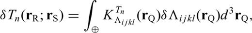
where is the gradient operator acting on the coordinates of r_Q, and the spatial integral is over the entire volume of the earth ⊕. In this section, a tilde indicates a quantity evaluated in the reference Earth model. The geometry of the locations of r_S, r_Q and r_R in the Earth and their projections on the spherical surface are illustrated in Fig. 1. In eq. (3), we only consider perturbations in the fourth-order elasticity tensor . Contributions from perturbations in density and topography of seismic discontinuities can be treated in a similar way (Dahlen 2005).

Figure 1

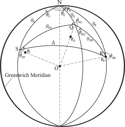
Geometry of the source at r_S, receiver at r_R, and an arbitrary location r_Q at which the Fréchet kernel is being calculated. S, R and Q are the surface projections of r_S, r_R and r_Q, respectively. Here r_R and R coincide since the receiver is assumed to be on the surface.

Open in new tabDownload slide

The τ-integral in eq. (3) gives a displacement perturbation density, that is, a displacement perturbation for a source at r_S and a receiver at r_Rcaused by a model perturbation in a unit volume around r_Q. From eq. (3), the n-component of the displacement perturbation density can be written as

4

where * denotes convolution. From eq. (4), we can immediately derive the Fréchet derivative of waveform with respect to an element Λ_ijkl of the elasticity tensor

5

In writing eq. (5), we omitted the source and receiver locations in the argument on the left-hand side to emphasize that the waveform Fréchet derivative varies with the spatial-temporal point (r_Q, t) for a given pair of source and receiver.

3.2 Traveltime Fréchet derivatives

Almost all seismic observations are obtained from linear operations of waveforms, therefore any seismic observable can be expressed as a linear functional of the displacement perturbation density δ U, and thus be linearly related to the model perturbation δΛ through eq. (4). For example, phase (or traveltime) anomalies of finite-frequency seismic records can be measured by cross-correlating synthetic and observed seismograms of a particular component

6

The lag time δ T_n of the maximum in the cross-correlagram indicates the overall delay of the record relative to the synthetic and is thus defined as the delay time. Thus we have

7

which, under the Born approximation, leads to (e.g. Dahlen et al. 2000; Zhao et al. 2000)

8

where the integral is over a certain time window [t₁, t₂] that contains the seismic phase of interest. Eq. (8) implies that the delay time obtained from the cross-correlation between synthetic and recorded waveforms of a seismic arrival is simply the integration of the waveform misfit or perturbation weighted by the time derivative of the waveform and normalized by the total power of the waveform in the selected time window. The delay time in eq. (8) can be written as (Chen et al. 2007)

9

with

10

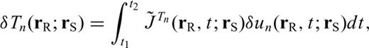
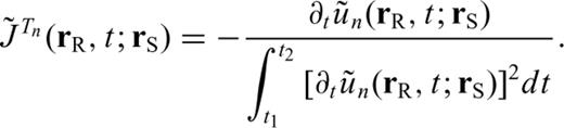
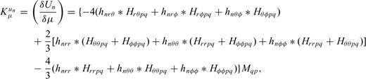
In this formulation, is a functional dependent upon the starting model as well as the particular seismic observable under consideration. In paper II, we derive these functionals for other types of seismic observables.

Substituting the total displacement perturbation in eqs (3) into eq. (9) immediately leads us to the expression for the Fréchet kernel of finite-frequency traveltime measurements

11

Therefore, we can express the traveltime Fréchet kernel for the model parameter Λ_ijkl in terms of the corresponding waveform Fréchet derivative

12

The Fréchet kernel provides a linear relationship between traveltime anomaly (delay time) and the perturbation of Earth's elastic parameters, that is,

13

which allows us to formulate a tomographic inverse problem. From eq. (5) we can see that to compute the Fréchet kernel at an arbitrary location r_Q, we only need , the earthquake-generated wavefield from source r_S to r_Q, and , the Green's tensor from r_Q to receiver r_R. Both are evaluated in the reference model.

4 FrÉchet Kernels in Terms of Strain Green's Tensors

As mentioned before, the Green's tensor is the fundamental displacement solution to the wave equation. However, a closer look at eqs (2–5) and (11) suggests that the important quantity to consider is in fact the spatial gradient of the Green's tensor, that is, strain rather than displacement. Therefore, a more useful and fundamental quantity is the third-order strain Green's tensor (SGT) at location r produced by an elementary source at r_S

14

where the symbol []²³¹ represents the transposition of a third-order tensor such that [A]²³¹_ijk= A_jki. From now on we will drop the tilde indicating the reference model for brevity. We refer to the third-order tensor h in eq. (14) as the single-side strain Green's tensor (SSGT) because it is the strain tensor at the single source side r_S. With the SSGT, the displacement field at r_Q and r_R from a moment tensor source of Dirac-delta function time history at r_S can simply be written respectively as

15

The gradient of the displacement in eqs (3–5) and (11) requires that we also define a second important quantity, the fourth-order two-side strain Green's tensor (TSGT)

16

where the symbol [ ]²¹³⁴ represents the transposition of the first and second indices of a fourth-order tensor such that [A]²¹³⁴_ijkl= A_jikl. With the TSGT, the strain field at an arbitrary receiver location r generated by an earthquake represented by a moment tensor of Dirac-delta function time history at r_S is

17

Here the superscript T denotes the transposition of a second-order tensor. Taking advantage of the symmetry properties of the elasticity tensor Λ, the spatial gradients of the Green's tensor and displacement in eqs (2–5) and (11) can be replaced by the SGTs. Thus the displacement perturbation density in eq. (4) can be written as

18

and the waveform Fréchet kernel in eq. (5) becomes

19

From eq. (19), we can proceed to derive more explicit expressions of waveform Fréchet derivatives for the elastic parameters of an isotropic medium. The perturbation of the elasticity tensor of an isotropic medium can be expressed as

20

where δκ and δμ are perturbations in the bulk and shear moduli, respectively, and the symbols δ_ij with subscripts are the Kronecker delta. Substituting eq. (20) into eq. (18), and using eq. (19), we can readily derive the expressions of waveform Fréchet kernels for the isotropic elastic moduli

21

22

where we have conveniently omitted the arguments r_Q and t. Moreover, using the relations between elastic moduli and the isotropic seismic wave speeds ρα²=κ+ 4μ/3 and ρβ²=μ, we obtain the waveform Fréchet kernels for the P- and S-wave speeds

23

24

Therefore, to compute the value of a Fréchet kernel at an arbitrary location, we only need to have two sets of quantities: the elements of the fourth-order TSGT H and the elements of the third-order SSGT h. These SGTs can be calculated in either time or frequency domain by any wave-propagation theory suitable for the 1-D or 3-D Earth model. In the rest of this paper, we discuss calculation of the SGTs by normal-mode summation and present their numerical results. Application of the SGTs in calculating Fréchet kernels will be described in Paper II.

5 Computation of SGTS by Normal-Mode Summation

Up to now, the derivations for the expressions of Fréchet derivatives are completely general. Different wavefield calculation techniques can be used to calculate the SGTs needed to compute the Fréchet derivatives. In this study, we consider the implementation of these expressions in a spherically symmetric (i.e. 1-D) reference model by the summation of normal modes. Currently, spherically symmetric Earth models are still a reasonable choice in global as well as regional tomography in which Fréchet kernels can be computed relatively efficiently. In a spherically symmetric 1-D elastic Earth model, the Green's tensor for a source located at r_S can be expressed in terms of the summation of normal-mode eigenvectors (e.g. Zhao & Dahlen 1996; Dahlen & Tromp 1998)

25

where H(t) is the Heaviside step function, a superscript ‘*’ represents complex conjugate, and ω_j is the eigenfrequency of the j-th normal mode whose eigenvector is defined as

26

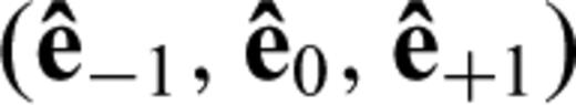
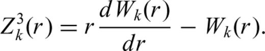
In eq. (26), Y_lm(θ, ϕ) is the complex surface spherical harmonics (SSH) of angular degree l and azimuthal order m (Edmonds 1960), is the surface gradient operator, and and are the three basis vectors of the spherical polar coordinate system. The functions U_k(r), V_k(r) and W_k(r) are radial eigenfunctions for a chosen earth model and are numerically calculated by well-established programs such as MINEOS or OBANI (Woodhouse 1988; Dahlen & Tromp 1998). There are two types of modes: spheroidal modes (S) whose radial eigenfunctions W_k(r) are identically zero, and toroidal modes (T) whose radial eigenfunctions U_k(r) and V_k(r) are both identically zero. As a result, the normal-mode summation in eq. (25) is always separated into a spheroidal-mode summation for the P–SV component waveform and a toroidal-mode summation for the SH component waveform. Due to the spherical symmetry of the reference model, the radial eigenfunctions as well as the eigenfrequencies are independent of the azimuthal order m. Thus, for simplicity, the radial eigenfunctions U_k(r), V_k(r) and W_k(r) can be identified by the single index k = (n, l) that includes the information only on the overtone number and the angular degree. Similarly, the eigenfrequency ω_j can also be denoted ω_k.

By definition the modal strain tensor ɛ_j can be written in terms of the modal eigenvector

27

Substituting eq. (25) into eq. (2), and convolving with H(t), we obtain the displacement from a moment tensor M with a Heaviside step function time history in terms of normal-mode summation (e.g. Aki & Richards 2002, eq. 8.30)

28

and the associated strain field

29

The SGTs in eqs (14) and (16) can also be written in terms of modal strains and modal eigenvectors

30

31

with

32

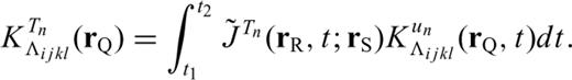
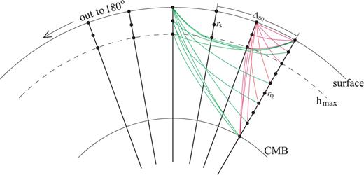
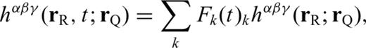
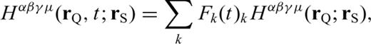
As discussed previously, to compute a Fréchet kernel we need to evaluate the waveform Fréchet kernel in eq. (19), which depends on the SSGT h and the TSGT H. At each point in space, the evaluation of the SGTs is achieved by the summation of tens of thousands of normal modes for periods of 20 s, which makes the entire calculation rather tedious. One way to reduce the computations necessary to compute the Fréchet kernels is to pre-calculate h and H on a spatial grid and store them on a disk. The required storage would be very expensive for a 3-D model since the SSGTs and TSGTs would then depend on the precise locations of source and receiver. However, for a spherically symmetric Earth model, h (r_R; r_Q) only depends on |r_R | = r₀, usually the radius of the Earth, |r_Q | = r_Q and Δ_QR, the angular distance between r_Q and r_R. Therefore, we can compute h (r_R; r_Q) for a set of (r_Q, Δ_QR) values and establish a database for h (r_R; r_Q). Fig. 2 is an illustration of the (r_Q, Δ_QR) grid in establishing the database for SSGT h (r_R; r_Q). Similarly, H (r_Q; r_S) only depends on |r_S | = r_S, the earthquake source depth, |r_Q | = r_Q, and Δ_SQ, the angular distance between r_S and r_Q. We can thus establish a database of TSGT H (r_Q; r_S) for a set of (r_S, r_Q, Δ_QR) values (see Fig. 3), which can be used in the evaluation of using eq. (19). The SGTs can be calculated using an exact full-wave method such as the normal-mode theory. Then, using the SGT database, we can compute full-wave Fréchet kernels by trivial evaluations of eq. (19). In this way, we are able to achieve accuracy with reasonable computational costs.

Figure 2

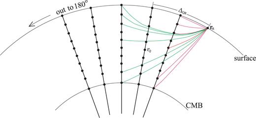
Schematic illustration of the spatial grid used in SSGT database. The receiver r_Ris fixed on the surface. For every sampling point r_Q, 10 time-series (h_i in eq. B12) are computed for the SSGT from r_Q to r_R.

Open in new tabDownload slide

Figure 3

Schematic illustration of the spatial grid used in TSGT database. For each pair of sampling points r_S and r_Q, 20 time-series (H_i in eq. B15) are computed for the TSGT. h _max indicates the maximum known depth of earthquakes and it is the maximum depth that source sampling points r_S need to reach.

Open in new tabDownload slide

In evaluating the waveform Fréchet kernel using eq. (19), since the elasticity tensor perturbation δΛ and the moment tensor M are usually given in spherical polar system with basis vectors and , the databases for the SGTs should also be calculated in the same coordinate system. However, to simplify the normal-mode expressions, we take advantage of the generalized surface spherical harmonics (GSSH) in our derivations. The classical paper by Phinney & Burridge (1973) introduced into seismology the GSSH which made the algebra involved in the analysis of wave propagation and normal modes on a spherical Earth more elegant and less tedious. The GSSH have been used in several studies based on the normal-mode theory (e.g. Woodhouse & Girnius 1982; Boschi & Woodhouse 2006; Yang et al. 2010). Dahlen & Tromp (1998) gives a thorough and very accessible discussion of the GSSH in their Appendix C. We provide a few basic definitions and formulae in Appendix A to make the discussion in the current paper more self-contained.

The normal-mode eigenvectors and modal strain tensors can be expanded in terms of the basis vectors in the generalized coordinate system

33

34

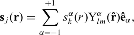
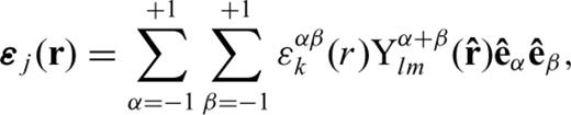
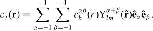
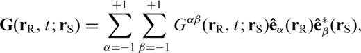
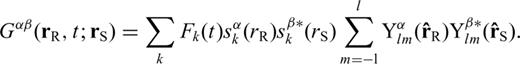
where and are the GSSH as defined in Dahlen & Tromp (1998). Expressions of the radially dependent functions s^α_k (r) and ɛ^αβ_k (r) are given in Appendix A. Hereafter, Greek letters indicate quantities in the generalized coordinate system. Given the normal-mode expansion of eigenvector and modal strain tensor in the generalized coordinate system, we can derive the expressions of the two SGTs

35

36

with the expansion coefficients in the generalized system

37

38

Upon using the addition theorem of the generalized spherical harmonics (Edmonds 1960; Li & Tanimoto 1993; Dahlen & Tromp 1998)

39

with and the quantities θ_QR, ϕ_RQ and ϕ_QR defined in Fig. 1, the expansion coefficients in eqs (37) and (38) become

40

41

where X ^N_lM (θ) is the modulus of the complex GSSH Y ^N_lM (θ, ϕ), that is, Y ^N_lM (θ, ϕ) = X^N_lM (θ) exp (iMϕ). By substituting the expressions for the radial functions s^α_k (r) and ɛ^βγ_k (r) given in eqs (A3) and (A5), respectively, into eqs (40) and (41), it is straightforward to derive the expressions for the coefficients h^αβγ (r_R, t; r_Q) and H^αβγμ (r_Q, t; r_S). Through the transformation matrix between the generalized system and the spherical polar system, we can convert the elements in generalized coordinate system h^αβγ (r_R, t; r_Q) and H^αβγμ (r_Q, t; r_S) to those in the more familiar spherical polar system h_ijk(r_R, t; r_Q) and H_ijkl(r_Q, t; r_S), respectively. Expressions for h_ijk(r_R, t; r_Q) and H_ijkl(r_Q, t; r_S) in terms of normal-mode eigenfunctions are given in Appendix B.

6 Numerical Implementation and Examples of SGTS

As shown in eqs (30) and (31), the two types of SGTs can be expressed in terms of normal-mode eigenvectors and strains. Therefore, the construction of a SGT database can be realized in two steps: (a) calculating a complete set (up to certain frequency) of normal-mode eigenfunctions for the reference model, that is, the radial functions U_k(r), V_k(r) and W_k(r) in eq. (26) for all possible k values up to the given maximum frequency; and (b) evaluating the summations in eqs (30) and (31) to obtain all elements of the SGTs. The algorithm for calculating normal-mode eigenfunctions is now well established and standard programs such as MINEOS and OBANI (Woodhouse 1988; Dahlen & Tromp 1998) are distributed and used widely by the seismological community. Although Step (b) only involves simple summations of the eigenfunctions, it can be computationally laborious when the number of grid points at which the SGTs are calculated is large. As discussed in Appendix B, even though there are 27 elements in the third-order SSGT h (r_R; r_Q) and 81 elements in the fourth-order TSGT H (r_Q; r_S), both types of SGTs have symmetry properties we can exploit such that only 10 functions in eq. (B12) for h (r_R; r_Q) and 20 functions in eq. (B15) for H (r_Q; r_S) need to be calculated and stored in the SGT database. This greatly reduces the CPU time and the storage needed to establish the SGT database.

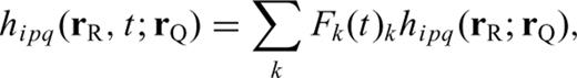
For the source-side SGTs h_ipq(r_R, t; r_Q), we calculate the 10 functions defined in eq. (B12), h₁, h₂, … , and h₁₀, between a set of grid points r_Q to a fixed receiver position r_R on the Earth's surface (see Fig. 2). The resulting SSGT portion of the SGT database is composed of the 10 functions, h₁, h₂, …, and h₁₀, sampled on a set of (r_Q, Δ_QR, t) grid points. If the region of interest is the whole mantle, we can choose r_Q to be at a series of depths from the surface down to the core–mantle boundary, Δ_QR at a set of epicentral distances from 0 out to 180°, and t up to an appropriate length of time, say 3600 s. The ranges and sampling rates of r_Q, Δ_QR and t are flexible and should be tuned depending on the particular problem of interest. For example, if one wants to compute 3-D long period surface wave kernels, a coarse time sampling (typically of a few seconds) will be sufficient for a spatial grid covering the upper mantle only. With an average sampling interval of ∼20 km in r_Q and uniform sampling rates of 0.2° in Δ_QR and 1 s in time, it takes ∼100 hr on a cluster with 20 2.5 GHz processors to compute the 2400-s long SSGTs for the whole mantle by summing normal modes up to 0.3 Hz, and the total disk space to store the SSGT portion of the database is ∼12 GBytes. Two examples of the SSGT are shown in Figs 4 and 5. In all the numerical examples shown in this study we have used model PREM (Dziewonski & Anderson 1981). Plotted in Figs 4 and 5 are the physically more meaningful h_ipq(r_R, t; r_Q) defined in (B11), with both r_Q and r_R on the equator and r_R positioned to the east of r_Q. In this configuration, the time-series in Fig. 4 are obtained from (B11) using ϕ_RQ=π/2 and the 10 h_i(t) time-series for r_Q= 6371 km and Δ_QR= 30° extracted from the SSGT database. The time-series in Fig. 5 are obtained in the same way with r_Q= 6330 km. Of the 18 independent elements in h_ipq(r_R, t; r_Q), only those with significant amplitudes are plotted. All other elements have negligibly small maximum amplitudes. The time-series in Figs 4 and 5 clearly resemble seismograms. By definition, an element h_ipq(r_R, t; r_Q) represents the time-series of the ith component of displacement at r_R caused by the (p, q)-element of strain at r_Q. In fact, an immediate application of the SSGT is the calculation of synthetic seismograms, since the ith component of the displacement caused by a moment tensor M is simply the product M_pqh_ipq(r_R, t; r_Q). Figs 6 and 7 show the synthetic seismograms at r_R due to a double-couple source at r_Q positions in Figs 4 and 5, respectively. To check the accuracy of the SSGT database, we also compared them to synthetic seismograms calculated by standard normal-mode summation procedure. The results are in perfect agreement with those obtained with the SSGT database.

Figure 4

Numerical examples of the SSGT h_ipq(r_R, t; r_Q), with both r_Q and r_R on the equator and r_R positioned to the east of r_Q. r_Q is located on the surface. All time-series have been filtered by a four-pole Butterworth bandpass filter with corner frequencies at 0.002–0.08 Hz and are plotted with the same vertical scale. Only elements with significant amplitudes are plotted.

Open in new tabDownload slide

Figure 5

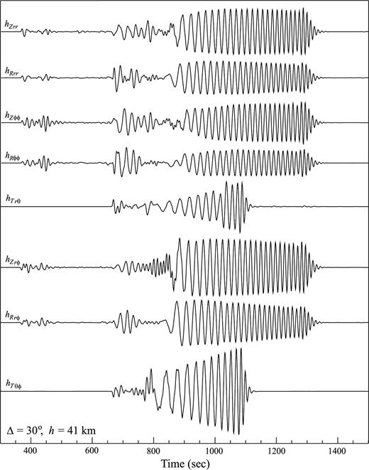
Numerical examples of the SSGT h_ipq(r_R, t; r_Q), with both r_Q and r_R on the equator and r_R positioned to the east of r_Q. r_Q is located at a depth of 41 km. All time-series are filtered by a 4-pole Butterworth bandpass filter with corner frequencies at 0.002–0.08 Hz and are plotted with the same vertical scale. Only elements with significant amplitudes are plotted.

Open in new tabDownload slide

Figure 6

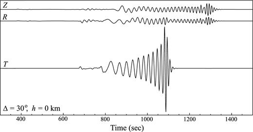
Synthetic seismograms obtained from the SSGTs in Fig. 4. A point source with a focal mechanism of 60°/45°/45° for strike/dip/rake angles has been used. The source time function is such that the moment tensor is a Heaviside function in time.

Open in new tabDownload slide

Figure 7

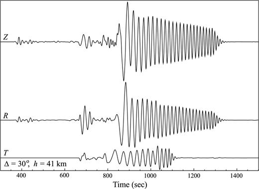
Synthetic seismograms obtained from the SSGTs in Fig. 5. A point source with a focal mechanism of 60°/45°/45° for strike/dip/rake angles has been used. The source time function is such that the moment tensor is a Heaviside function in time.

Open in new tabDownload slide

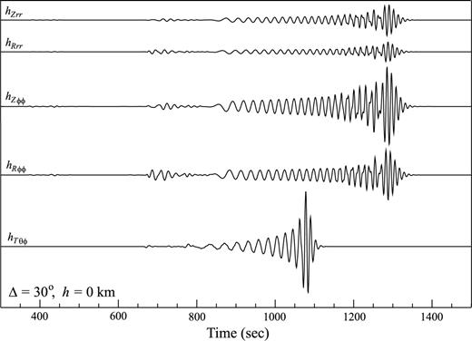
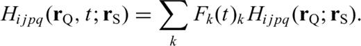
The SSGT part of the SGT database requires relatively less computation and disk space because only 10 functions h₁, h₂, … , and h₁₀ are involved and the receiver r_R is fixed on the surface. The TSGTs, however, require the calculation of 20 functions H₁, H₂, … , and H₂₀ in (B15) that need to be stored on a 4-D grid (r_S, r_Q, Δ_SQ, t). The values of r_Q and t can be the same as those for SSGT, and Δ_SQ can also be sampled on the same grid as that for Δ_QR. The depth samples for r_S may be limited to 700 km, the maximum possible depth of earthquakes. With the similar sampling parameters for (r_Q, Δ_SQ, t) to those for the SSGT discussed before but a finer grid size for r_S (a total of about 100 samples down to 700-km depth), it takes ∼1000 hr on the same cluster with twenty 2.5 GHz processors to compute the 2400-s long TSGTs for the whole mantle by summing normal modes up to 0.3 Hz, for a total storage volume of ∼1.2 TBytes. Fig. 8 shows examples of the TSGT time-series H_ijpq(r_Q, t; r_S), with both r_S and r_Qon the equator and r_Q positioned to the east of r_S. Therefore, the TSGTs in Fig. 8 are obtained from (B14) using ϕ_QS=π/2, ϕ_SQ= 3π/2 and the 20 H_i(t) time-series for r_S= 6334 km, r_Q= 6371 km and Δ_SQ= 30° extracted from the TSGT database. Similar to the SSGTs in Figs 4 and 5, many of the TSGT elements have negligibly small amplitudes for this r_S and r_Q configuration and are not plotted.

Figure 8

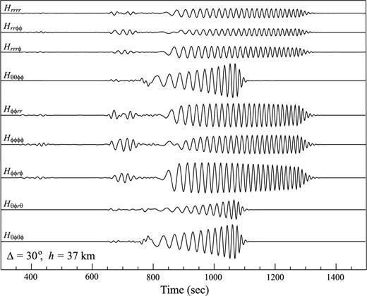
Numerical examples of the TSGT H_ijpq(r_Q, t; r_S), with both r_S and r_Q on the equator and r_Q positioned to the east of r_S. r_S is located at a depth of 37 km, and r_Q is on the surface. All time-series have been filtered by a four-pole Butterworth bandpass filter with corner frequencies at 0.002–0.08 Hz and are plotted with the same vertical scale.

Open in new tabDownload slide

Another way to visualize the spatial variation of the SGTs is to look at their snapshots. In Fig. 9, the SSGT component h_Tθϕ in the great-circle plane is displayed for the time instants of 400 s, 800 s, 1200 s and 1600 s. From eq. (15) the transverse-component displacement at r_R, u_T(r_R, t; r_Q), is proportional to the SSGT element h_Tθϕ(r_R, t; r_Q) at r_Q. The proportionality factor is simply the moment tensor element M_θϕ. Therefore, a snapshot at time t_i represents the amplitude of the transverse-component displacement at r_R and t_i generated by a unit impulsive moment tensor element M_θϕ= 1 at r_Q. It is thus expected that the snapshots in Fig. 9 resemble those of SH-wave fronts emanating from a strike-slip source (e.g. fig. 3.5–19 of Stein & Wysession 2003) at location r_R. Fig. 10 shows snapshots for the h_Zrr component (eq. B11a). The pattern resembles the wave fronts of the P–SV system. Other elements of the SSGT h (r_R, t; r_Q) can be viewed and interpreted in the same way. For a specific element of the TSGT H (r_Q, t; r_S), the snapshots will represent the strain, or spatial gradients of the displacement, at r_Q and time t, due to a specific element of the moment tensor of unit strength at r_S.

Figure 9

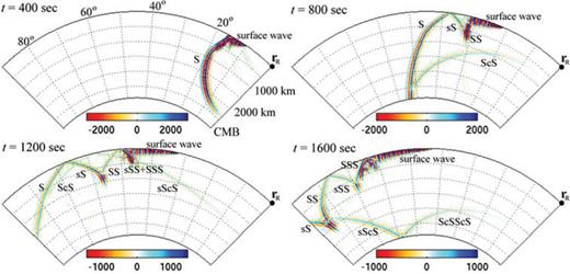
Snapshots of the SSGT h_Tθϕ(r_R, t; r_Q) taken at 400 s, 800 s, 1200 s and 1600 s. Receiver location is fixed at r_R. Plotted here are the values of h_Tθϕ(r_R, t; r_Q) normalized by a factor of 0.952 × 10⁻²⁵N⁻¹.

Open in new tabDownload slide

Figure 10

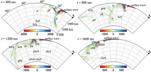
Snapshots of the SSGT h_Zrr(r_R, t; r_Q) taken at 400 s, 800 s, 1200 s and 1600 s. Receiver location is fixed at r_R. Plotted here are the values of h_Zrr(r_R, t; r_Q) normalized by a factor of 0.952 × 10⁻²⁵N⁻¹.

Open in new tabDownload slide

7 Conclusions

We have shown that by defining the third-order SSGT and the fourth-order TSGT, we can express the perturbation to the displacement from source r_S to receiver r_R induced by the heterogeneity in structure at an arbitrary location r_Q in terms of the convolution between the SSGT from r_S to r_Q and the TSGT from r_Q to r_R. By exploiting the fact that the SSGT and TSGT only depend on the reference Earth model, we can pre-calculate and establish a database of the SGTs from which the synthetic seismograms as well as the Fréchet kernels can be evaluated more efficiently. This provides a possibility of conducting full-wave seismic tomography using the non-geometrical seismic signals that cannot be modelled by asymptotic ray theory.

We have derived the expressions of the SSGTs and TSGTs in the context of normal-mode theory and discussed the practical issues in creating a SGT database for the calculation of Fréchet kernels for tomographic studies. In the most general case, the SSGT database consists of 10 time-series distributed on a (r_Q, Δ_QR) grid; whereas the TSGT database is composed of 20 time-series distributed on a (r_S, r_Q, Δ_SQ) grid. Both the CPU time and disk space needed in calculating and storing the SGT databases are modest. However, the resulting SGT databases enable much more efficient evaluations of Fréchet kernels for tomographic inversions. In Paper II, we will describe the process of deriving the expressions of various kinds of Fréchet kernels in terms of the SGTs and present numerical examples of the kernels to demonstrate the flexibility and efficiency of the SGT approach for applications in seismic tomography.

Acknowledgments

The authors wish to thank Marie Calvet for comments that helped improve the manuscript. Numerical computations have been performed on the HPC clusters at Institute of Earth Sciences, Academia and National Center for High-performance Computing (NCHC) in Taiwan. LZ has been supported by the National Science Council (NSC) of Taiwan under grants NSC95–2119-M-001–063 and NSC96–2116-M-001–011.

Appendices

Appendix A: Normal-Mode Expressions Using Generalized Surface Spherical Harmonics

Here, we provide a few basic expressions of normal-mode solutions in terms of GSSH. Most of the materials here can be found in appendix C of Dahlen & Tromp (1998).

The complex lower canonical basis vectors are defined in terms of the three basis vectors and in spherical polar coordinate system

(A1)

In this basis, the normal-mode eigenvector can be written as

(A2)

where is the (scalar) generalized surface spherical harmonic. The radial functions s^α_k (r) can be related to the normal-mode radial eigenfunctions

(A3)

Similarly, the modal strain can also be expressed in terms of the canonical basis vectors

(A4)

with

(A5)

where the l-dependent coefficient d_l is

(A6)

and the radial functions Zⁱ_k (r) are defined in terms of the modal eigenfunctions

(A7)

(A8)

(A9)

The Green's tensor can also be expressed in terms of the generalized basis vectors

(A10)

where the coefficients G^αβ (r_R, t; r_S) can be obtained by substituting eq. (A2) into eq. (25)

(A11)

Analogous to the regular SSH, the complex GSSH can also be factorized into the product of a θ-dependent (real) generalized Legendre function and a ϕ-dependent exponential

(A12)

In computing the Fréchet kernels for seismic tomography, we only need the GSSHs with − 2 ≤α≤ 2. Therefore, a practical approach in computing the generalized Legendre functions and the GSSH is to start from P^α_2m (cos θ) and P^α_3m (cos θ), and using the recursive relation

(A13)

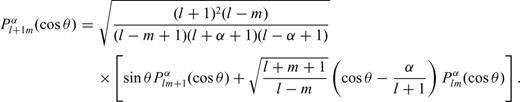
Explicit expressions for P^α_2m (cos θ) and P^α_3m (cos θ) can be found in many mathematical handbooks such as Abramowitz & Stegun (1964).

Appendix B: Expressions for Strain Green's Tensors and Their Normal-Mode Incarnations

The explicit expressions for the elements of the strain Green's tensors in the generalized system, h^αβγ (r_R, t; r_Q) and H^αβγμ (r_Q, t; r_S), are given in eqs (40) and (41). They can be written as

(B1)

(B2)

in the generalized coordinate system, with the time-independent functions

(B3)

(B4)

The spherical-polar coordinate system version of eqs (B1) and (B2) are

(B5)

(B6)

Substituting the expressions for the modal eigenfunctions s^α_k (r) in (A3) and those for the modal strains ɛ^αβ_k (r) in (A5) into (B3) and (B4), we can derive the expressions for the elements in the generalized system h^αβγ (r_R, t; r_Q) and H^αβγμ (r_Q, t; r_S). Then, these SGT elements in the generalized coordinate system can be converted to the spherical polar coordinate system through the relations

(B7)

(B8)

where and , and the transformation matrix is

(B9)

In spherically symmetric 1-D reference models, the toroidal and spheroidal modes are decoupled. Therefore, the two types of modes can be computed and summed separately. The contributions from the two types of modes are then combined to form the individual elements of h_ipq(r_R; r_Q) and H_ijpq(r_Q; r_S). The elements of h_ipq(r_R; r_Q) can be further projected onto the vertical, longitudinal (radial) and transverse components using the relations

(B10)

where and are unit vectors in vertical, longitudinal and transverse polarizations, respectively.

The expressions for the 27 elements of the SSGT h_ipq(r_R, t; r_Q) are

(B11a)

(B11b)

(B11c)

The 10 azimuth-independent coefficients h_i(r_R, t, r_Q, θ_QR) are the ones need to be calculated and stored in the SSGT database (r_R≡ 6371 km). They can be written in terms of normal-mode summation

(B12)

with the time-independent functions

(B13)

The expressions for the 81 elements of the TSGT H_ijpq(r_Q, t; r_S) are

(B14a)(B14b)

(B14c)

(B14d)

(B14e)

(B14f)

The 20 azimuth-independent coefficients H_i(r_Q, t, r_S, θ_SQ) are calculated and stored in the TSGT database. They can also be expressed in terms of normal-mode summation

(B15)

with the time-independent functions

(B16)

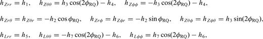
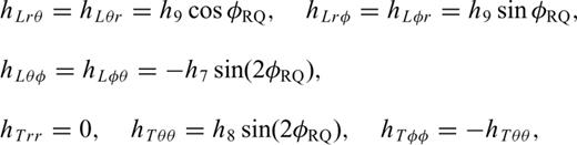
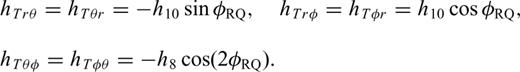
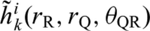
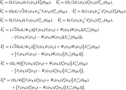
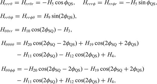
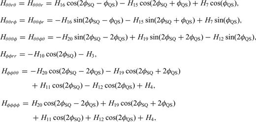
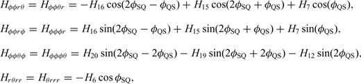
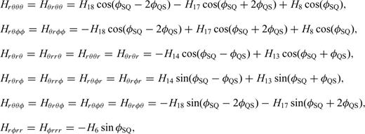
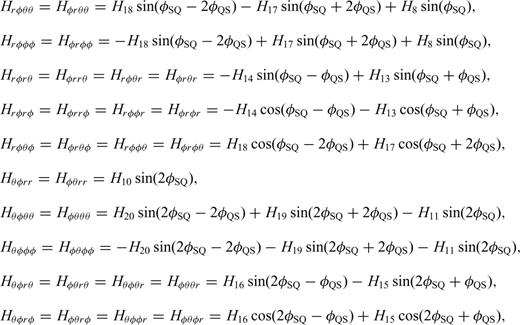
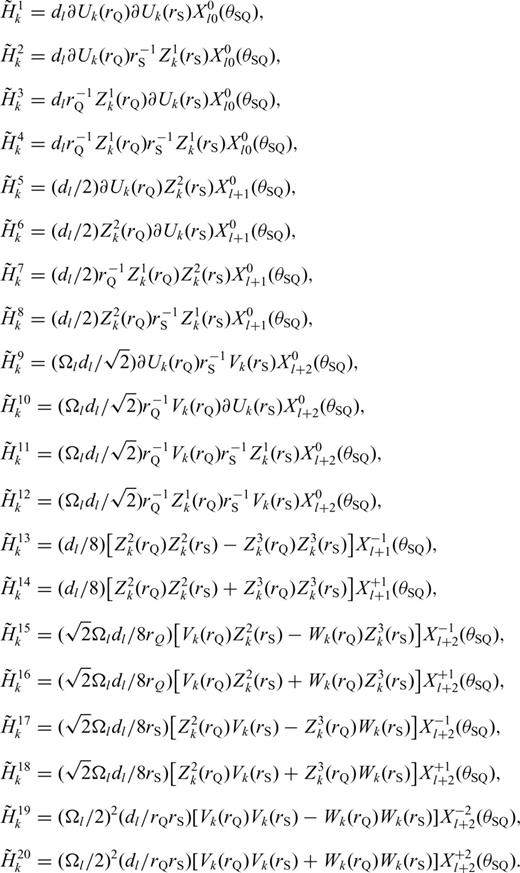
With these definitions, we only need to compute and store the 10 coefficients in eq. (B12) to obtain the 21-element third-order SSGT h_i(r_R, t;r_Q, θ_QR) in eq. (B11), and the 20 coefficients in eq. (B15) to obtain the 81-element fourth-order TSGT H_i(r_Q, t;r_S, θ_SQ) in eq. (B14).

References