Acoustic, elastic and poroelastic simulations of CO₂ sequestration crosswell monitoring based on spectral-element and adjoint methods

Summary

1 Introduction

Geologic sequestration of CO₂, a green house gas, represents an effort to reduce the large amount of CO₂ generated as a by-product of fossil fuel combustion and emitted into the atmosphere. This process of sequestration involves CO₂ storage deep underground. There are three likely storage options: injection into hydrocarbon reservoirs, injection into methane-bearing coal beds or injection into deep saline aquifers, that is, into highly permeable porous media.

In this study, we focus on storage into saline aquifers, which offer potentially large storage volumes and have been under a certain amount of scrutiny, with examples such as Sleipner, North Sea, Nagaoka, Japan, and Frio, Texas. Moreover, it simplifies modelling to use a single-fluid saturated porous medium, as opposed to a hydrocarbon reservoir containing a mixture of oil, gas and water. This level of complexity is unnecessary for our discussion, but may be readily accommodated.

Previous research has shown that it can be difficult to obtain quantifiable results using seismic reflection (e.g. Arts et al. 2004; Chadwick et al. 2009). That is why we investigate crosswell seismic imaging, which is a much better alternative for accurately monitoring injected CO₂. This approach is, however, limited to imaging an injection solely between two wells, one carrying receivers and the other sources, but it nevertheless is a very popular technique.

Storage areas are highly porous media. However, a common strategy is to perform time-lapse seismic imaging in acoustic or elastic models, using Gassmann's formulae (Gassmann 1951) to account for saturation effects (e.g. Brinks & Fanchi 2001; Arts et al. 2004). To our knowledge, in this context the only work based on Biot's poroelastic theory (Biot 1956a) is by Carcione et al. (2006), who present an extensive study describing the physics of the CO₂ storage zone, taking the Sleipner field in the North Sea as an example. Carcione et al. (2006) present time-lapse reflection surveys showing the importance of saturation within the aquifer on synthetic seismic sections.

In this paper, we investigate the influence of the theory used to model the storage zone, namely, acoustic, elastic or poroelastic, on the accuracy of imaging. We present 4-D seismic poroelastic imaging and model updates using an adjoint method, extending work by Tape et al. (2009, 2010) to image the southern California crust, and work in salt dome imaging for exploration geophysics by Luo et al. (2009) and Zhu et al. (2009). Poroelastic inverse problems are seldom addressed. Recently, De Barros et al. (2010) focused on poroelastic full waveform inversion in stratified media based on Biot theory, while Berryman & Nakagawa (2010) discussed inversion for poroelastic drained constants based on undrained ultrasound measurements using Gassmann theory.

Finally, we investigate differences between using only the direct compressional wave, as is commonly done, versus using both direct compressional and shear waves to constrain injected CO₂, as a first step towards full waveform inversion.

2 Model Setup and Poroelastic Signature

In this section, we present the model geometry, as well as synthetic seismograms calculated to define our ‘true’ data, as observed before (labelled BSL) and after injection (labelled INJ) of CO₂. We use a setup as encountered, for example, in the pilot sites of Nagaoka, Japan, (Saito et al. 2006; Onishi et al. 2009) and Frio, Texas, (Daley et al. 2007, 2008; Doughty et al. 2008), involving a slightly dipping aquifer sealed between two caprock layers (see Fig. 1). Caprock is assumed to be elastic, since we do not expect a high porosity in these sealing layers, whereas the aquifer is modelled using poroelastic theory. The properties of the different layers may be found in Table 1. For completeness and reference, the governing equations are summarized in Appendix A.

Figure 1

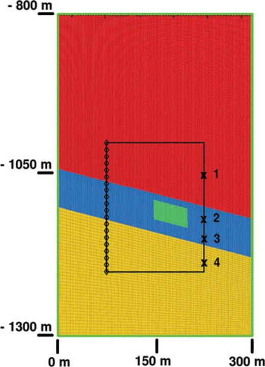
‘True’ model geometry. The brine-saturated aquifer is denoted by the blue layer sandwiched between the red and yellow caprock layers. CO₂ is injected into the green region. All edges of the model are absorbing boundaries. The diamonds correspond to 20 receivers and the crosses label four sources. All subsequent figures zoom in on the black rectangle.

Open in new tabDownload slide

Table 1

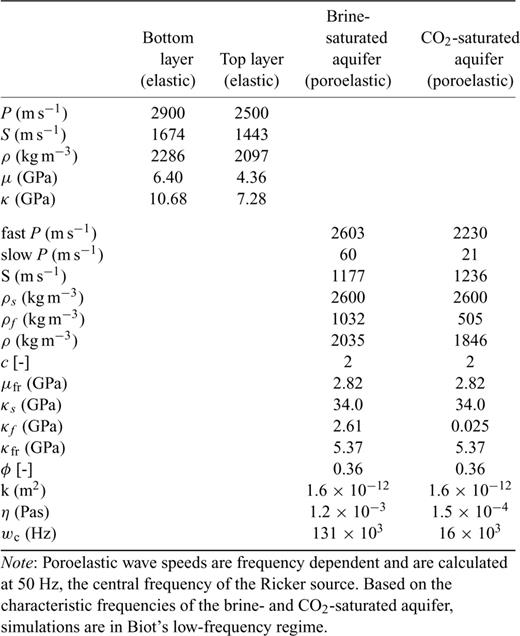
Model parameters used to generate the ‘data’.

Open in new tabDownload slide

We mimic injection of CO₂ by changing the properties of a rectangular area within the aquifer (see Table 1 and Fig. 1). Our approach is based on a single-fluid, fully saturated porous medium. Partial saturation may be incorporated, but this is beyond the scope of this paper and does not affect our main conclusions. For a detailed discussion of saturation effects the reader is referred to Carcione et al. (2006). As may be observed in Table 1, injection of CO₂ is treated by prescribing different fluid bulk modulus, density and viscosity values than those of brine present in the aquifer before injection (we used values determined by Carcione et al. (2006) for the Sleipner field). This naturally leads to changes in the fast compressional, slow compressional and shear wave speeds.

Note that the depth of injection is around 1100 m. At that depth, CO₂ is in a supercritical state, that is, in a dense and liquid-like state, leading to measurable wave speed anomalies after injection (Xue & Ohsumi 2004). In our case, changes in fluid properties contribute to changes of approximately −12 per cent for the fast P wave speed, in agreement with the literature, −65 per cent for the slow P wave speed, +5 per cent for the S wave speed and −9 per cent for the bulk density.

An array of 20 receivers and an array of four sources are deployed on either side of the injection area, facilitating the collection of crosswell seismic data (Fig. 1). The source time function is a Ricker wavelet with a dominant frequency of 50 Hz. This is towards the lower end of the typical frequency bandwidth used in crosswell acquisition, for example, 70–350 Hz (Daley et al. 2008) and 200–1000 Hz (Spetzler et al. 2008). Biot's characteristic frequencies for brine- and CO₂-saturated aquifers (see Table 1) are much larger than the 50–1000 Hz frequency range, placing crosswell acquisition in Biot's low-frequency regime, where the slow P wave exhibits diffusive behaviour (Biot 1956a). Therefore, one cannot expect to observe any direct slow P waves, but attenuation of fast P and S waves due to conversion into slow P waves as well as slow P conversion into fast P and S waves near sources may be detected (Geertsma & Smit 1961).

Crosswell seismic imaging for reservoir characterization and CO₂ sequestration monitoring is predominantly based on direct P waves. Most downhole source apparatuses are volumetric sources. Although, S waves may be observed as mode conversions, their energy is generally weak. There are, however, obvious advantages to using both P and S waves. This motivated the study of borehole sources capable of generating both P and S waves (e.g. Lee & Balch 1982; Gibson 1994; Daley & Cox 2001; Daley et al. 2004; Leary & Walter 2005) and multicomponent seismic recording to enhance direct P and S wave identification (e.g. Angerer et al. 2002; Davis et al. 2003; White 2009). To discuss the implications of using only direct P waves versus both P and S waves, we use a source which generates P and S waves of comparable energy. For acoustic simulations we use an explosive source.

Before discussing the inversion results, we generate three types of synthetic data to compare to our ‘true’ data, to highlight poroelastic signatures in the data set. To do so, we model the brine-saturated aquifer before (BSL) and after the injection of CO₂ (INJ) using different types of rheologies (see Table 2):

Table 2

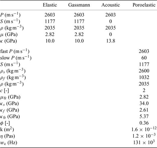
Baseline model parameters for the brine-saturated aquifer.

Open in new tabDownload slide

• (i)

  The aquifer is modelled as an elastic medium, where the compressional and shear wave speeds are identical to the fast P and S waves listed in Table 1.

• (ii)
  Gassmann's formulae are used to characterize the aquifer. These formulae relate effective bulk and shear moduli of dry rock, κ_fr and μ_fr, to effective moduli of the same rock saturated with fluid, κ_sat and μ_sat, via

  

  1

  where

  

  Here, the solid bulk modulus is denoted by κ_s, the fluid bulk modulus by κ_f and the porosity by ϕ. An elastic theory based upon these moduli is used to treat the problem. To derive the saturated moduli for the aquifer, saturated with brine and CO₂, we use the same fluid, solid and frame properties listed in Table 1. Note how Gassmann P and S wave speeds and moduli are identical to the elastic case (i) (see Table 2). This is a direct consequence of the low-frequency regime in which we operate. For that reason, in the following we only show the ‘Gassmann elastic’ results, with the understanding that in the low-frequency regime these are equivalent to the elastic case (i). Note that in the high-frequency regime the Gassmann and poroelastic theories differ. In that case, we observe discrepancies between the Gassmann and elastic cases, since P and S wave speeds in the elastic case (i) are identical to the fast P and S wave speeds in the poroelastic case.
• (iii)

  The aquifer is modelled as an acoustic layer, where the compressional wave speed is identical to the fast P wave speed listed in Table 1, but in this case there are no shear waves.

Fig. 2 shows the solid displacement time-series recorded at receiver 10 for event 2, situated at 1120 m depth inside the aquifer (see Fig. 1). The direct (fast) P and direct S arrivals are observed together with various reflected phases. A comparison is made between ‘true’ data (generated using the full poroelastic theory) and seismograms obtained using an elastic rheology based on Gassmann's formulae (‘Gassmann elastic’) and an acoustic theory to model the brine- and CO₂-saturated aquifer (first and third columns). We observe discrepancies between different models, which are emphasized by examining differences between seismograms (second and fourth columns).

Figure 2

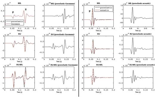
Comparison of horizontal-component displacements recorded by receiver 10 due to source two located inside the aquifer, as shown in Fig. 1. First row: comparison between poroelastic ‘data’ (black line) and Gassmann elastic (red line) simulations (first panel) and their difference (second panel), and between poroelastic data (black line) and acoustic (red line) simulations (third panel) and their difference (fourth panel) for the baseline (BSL), that is, before injection of CO₂. The Gassmann elastic simulations are equivalent to the elastic case in Biot's low-frequency regime, as discussed in the main text. Second row: comparison between poroelastic ‘data’ (black line) and Gassmann elastic (red line) simulations (first panel) and their difference (second panel), and between poroelastic data (black line) and acoustic (red line) simulations (third panel) and their difference (fourth panel) after the injection of CO₂ (INJ). The third row shows differences between seismograms recorded after injection and the baseline, thus highlighting the CO₂ signature and identifying discrepancies introduced by the Gassmann and acoustic approximations. Note the differences in vertical scale.

Open in new tabDownload slide

The first column in Fig. 3 shows the solid displacement time-series recorded at all 20 receivers for event 2. We present a comparison between the ‘true’ data and the Gassmann elastic model. From top to bottom, the three panels present differences between seismograms obtained with both theories before injection (BSL), after injection (INJ) and the difference between injection and baseline (INJ-BSL). We observe that the signal recorded before injection is not strongly affected by the choice of rheology. Significant discrepancies appear after injection of CO₂ for the S arrival and for the (fast) P arrival.

Figure 3

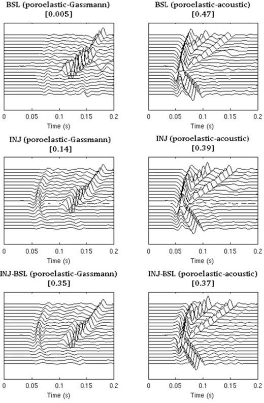
Comparison of horizontal-component displacements recorded by an array of 20 receivers due to source two located inside the aquifer, as shown in Fig. 1. The ‘data’ are generated using poroelastic simulations; these are compared to Gassmann elastic (first column; equivalent to the elastic case in Biot's low-frequency regime), and acoustic simulations (second column). The top row shows the differences between the data and Gassmann elastic simulations (first panel), and the data and acoustic simulations (second panel) before injection (BSL), thereby illustrating theoretical limitations due to various modelling approximations. The second row shows differences between the data and Gassmann and acoustic modelling approximations after CO₂ injection (INJ). The third row shows the differences between the seismograms after injection and the baseline, thus highlighting CO₂ signatures in the data and discrepancies from this signature introduced by the Gassmann and acoustic approximations. All plots are normalized, and the numbers in square brackets indicate the ratio between the maximum amplitude of the displayed differences and the maximum amplitude of the corresponding data.

Open in new tabDownload slide

The second column of Fig. 3 shows a comparison between the data and an acoustic rheology. Note that since the source is explosive, only P and P-to-S converted waves are strong enough to be observed.

We conclude that there is a poroelastic signature present in the data that cannot be captured when using an acoustic or an elastic (with or without Gassmann's formulae) rheology. These discrepancies vary in significance from one model to another, and can play a more or less significant role in imaging and inversion, as we discuss next. It is important to note that the simulations presented here are noise free. Future work on real data is required to precisely quantify poroelastic signatures relative to the signal-to-noise ratio.

3 Time-Lapse Crosswell Imaging and Model Updating

In this section, we use traveltime and amplitude anomalies to define a misfit function measuring discrepancies between data and synthetics. Associated with this misfit we derive finite-frequency sensitivity kernels, which are used to iteratively image the position of injected CO₂.

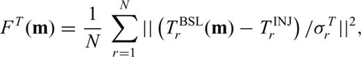
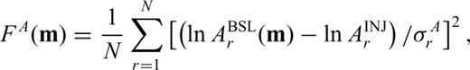
3.1 Misfit functions

To quantify the traveltime anomaly generated by the presence of injected CO₂, we introduce the traveltime misfit function (Tape et al. 2010)

2

where T^BSL_r (m) refers to the predicted cross-correlation traveltime at receiver r for model m before injection of CO₂, which constitutes the baseline, while T^INJ_r is the observed cross-correlation traveltime after injection of CO₂. In practice there may be multiple components and ‘picks’ associated with a given receiver. Similarly, we may choose to measure the misfit between the amplitudes. In that case, we introduce the amplitude misfit function (Dahlen & Baig 2002; Tromp et al. 2005)

3

where A^BSL_r (m) and A^INJ_r are cross-correlation amplitudes at receiver r predicted for model m before injection of CO₂ and observed after injection of CO₂, respectively. Here σ^T_r and σ^A_r denote standard deviations associated with the traveltime and amplitude anomaly measurements (see Appendix A in Tape et al. (2010) on the estimation of σ^T_r and σ^A_r). The implication is that when data are fitted to within their standard deviations, F^T and F^A approach 1 (note the 1/N normalization factor, where N corresponds to the total number of measurements). When fitting traveltime and amplitude anomalies together, one has to consider the following misfit

4

such that F approaches 1 when the traveltimes and amplitudes are fit to within one standard deviation.

We imagine that in practice the baseline model is obtained first, using, for example, well-log data and a series of inversions to accurately reproduce the baseline data, before tackling CO₂ imaging. Therefore, in this study the baseline model is our starting model.

We choose to express misfit kernels in terms of bulk sound wave speed, c, shear wave speed, c_s and bulk density, ρ. A discussion on the choice of model parameters may be found in Tromp et al. (2005) and Zhu et al. (2009). The bulk sound wave speed, c, is defined for the four different types of rheology as

• 1

  in the acoustic case (see Section A1),

• 2

  in the elastic case (see Section A2),

• 3

  in the Gassmann elastic case, where ρ= (1 −ϕ) ρ_s+ϕρ_f and κ_e=κ_sat, as defined in eq. (1),

• 4

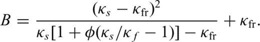
  in the poroelastic case, where ρ= (1 −ϕ) ρ_s+ϕρ_f and B is a Biot coefficient (see Section A3).

The associated misfit kernels are given by

5

6

7

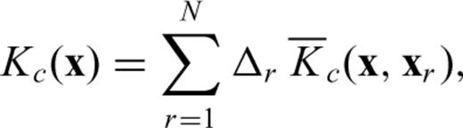
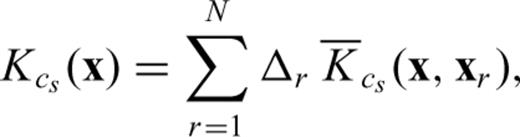
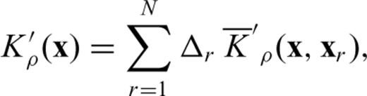
where Δ_r= (T^BSL_r−T^INJ_r)/(σ^T_r)² for traveltime misfit kernels and Δ_r= (ln A^BSL_r− ln A^INJ_r)/(σ^A_r)² for amplitude misfit kernels. The kernels are the famous ‘banana–donut’ kernels (Dahlen et al. 2000) calculated for each source–receiver combination. Note how misfit kernels are a sum of banana–doughnut kernels weighted by the measurements. For detailed definitions of the finite-frequency sensitivity kernels for elastic, acoustic and poroelastic parameters, the reader is referred to Tromp et al. (2005), Liu & Tromp (2006, 2008) and Morency et al. (2009).

3.2 Model update strategy

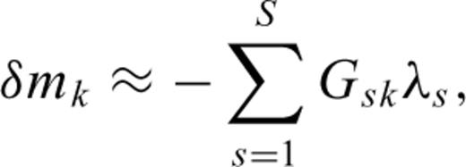
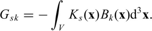
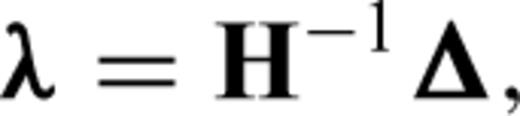
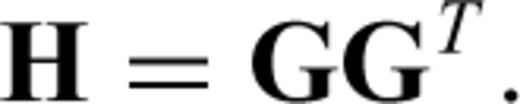
Finite-frequency sensitivity kernels are used to iteratively improve our model, better characterize the injected CO₂ area and recover storage reservoir properties. This is accomplished by minimizing the misfit functions (2), (3) or (4) using classical gradient-based (Tarantola 1984) or Hessian-based methods.

Here, we approach the inverse problem based upon a source-subspace projection method, the details of which may be found in Sambridge et al. (1991) and Tape (2009). Suffice it to say that the model update is expressed as

8

where S denotes the number of sources and G_sk an element of the source-projected gradient matrix given by

9

The event kernel K_s is defined by (5)–(7), and B_k(k= 1, … ,M) are a set of orthonormal basis functions in which we choose to expand our model. Finally, the S-dimensional vector λ plays the role of a weight for each gradient. It is determined by

10

where Δ is the projected data vector and H is the approximate S×S Hessian matrix

11

For each iteration, we choose a step length such that the maximum values of ln(m_k+1/m_k) are less than ∼10 per cent.

Updating the bulk sound wave speed in the acoustic, elastic and Gassmann elastic cases leads to simply updating the bulk modulus κ. Note, however, that in the poroelastic case this corresponds to updating the Biot coefficient

12

We make the assumption that injection of CO₂ does not affect the grains (κ_s) or the skeleton (κ_fr), but only the fluid (κ_f) (see Table 1). The variation of the misfit function with respect to the Biot coefficient B is therefore only due to changes in the fluid bulk modulus κ_f. Note that in the Gassmann elastic case we may recover fluid properties, such as κ_f, using relationship (1).

4 Results

We perform three kinds of inversions using acoustic, elastic, Gassmann elastic or poroelastic simulations:

• (i)

  direct P-wave traveltime anomalies, which is the most common approach (e.g. Saito et al. 2006; Spetzler et al. 2008; Onishi et al. 2009),

• (ii)

  direct P- and S-wave traveltime anomalies, and

• (iii)

  direct P- and S-wave traveltime and amplitude anomalies.

In this section, we discuss the results of these inversions followed by a corresponding misfit analysis. Note that the starting models, m₀₀, have the properties listed in Table 2 for the four different types of rheologies. The elastic case (i) and Gassmann elastic case (ii) will give similar results, as previously mentioned. The starting model corresponds to the model before injection of CO₂, that is, the baseline. This baseline may be established by performing a crosswell inversion prior to injection, for example.

4.1 Inversions

By measuring cross-correlation traveltime anomalies between the ‘data’ and synthetics calculated using acoustic, Gassmann elastic and poroelastic models (with properties listed in Table 2), at each iteration, we calculate the corresponding gradient of the misfit function using the kernels (5)–(7). As illustrated in Fig. 4 for the poroelastic case, P-wave traveltime inversions converge after about four iterations, at which point the gradients become small. A similar number of iterations is required for the Gassmann elastic inversion. For the acoustic case, the inversion converges after two iterations.

Figure 4

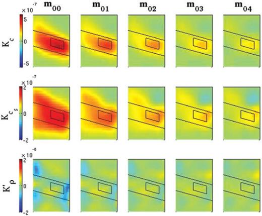
Evolution of fast bulk sound wave Fréchet derivative K_c, the shear wave derivative and the impedance derivative K′_ρ (top, middle and bottom rows, respectively) from the initial model m₀₀ (first column) through model m₀₄ (fifth column) for a poroelastic inversion using direct P-wave traveltime anomalies. Note how the amplitude of the gradient decreases with each subsequent iteration. A similar number of iterations is required for acoustic, elastic and Gassmann elastic inversions.

Open in new tabDownload slide

The main results of this research are summarized in Figs 5 and 6, illustrating our ability to recover images and properties of injected CO₂ based on various combinations of theories and data sets. The recovery of the fast P wave speed anomaly induced by injection of CO₂ is illustrated in Fig. 5(a). We observe that inversions based on the acoustic approximation tend to recover the location of injected CO₂, but severely underestimate the magnitude of the change in compressional wave speed. Comparable results are obtained based on Gassmann elastic and poroelastic theories, and whereas the addition of S-wave traveltimes does not enhance the images relative to using just P-wave traveltimes, the inclusion of amplitude information improves the quality of the images.

Figure 5

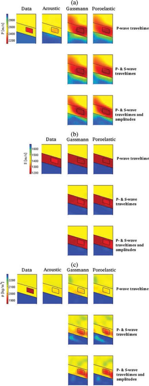
The model used to generate the poroelastic data is listed under the heading ‘Data’, and inverted models based on acoustic, Gassmann elastic and poroleastic modelling are listed under the headings ‘Acoustic’, ‘Gassmann’ and ‘Poroelastic’, respectively. The rows correspond to inversions based on direct P-wave traveltimes anomalies, direct P- and S-wave traveltime anomalies and direct P- and S-wave traveltime and amplitude anomalies, as indicated. (a) Compressional wave speed. (b) Shear wave speed. (c) Bulk density.

Open in new tabDownload slide

Figure 6

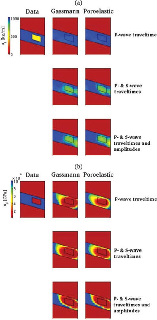
The model used to generate the poroelastic data is listed under the heading ‘Data’, and inverted models based on Gassmann and poroleastic modelling are listed under the headings ‘Gassmann’ and ‘Poroelastic’, respectively. The rows correspond to inversions based on direct P-wave traveltime anomalies, direct P- and S-wave traveltime anomalies and direct P- and S-wave traveltime and amplitude anomalies, as indicated. (a) Fluid density. (b) Fluid bulk modulus. Note the saturated colourscale at 1 GPa to better appreciate the transition between recovered CO₂ and brine fluid bulk modulus values.

Open in new tabDownload slide

As illustrated in Fig. 5(b), the S wave speed anomaly induced by CO₂ injection is relatively weak. As expected, P-wave traveltime data alone cannot recover the induced anomaly, but the inclusion of S-wave data leads to reasonably good images based on all three theories.

The recovery of bulk density, illustrated in Fig. 5(c), is poor when based on just P-wave traveltime data, but improves considerably when S-wave traveltime data are included, and even further when both amplitudes and traveltimes are used.

Fluid properties, can only be determined for the Gassmann elastic and poroelastic cases, using relationships (1) and (12), respectively. Fig. 6(a) illustrates that P waves cannot constrain fluid density, but P and S waves together can be used to recover this parameter, in particular in the poroelastic case with amplitude constraints. Recovery of the fluid bulk modulus is challenging, as illustrated in Fig. 6(b). All data sets and modelling approaches have difficulty recovering both the amplitude and the spatial distribution of this parameter,

In general, the recovered amplitudes in Figs 5 and 6 are accurate, however the spatial resolution remains relatively poor even when using both traveltime and amplitude anomalies. This is due to the coverage of our synthetic experiment involving only four sources and 20 receivers compared to real surveys, which usually deploy hundreds of sources and receivers.

4.2 Misfit analysis

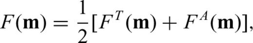
To assess the quality of the results based on the different theories (acoustic, Gassmann elastic and poroelastic) and three data sets (P-wave traveltimes, P- and S-wave traveltimes and P- and S-wave traveltimes and amplitudes), we investigate the reduction in the traveltime misfit function as a function of iteration number, as illustrated in Fig. 7. The flattening of all misfit functions at iterations three and four justifies termination of the inversion at that stage. The Gassmann elastic and poroelastic reductions in misfit are nearly indistinguishable. Note how traveltime inversion also helps to recover the amplitude of the signal, at least for the Gassmann elastic and poroelastic cases. The acoustic case shows no major improvement in amplitude fit, as already observed in Fig. 5. Finally, note how adding amplitude measurements does not drastically improve our results.

Figure 7

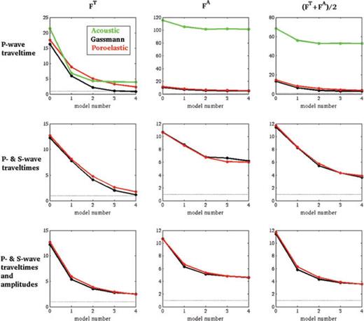
Evolution of the traveltime misfit, F^T, the amplitude misfit, F^A and the total misfit, F= (F^T+F^A)/2, as a function of iteration number; iteration 0 corresponds to the starting models, and iteration four to the final models. The rows correspond to inversions based on direct P-wave traveltimes anomalies, direct P- and S-wave traveltime anomalies and direct P- and S-wave traveltime and amplitude anomalies, as indicated. The dotted line identifies a misfit of one.

Open in new tabDownload slide

An alternative assessment of the quality of a model may be based on the logarithmic waveform variance reduction (‘waveform VRL’), which we introduce next. For a given set of model parameters m and a given arrival, we define a positive-definite non-dimensional measure of the waveform misfit by

13

where w_i(t) denotes a time window containing the arrival of interest, d(t) the data time-series and s(t; m) the corresponding synthetic seismogram for model m. Let S denote the number of sources and N_s the number of measurement windows associated with source s. The overall waveform misfit is defined by

14

A value of 0 ≤F(m) < 1 indicates that model m improves the fit of synthetics to data, and when F= 0 the synthetics fit the data perfectly. The corresponding waveform VRL is defined by (Tape et al. 2010)

15

where m₀₀ denotes the starting model and m_final the final model. As discussed in Tape et al. (2010), contrary to the usual variance reduction, the logarithmic variance is approximately Gaussian, which facilitates a more accurate definition of the mean value of the overall variance reduction. Values of VRL greater than zero indicate an improvement in fit.

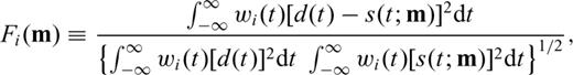
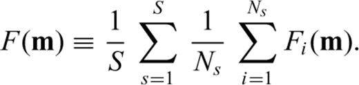
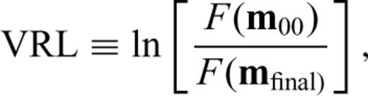
Fig. 8 shows the waveform misfit (14) and VRL (15) for the different theories and three data sets, which facilitates quantification of how various combinations of P- and S-wave traveltime and amplitude anomalies affect waveform fits. Improvement of the updated model with respect to the initial model translates into a migration of the waveform misfit (14) towards zero along the x-axis, and a migration of the VRL towards more positive x values. Both measures of misfit show improvements in fit when additional data are included in the inversion. Including S-wave data significantly improves the waveform fits, but the improvement in fit when P- and S-wave amplitude measurements are added to the traveltime measurements is marginal, as previously noted.

Figure 8

Waveform misfit analysis. The left column shows the behaviour of the waveform misfit (14) as a function of iteration number, and the right column shown the behaviour of the waveform variance reduction (Waveform VRL) (15). Values of VRL greater than zero indicate an improvement in fit. The three rows correspond to using acoustic, Gassmann elastic and poroelastic simulations, respectively. We clearly see the benefits of including both P- and S-wave traveltime data, and the limited impact of adding amplitude constraints.

Open in new tabDownload slide

5 Discussion and Conclusions

We have demonstrated that there is a poroelastic signature in time-lapse migration data collected for CO₂ sequestration monitoring, and that this signature cannot be captured using acoustic or elastic (with or without Gassmann's formulae) models. Using various combinations of direct P- and S-wave traveltime and amplitude anomalies, we have performed acoustic, Gassmann elastic and poroelastic time-lapse crosswell imaging and modelling of CO₂ injected into a porous aquifer. Inversions based solely on P-wave traveltimes constrain the bulk modulus in the acoustic case, the saturated bulk modulus in the Gassmann elastic case, and the B Biot modulus in the poroelastic case, because these moduli define the fast compressional wave speed. There is not enough P-wave information to constrain bulk density, shear wave speed and fluid density. Bulk density and shear wave speed (plus fluid density when using Gassmann elastic and poroelastic rheologies) are all correctly recovered using combined P- and S-wave information. We note improved spatial resolution of the (fast) compressional wave speed and the fluid bulk modulus when using both traveltime and amplitude anomalies. A major advantage of using the full poroelastic theory is the ability to constrain the fluid bulk modulus and the fluid density. Similar to bulk density, fluid density is only resolved if both P- and S-waves are used.

It is important to realize that in the isotropic poroelastic case there are a total of eight characteristic parameters (namely, ) for which sensitivity kernels may be defined (Morency et al. 2009). In this study, we chose to focus on three of them: and . Kernels associated with these three parameters are calculated based on the interaction of forward and adjoint solid displacements. The remaining five kernels involve the interaction of forward and adjoint relative fluid displacements or a combination of forward and adjoint solid and relative fluid displacements. As discussed in Morency et al. (2009), seismographic recordings of the solid displacement cannot accurately constrain parameters whose kernels are dependent on relative fluid displacement. A direct measure of relative fluid displacement could fill this gap. To that end, it would be interesting to investigate electrokinetic effects associated with pore fluid flow (Frenkel 1944; Pride & Morgan 1991), which may induce measurable electric signals (Ivanov 1939; Martner & Sparks 1959) and provide a direct measure of relative fluid displacement. Recently, Jardani et al. (2010) discuss a stochastic joint inversion of seismic and seismoelectric signals data. A synthetic seismic reflection case study representing a buried reservoir illustrates the recovery of most of the material properties with good precision, highlighting the potential of coupled seismic and electromagnetic wave propagation.

In the future, we plan to investigate joint crosswell seismic and electromagnetic data to better constrain fluid properties, such as permeability and porosity, through other poroelastic sensitivity kernels. Our plan is to take advantage of full waveforms using the FLEXWIN software developed by Maggi et al. (2009), which facilitates automatic measurement window selection.

Acknowledgments

The numerical simulations presented in this paper were performed on computational resources supported by the PICSciE-OIT High-Performance Computing Center and Visualization Laboratory (Princeton University). The authors thank Editor-in-Chief Jeannot Trampert, Louis De Barros and an anonymous reviewer for providing pertinent comments, which helped improve the manuscript, and Carl Tape for critical discussions on inversion procedures. This research was supported in part by a grant from Total.

Appendix

Appendix A: Governing Equations

In this section, we briefly summarize the governing equations for acoustic, elastic and poroelastic wave propagation.

A1 Acoustic wave equation

Wave propagation in an inviscid fluid is governed by the scalar wave equation (Chaljub & Valette 2004; Komatitsch et al. 2005)

(A1)

where the acoustic fluid displacement, u_a, is given in terms of the scalar potential, χ_a, by u_a=ρ⁻¹_a∇χ_a, whereas the acoustic pressure p_a is given by p_a=−∂²_tχ_a. The acoustic density is ρ_a, and κ_a denotes the acoustic bulk modulus.

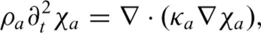
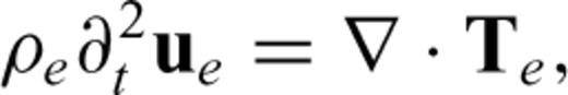
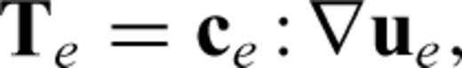
A2 Elastic wave equation

The equation of motion for an elastic medium is

(A2)

where u_e denotes the elastic displacement and ρ_e the elastic density. The elastic stress is determined by

(A3)

where c_e is the fourth-order elastic tensor. For an isotropic material we have

(A4)

where κ_e and μ_e denote the elastic bulk and shear moduli, respectively.

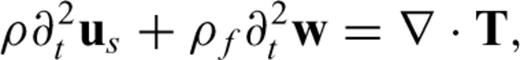
A3 Poroelastic wave equation

The governing equations for poroelastic waves are based on Biot's theory expressed in terms of the solid displacement u_s and the relative fluid displacement w=ϕ(u_f−u_s) (Biot 1956a,b; Carcione 2007; Morency & Tromp 2008)

(A5)

(A6)

Here ρ denotes bulk density, ρ_f fluid density, ϕ porosity, η_f fluid viscosity, k permeability and m=ρ_fc/ϕ, where c is the tortuosity. The constitutive relationships for an isotropic poroelastic medium are

(A7)

for the total stress and

(A8)

for the fluid stress. The identity tensor is denoted by I, and D_s is the solid strain deviator

(A9)

where a superscript T denotes the transpose. The macroscopic moduli B, C and M correspond to the Biot coefficients—defined in terms of the frame, solid grain and fluid moduli—while μ_fr denotes the frame shear modulus (Geertsma & Smit 1961; Stoll & Bryan 1970).

References