Time variations of aftershock decay parameters of the 2009 April 6 L'Aquila (central Italy) earthquake: evidence of the emergence of a negative exponential regime superimposed to the power law

Summary

1 Introduction

The L'Aquila earthquake of 2009 April 6 was the most deadly and destructive seismic event occurred in Italy since the big Irpinia earthquake of 1980 November 23. More than 300 people were killed and a significant portion of dwellings was severely damaged (maximum Mercalli intensity IX-X) within the town (counting about 70 000 inhabitants) and in its surroundings. The M_w= 6.3 main shock originated from a normal fault striking 134° SE and dipping 56° SW that extends 15–18 km along strike and 8 km along dip (Chiarabba et al. 2009; Pondrelli et al. 2010).

The study of the aftershock sequence of this earthquake is particularly significant because this is the strongest seismic event occurred after the reorganization of the Italian National Seismic Network (INSN) that, starting from 2005 April 16, improved much the detection capability and the homogeneity of magnitude determination over the whole Italian territory (Amato & Mele 2008). During the first seven months after the main shock, several thousands of aftershocks were located by the INSN that presently counts more than 230 stations (mostly equipped with three component seismometers) managed by the Istituto Nazionale di Geofisica e Vulcanologia (INGV) and by other observatories in Italy and in surrounding countries.

Only two aftershocks (occurred few days after the main shock, on April 7 and 9) had a magnitude within a unit or less of the main shock (M_w= 5.6 and M_w= 5.4, respectively). As INSN calculate only Ml magnitude (from synthetic Wood-Anderson waveforms) for most of the shocks, we will refer now on to such magnitude that in Italy slightly underestimates M_w (estimated Ml are 5.8 for the main shocks and 5.3 and 5.1, respectively for the two largest aftershocks).

The evolution with time of the aftershocks rate after a main shock is usually modelled by the power law that Omori (1894) found to describe well the decay of the 1891 Nobi (Japan) earthquake sequence, in the modified form proposed by Utsu (1961). The Omori's model is empirical in nature but it is hypothesized (Dieterich 1994) that aftershocks and other forms of earthquake clustering arise from stress perturbations of previous earthquakes that change the subsequent rate of earthquake activity. According to such theory, the aftershock rate would follow a decay equation that under certain conditions coincides with the Omori's law.

The Omori–Utsu law was applied successfully in different areas of the world to reproduce sequence decay and to predict aftershock probabilities (e.g. Reasenberg & Jones 1989; Eberhart-Phillips 1998; Lolli & Gasperini 2003). However, some recent works (Narteau et al. 2003; Gasperini & Lolli 2009) showed that, for many sequences, a faster exponential decay emerges from some weeks to some months after the main shock. According to the results of slider-block simulations by Narteau et al. (2003), this faster regime would be related to the complexity (or roughness) of the fault geometry, the higher the complexity the earlier the emergence of the exponential decay. However other physical mechanisms might be advocated (Ben-Zion & Lyakhovsky 2006; Klein & Wright 2008).

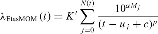
All previous decay models describe the (primary) triggering of aftershocks as the effect only of the stress perturbation associated with the main shock, neglecting the possible (secondary) triggering by the aftershocks. When applied to real sequences, such simple models are usually able to describe well the decay if the largest aftershocks are definitely weaker than the main shock (e.g. a magnitude unit less). When instead the sequence is characterized by several strong shocks having similar magnitudes, like for example the sequence occurred in 1997–1998 in Umbria–Marche (Amato et al. 1998; Deschamps et al. 2000) at about 80 km of distance from L'Aquila, such models clearly fails to reproduce the aftershock rate increases that usually occur just after each strong aftershock. According to the hypothesis that any aftershock induces a stress perturbation that may affect the rate of subsequent aftershocks, Ogata (1988) proposed the epidemic type aftershock sequence (Etas) model, in which all of the shocks of the sequence contribute to the predicted rate as a function of their respective magnitude.

Marzocchi and Lombardi (2009) employed the Etas model to producing real-time daily forecast of the spatio-temporal evolution of the L'Aquila sequence that have been provided to the Italian Civil Protection for managing the emergency. The real-time spatio-temporal forecasting of aftershock sequences is also performed routinely in California by the STEP group (Gerstenberger et al. 2005) using a non-epidemic model. On the other hand, Hainzl et al. (2008) demonstrated that Etas modelling of a space-dependent point-process might overestimate the forecasted rate due to the assumption of anisotropic clustering in space.

In our analysis, which resembles somehow the real-time computations we made almost each week during the first months after the main shock, we neglected the spatial aspects and focused on the time evolution of the aftershock rate that, in the first two months, showed unusual properties as a particularly slow decay in the first weeks that was followed by a progressive acceleration as well as a scarce sensitivity to the occurrence of strong aftershocks. We also considered a renewal of the aftershock rate within the main fault area that took place, about 80 days (d) after the April 6 main shock, just before and after the activation of a previously silent fault segment located at more than 25 km from main shock.

2 Data

We preliminary considered the shocks with Ml ≥ 2.3 detected by the INSN (downloaded from web site http://iside.rm.ingv.it) since main shock and up to 2009 November 4, within a radius of 50 km (blue circle in Fig. 1a and b) from the main shock epicentre (Lat = 42.334°, Lon = 13.334°). The main shock and the strongest aftershocks are evidenced in Fig. 1 by larger coloured dots. The lower magnitude limit (main shock magnitude minus 3.5), well above the completeness threshold in quiet periods (around Ml = 1.7 according to Amato & Mele 2008), is chosen so that to mitigate catalogue incompleteness in the first times after the main shock (Gasperini & Lolli 2009).

Figure 1

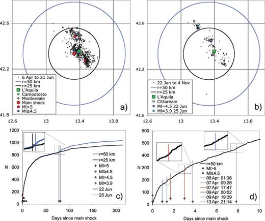
Spatial distribution of L'Aquila aftershocks before (a) and after (b) 2009 June 22. Coloured dots indicate the epicentres of main shock and of strongest aftershocks. (c) Cumulative number of aftershocks over the entire time interval from the main shock to 2009 November 4, within a radius of 50 km (blue line) and of 25 km (black) from main shock epicentre. Diamonds indicate the times of occurrence of strongest aftershocks. The inset shows that a sudden increase of the aftershock rate occurred in both areas on 2009 June 22. (d) Cumulative number of aftershocks in the first 10 d after the main shock. Insets show that in two cases an increase of the aftershock rate has occurred few hours before a strong shock, rather than just after it. A grey circle highlights the only strong aftershock (occurred on 2009 April 7, at 9:26) that appears to have produced an appreciable increase of aftershock rate.

Open in new tabDownload slide

The spatial distribution of aftershock epicentres within a radius of 25 km from the main shock (black circles in Fig. 1a and b) covers quite uniformly the surface projection of the two main fault segments that have been active since the first days after main shock: the southeastern one, located close to the city of L'Aquila, activated just after the April 6 main shock, and the northwestern one, located close to the small towns of Campotosto and Montereale, activated completely few days later (see fig. 1b of Chiarabba et al. 2009). We focused our analysis on the seismic activity of this area that it is well separated spatially and temporally from surrounding activity and namely from the narrow cluster of shocks located at longer distance on NW (close to the small town of Cittareale), with maximum Ml = 3.9 occurred on June 25 (light blue dot in Fig. 1b), corresponding to the activation of a fault segment that was almost silent up to about 80 d after the main shock.

From both Fig. 1(a) and (b) we can infer visually that the background seismicity with Ml ≥ 2.3 has been rather low in the surrounding areas during the entire time interval. Moreover, Marzocchi and Lombardi (2009) estimated a background rate of 0.18 shocks d⁻¹ for Ml > 1.5 in the 4 yr preceding the main shock, over a larger area (one degree wide in latitude and longitude). We can deduce that background activity for our magnitude threshold (Ml > 2.3) and our area of interest (within 25 km from main shock) was at least one order of magnitude lower (less than one shock per month). As the rate never decreased below one shock per week, over the entire time interval considered, we confidently neglected the background activity in our analyses.

The cumulative plot of the number of shocks with time elapsed since the main shock (Fig. 1c) shows that on June 22 the aftershock rate increased clearly within the widest radius (blue circle) and slightly even within the narrowest one (black circle). Even if the largest shock of the sequence in the NW with Ml = 3.9 (light blue diamond) occurred only three days later, the onset of the rate increase appears to be almost coincident with the occurrence on June 22 of a strong aftershock with Ml = 4.5 (blue diamond) located in the main fault area (blue dot in Fig. 1b).

Such an increase of the rate cannot be observed clearly after other strong aftershocks of the L'Aquila sequence. In fact, the shocks with Ml ≥ 4.5, all occurred in the first 10 d after main shock (Fig 1d), seem to have had negligible effects on the rate (excepting maybe that one, circled in Fig. 1d, occurred on April 7 at 09:26). Conversely two of the strongest aftershocks seem to be preceded rather than followed by slight increments of the rate (see insets in Fig. 1d). This poor correlation between rate increments and the occurrence of strong aftershocks is at odds with what occurred in 1997–1998 for the Umbria–Marche sequence when almost all of the strongest aftershocks were followed by a clear renewal of sequence activity, particularly in the first month after the main shock (Fig. 2).

Figure 2

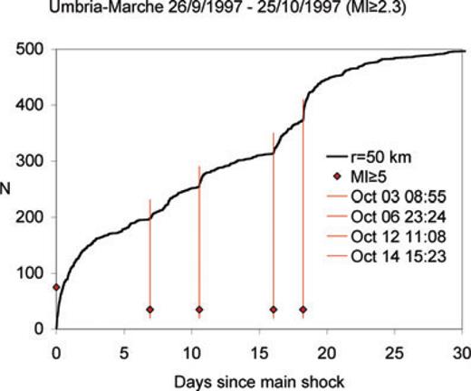
Cumulative number of aftershocks in the first 30 d after the 1997 September 26 Umbria–Marche main shock. Diamonds and vertical lines indicate the times of occurrence of strongest aftershocks. In all cases a sudden increase of the aftershocks rate occurred just after each strong aftershocks.

Open in new tabDownload slide

3 Likelihood Analysis

We modelled the time-series of aftershocks by maximizing the log-likelihood function of a Poisson process with variable rate (see Ogata 1988), according to the Modified Omori Model (MOM, Utsu 1961)

1

and the band Limited Power Law (LPL, Narteau et al. 2002, 2003)

2

where γ and Γ indicate the incomplete and the complete Gamma function, respectively. The formulation of eq. (2) slightly differs with respect to the original one by Narteau et al. (2002) that indicates q and A in place of p and K/Γ(p), respectively. We also considered a simple decay model consisting of the product of the MOM with a negative exponential that we will name Power-Law Exponential (PLE)

3

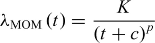
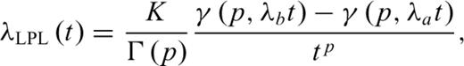
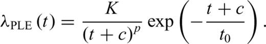
The meaning of parameters p is the same for all of the models (the power-law exponent). Parameter c, common to both MOM and PLE, represents a time delay before the onset of the power-law decay that is usually attributed to the incompleteness of the catalogue (e.g. Lolli & Gasperini 2006) or to peculiar decay regimes occurring in the first times after the main shock (Peng et al., 2006,2007). Lolli et al. (2009) showed that c corresponds to the time at which the rate deviates of a factor 2^{− p} from a Pure Power Law (PPL) at short times. Parameter t₀ of the PLE is the characteristic time of the exponential regime and corresponds to the time at which the rate deviates of a factor 1/e (base of natural logarithms) from a PPL at long times. Lolli et al. (2009) also defined two times t_b and t_a as a function of the LPL parameters λ_b and λ_a, having the same physical meaning of c and t₀, respectively, which can be useful to compare the LPL with other models. Finally, K represents, for all models, a normalizing term corresponding to the ratio between the total number of aftershocks and the integral of the time dependent part of the rate functions, so that the time integrals of the complete rate functions λ(t) from T_s to T_e equate the number of observed aftershocks.

The LPL and PLE models predict both three regimes of decay (Fig. 3): an initial phase in which the rate is nearly constant, then an intermediate one characterized by the power law, and a final one in which the negative exponential becomes dominant. In Fig. 3, we can also note that the PLE is almost coincident with the MOM at short times and with the LPL at long times.

Figure 3

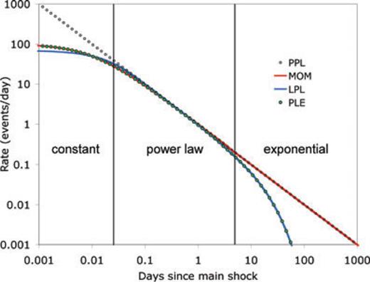
Theoretical aftershock rates for different decay models using the same set of parameter values (p = 1, c = t_b = 0.01 d, t₀= t_a = 20 d, K = 1). The MOM (red line) coincides with the PLE (green circles) at short times and converge to a pure power law (open circles) at long times. The PLE coincides with the LPL (blue line) at long times. All the models follow a power-law decay with p = 1 at intermediate times.

Open in new tabDownload slide

In principle any decay model can be implemented in epidemic form but in the case of the LPL this is particularly consuming in terms of computer time because each log-likelihood function evaluation requires a number of Gamma function computations that is about the square of the number of aftershocks in the sequence (see Appendix). For example, the fitting of the entire L'Aquila sequence (about 950 shocks) takes about seven hours, using a 2.2 GHz CPU. This makes such model not particularly suited for real-time modelling and forecasting of seismic sequences. The rate equations for the three models are

4

5

6

where u_j and M_j are respectively the time and the magnitude of the jth shock, N(t) is the total number of shock occurred up to time t (including main shock with j = 0), K′ is again a normalizing factor that depend on the total number of shocks and on the time integral of the sum and α is the coefficient of secondary aftershock productivity as a function of shock magnitude.

A debate is open in the literature on the physical meaning of α and on its relation with the b-value of the Gutenberg–Richter law. Some works (Console et al. 2003; Helmstetter 2003; Zhuang et al. 2004, 2005; Gasperini & Lolli 2006; Christophersen & Smith 2008) find values of α significantly lower than b, while others (Felzer et al. 2004; Marsan 2005; Helmstetter et al. 2005) supported the argument that α and b are both of the order of 1, and physically interpreted such evidence by arguing that both parameters are related to the fractal dimension of the spatial distribution of hypocentres (D ≈ 2), according to the relation α≈ b ≈ D/2.

The equality of α and b would imply that the contribution of small and large shocks to stress variations (and hence to the rate) is about the same because the frequency of small earthquakes almost exactly compensates their lower triggering potential (Marsan 2005). This, however, would imply that any statistical fitting of real sequences would be biased by the cut of the shocks below the magnitude completeness threshold. Obviously, this argument is somehow specious as empirical evidence, starting from the seminal work by Omori (1894), indicates that in most cases the decay of aftershocks can be reproduced well even considering only the effects of the strongest shocks or even of the strongest one.

The details on maximum likelihood estimation of parameters and of relevant formal confidence intervals for all of the decay models are reported in the appendix.

4 Results

In the following, we analyse the time decay of the L'Aquila main sequence (within 25 km from main shock) by considering time intervals of progressively increasing duration from 5 to 213 d. This mimics somehow the evolution with time elapsed from main shock of the results of real-time analyses that we have made actually while the sequence was still ongoing and the data set included the shocks located and sized by the INSN up to that moment.

4.1 Non-epidemic models

In Fig. 4(a) we can see that, in the first days after main shock, the estimated power-law exponent p for the MOM (red), the LPL (blue) and the PLE (green) models, was definitely smaller (p = 0.3–0.6) than previous average estimates made by Lolli & Gasperini (2003), using the MOM, for the entire Italian area (p = 0.93, thick black line) and for two close areas of Val Comino (p = 1.09, thin black) and Marche (p = 0.95, dashed black) located at distance of about 80–100 km from L'Aquila on SSE and on NNW, respectively. Starting from durations of 15 d, the p-value of the MOM begins to increase up to reach values well above 1 for durations longer than 60 d. Conversely, for durations shorter than 60 d, the LPL and the PLE show rather stable p values (well within 1-σ error bounds) around 0.35 and 0.45, respectively. For durations longer than 60 d, p starts to increase even for such models up to reach values of about 0.6 for the LPL and 0.8 for the PLE for durations of 110 d and longer.

Figure 4

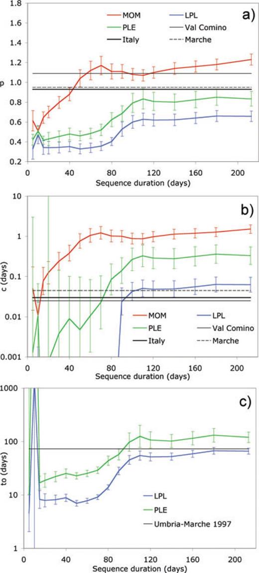
Variation with sequence duration after main shock of the power-law exponent p (a), of the time delay of the onset of the power-law c (b) and of the characteristic time of exponential regime t₀ (c) for non-epidemic models. Black horizontal lines in (a) and (b) indicate average values computed, using the MOM, by Lolli & Gasperini (2003) for the whole Italy (solid thick) and for two neighbouring areas of Val Comino (solid thin) and Marche (dashed). The black horizontal line in (c) indicates the t₀ value computed, using the LPL, by Gasperini & Lolli (2009) for the 1997–1998 Umbria–Marche sequence. Error bars indicate 68 per cent confidence intervals computed by formal methods for p, log c and log t₀ (see appendix).

Open in new tabDownload slide

By comparing Fig. 4(a) and (b), we can note that the behaviour of the time delay of power-law onset c of the MOM is strictly correlated (positively) with the power-law exponent p. For durations longer than 60 d, c reaches values close to 1 d that cannot be justified by the usual arguments of the incompleteness of the catalogue (e.g. Lolli et al. 2009) or of different decay regimes occurring in the first times after main shock (Peng et al. 2006, 2007) because these, in case, should be more effective in the first days after the main shock rather than at long times. A certain amount of correlation between p and c can also be noted for the PLE but, for durations shorter than 60 d, the variations of the two parameters lie within the error bounds. For the LPL, the parameter t_b (equivalent to c, according to Lolli et al. 2009) is virtually zero for durations shorter than 90 d and then increases suddenly to about 0.05 d for longer time durations. We must note that very small c values, below say 0.01–0.001 d, indicate that the rate decay differs significantly from a PPL only in the first hours after main-shock. Hence, even large relative variations of c below such limits do not affect the likelihood function very much and this is reflected by very large error bounds (Fig. 4b).

A significant positive correlation between parameters p and c of the MOM has been evidenced already by Gasperini & Lolli (2006) for sequences of Italy and California. More recently, Lolli et al. (2009) and Gasperini & Lolli (2009) argued, on the basis of the analysis of simulated and real sequences respectively, that such correlation might be the symptom of the emergence of an exponential regime of decay that is controlled by the characteristic times t₀ for the PLE and t_a for the LPL.

The behaviour of t₀ and t_a as a function of sequence duration is plotted in Fig. 4(c) where we can see that, after some oscillations in the first 10 d, they stabilizes to values of about 15–20 d for the PLE and 8–10 d for the LPL that remain quite constant up to durations of 60–70 d. For longer durations, t₀ and t_a begin to increase up to reach values of about 100 and 50 d, respectively. The relatively narrow confidence intervals indicate that characteristic times are quite well constrained by the data for both models. Furthermore, we can note that their values in the first 60 d are definitely lower than those computed by Gasperini & Lolli (2009) using the LPL model (73 d), for the 1997–1998 Umbria–Marche sequence, while they become of the same order of magnitude at longer durations.

The better performance of LPL and PLE with respect to MOM can be tested statistically by the corrected Akaike Information Criterion (AICc, Akaike 1974, Hurvich & Tsai 1989). In Fig. 5, we show the plot of the differences between the AICc scores of the different models and that of the MOM. Such scores are computed according to Lolli et al. (2009) so that the most preferable model is that one with the largest positive difference. The MOM has to be preferred with respect to the LPL and the PLE only for durations shorter than 10 d. For longer durations up to about 60 d, we can note a clear increase of the ΔAIC_c scores for both the LPL and PLE, then they remain about constant up to 80 d, when the trend inverts up to reach scores similar to the MOM for duration of 110 d, when the trend inverts again. The scores of the LPL and the PLE are very similar to each other for all of the durations, with a slight prevalence of the LPL from 60 to 100 d and of the PLE for durations longer than 100 d. These results clearly indicate that the standard MOM does not describe at best the aftershock decay of the L'Aquila sequence in the first 60 d and that a faster exponential decay emerges, starting from about 10–15 d after the main shock.

Figure 5

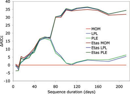
Variation with sequence duration after main shock of the differences between the AICc scores of the various decay models and that of the MOM, for the L'Aquila sequence. The preferred model is the one with largest positive AICc difference, according to Lolli et al. (2009) formulation.

Open in new tabDownload slide

The better fit in the first 60 d of the LPL and PLE models with respect to the MOM can be visualized by the plot of the residuals of the cumulative number of shocks as a function of the number of shocks (Fig. 6a) and of the time elapsed after the main shock (Fig. 6b). We can note that the cumulative number of shocks predicted by the LPL and the PLE (light blue and light green lines) differ from the observed one (black zero line) by less than 20 shock over the entire time interval and are particularly accurate after day 20 when the exponential decay became dominant. Conversely the MOM (light red) overestimates the number of shock up to about 35–40 shocks, from day 2 to day 9, and underestimates up to about 25 shocks, from day 9 to day 60.

Figure 6

Differences between the observed cumulative number of shocks and those predicted by various decay models as a function of the number of shocks (a) and of the time elapsed after the main shock (b). Model parameters are estimated by considering all (Ml ≥ 2.3) aftershocks occurred in the first 60 d after the main shock. Red and blue diamonds indicate the occurrence of strong shocks with Ml > 5 and Ml ≥ 4.5, respectively.

Open in new tabDownload slide

The response of the MOM parameters to the emerging exponential decay can be explained geometrically as follows: as the log–log plot of the rate at long times is not actually a straight line but rather a curve with downwards concavity (see LPL and LPL plots in Fig. 3), the p-value (corresponding to the average slope of the curve with the sign changed) increases progressively as the deviation of the curve from the straight line becomes more effective with increasing durations. As well the c-value also progressively increases to compensate the deviation a short times due to the increased p-value and this brings to the observed correlated increase of both p and c as a function of the considered time duration of the sequence.

We could also argue that a further change of the properties of the sequence took place after 60 d, a couple of weeks before the activation, around day 80, of a previously silent fault section in the NW (Fig. 1b). Even if the data of such subsequence are excluded from previous analysis and are quite well separated spatially from the main fault system activity, we might hypothesize the existence of some form of interaction between the two fault sections.

4.2 Epidemic models

An alternative description of the evolution of the L'Aquila sequence may be given in terms of epidemic processes. The evolution with sequence duration of p estimated by epidemic models (Fig. 7a) appears rather variable for durations up to 40–50 d, when the majority of the shocks did occur. For Etas MOM (dark red line) and Etas LPL (dark blue), p oscillates in the range 0.6–1.3 while for Etas PLE (dark green) it decreases almost monotonically from about 1.7 to about 1.0. For longer durations, p stabilizes to about 1.2 for Etas MOM (similar to non-epidemic MOM) and to about 1.0 for Etas LPL and Etas PLE (significantly higher than non-epidemic counterparts in Fig. 4a). Conversely the estimated c (Fig. 7b) remains rather stable within the range 0.05–0.20 d for all models. For long durations the c-value for Etas MOM and Etas PLE is significantly lower than the estimate made by the corresponding non-epidemic models (Fig. 4b), while for Etas LPL it is very close to the non-epidemic LPL.

Figure 7

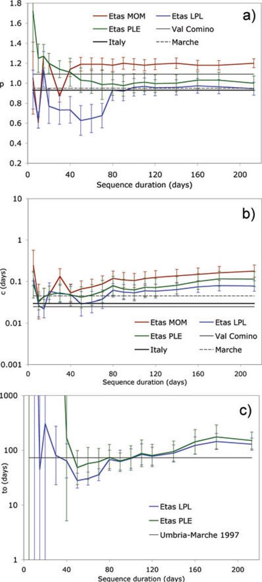
Same as Fig. 4 but for Etas MOM, Etas LPL and Etas PLE models.

Open in new tabDownload slide

The behaviour of the characteristic times of exponential decay (t₀ for the Etas PLE and t_a for the Etas LPL, dark green and dark blue lines respectively in Fig. 7c) differs significantly from those of the non-epidemic models for duration shorter than 40 d when they are larger than 100 d for Etas LPL and virtually infinite for Etas PLE. For longer durations the estimated t₀ and t_a for the two models tend to converge to each other and substantially coincide for durations longer than 80 d when they assume values around 100 d that are similar to non-epidemic PLE and are slightly larger than non-epidemic LPL.

In Fig. 5, we can see that, for durations shorter than 80 d, Etas MOM (dark red), Etas LPL (dark blue) and Etas PLE (dark green) give AICc scores very similar to non-epidemic LPL (light blue) and PLE (light green) while epidemic models overperform clearly non-epidemic ones for longer durations. This behaviour differs markedly from that observed for the 1997–1998 Umbria–Marche sequence (Fig. 8), for which AICc differences indicates a clear preference for the epidemic models since the first days after the main shock. From the plot of the differences between observed and predicted cumulative numbers of shocks in the first 60 d (Fig. 6), we can note that Etas MOM (dark red line) and Etas PLE (dark green) models deviate from observation more than non-epidemic LPL and PLE at times shorter than about 4 d and slightly less between 10 and 15 d, while the performances are similar between 4 and 10 d. The Etas LPL is similar to non-epidemic LPL and PLE for times shorter than 4 d, is worse between 4 and 10 d and better between 10 and 15 d. Between 15 and 60 d, the Etas PLE and Etas LPL are definitely more accurate than Etas MOM but non-epidemic LPL and PLE models are even more accurate.

Figure 8

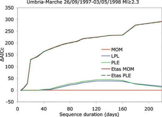
Same as Fig. 5 but for the 1997–1998 Umbria–Marche sequence. Epidemic models overperform clearly non-epidemic ones since 10 d after main shock.

Open in new tabDownload slide

The definitely higher AICc scores for durations longer than 80–90 d suggest that epidemic models describe the entire L'Aquila sequence comprehensively better than non-epidemic ones. However, the marked instability of epidemic parameters at times shorter than 40–50 d and the equivalence of epidemic AICc scores with non-epidemic LPL and PLE in the first 60–80 d indicate that before June 22 the epidemic character of the L'Aquila sequence is very weak and that models of primary triggering that include an exponential acceleration of the power-law decay might best describe the aftershock generation process.

A further confirmation comes from the behaviour of the coefficients of secondary productivity α (Fig. 9). For the Etas MOM (dark red) we can see large oscillations for durations shorter than 40 d that are a symptom of poor constraint by the data. For longer durations α stabilizes to values that are significantly lower than the b-value up to about 80 d and became larger for durations longer than 160 d. For the Etas LPL (dark blue) the α-value is unrealistically high (about 1.5) and poorly constrained (large error bars) up to durations of 80 d when it stabilizes to values close to 1. For the Etas PLE (dark green), the α-value shows a clear increasing trend up to durations of 80 d but remains well below the b-value up to durations of about 60–70 d. Considering that the (1-σ) error bars do not overlap, we can assert confidently that in the first part of the sequence Etas PLE α is significantly lower than b, while the two parameters substantially coincide for longer durations.

Figure 9

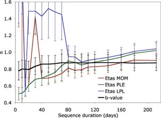
Variation of the coefficient of secondary productivity α of epidemic decay models and of Gutenberg–Richter slope (b-value) with sequence duration after the main shock. Error bars indicate 68% confidence intervals computed for α by formal methods.

Open in new tabDownload slide

More in general, such results confirms that epidemic models are poorly constrained by the data for durations shorter than 60–80 d and that only for longer durations the sequence assumes a clear epidemic character. For durations longer that 80 d the estimated α for all epidemic models shows a slightly increasing trend but does not differ significantly from the b-value. In the case of Etas PLE, the almost monotonic increasing trend of α resembles somehow a similar trend of the b-value thus suggesting that the two parameters might be correlated somehow.

4.3 Magnitude independent productivity

Reasenberg & Jones (1989) assumed that the normalizing term K of the MOM is a function of the minimum magnitude threshold (M_c), of the main shock magnitude (M_m) and of the b-value of the Gutenberg–Richter law as

7

where a would represent an index of the overall productivity of the sequence, independent of the magnitude. We could argue that such definition is somehow biased by the actual values of MOM parameters p and c as K depends also on the integral of the time dependent part of the rate function (see appendix). Felzer et al. (2004) and Christophersen & Smith (2008) proposed unbiased definitions of sequence productivity but we adopt here eq. (7) for comparison with the estimates made for Italy by Lolli & Gasperini (2003) using the Reasenberg & Jones (1989) formulation.

We can see in Fig. 10 how the productivity a is one unit above (a factor of 10 in terms of the number of triggered shocks) to those computed by Lolli & Gasperini (2003) for the whole Italian area (a =−1.66) and for the Marche area (a =−1.63) and even a half of a unit above (a factor of about three in terms of the number of shocks) to that computed for the Val Comino area (a =−1.15), which is the most productive area of Italy according to such authors.

Figure 10

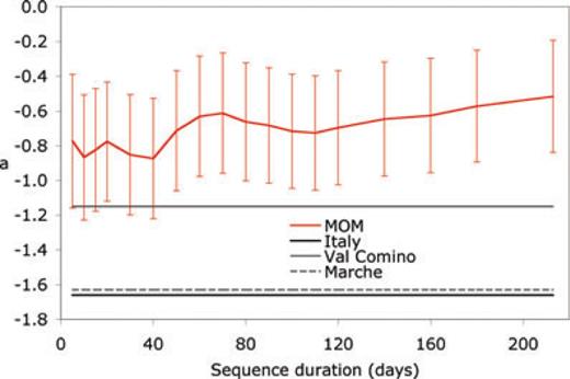
Variation of main shock productivity a of the Reasenberg & Jones (1989) model with sequence duration after the main shock. Horizontal lines indicate average a-values computed for whole Italy (solid thick) and for two neighbouring regions of Val Comino (solid thin) and Umbria Marche (dashed) by Lolli & Gasperini (2003). Error bars indicate 68% confidence intervals computed for a by formal methods.

Open in new tabDownload slide

We could hypothesize that the a-value computed for the L'Aquila sequence might be possibly biased high due to an underestimation of main shock Ml magnitude as the M_w– Ml difference for the main shock (0.5) is larger than for the strongest aftershocks (0.3). For example, by assuming that the correct Ml of main shock is 6.0 instead of 5.8, the productivity a would reduce of about b × 0.2 = 0.17 units, thus becoming very close to previous estimates made for Val Comino but still remaining far from the Italian and Marche averages. Assuming the typical Italian productivity (a =–1.66), the L'Aquila Ml magnitude should be about one unit larger than 5.8, to produce the same number of aftershocks.

5 Conclusions

Our analysis indicates that, in the first two months after the April 6 main shock, the L'Aquila aftershock sequence is described well by models of primary triggering but the MOM does not capture as well the time evolution of the aftershock rate. In fact, the higher AICc scores of the LPL model (Narteau et al. 2002, 2003) and of a simple model that combines a MOM with a negative exponential (PLE) indicate that a decay regime faster than power law clearly emerges starting from about 15 d after the main shock. For the MOM, which does not include such exponential term, this is reflected by the progressive and correlated increase of the power-law exponent p and of the time delay of power-law onset c.

The simple decay model we proposed here (PLE) showed to reproduce as well as the LPL the decay of the sequence but with a significant improvement in term of computational efficiency that allows to employing it routinely for real-time modelling and forecasting, even within an epidemic approach.

The magnitude independent productivity of the L'Aquila sequence is probably one of the highest ever-observed in Italy since the installation of a modern seismic network in mid 1980s. This agrees somehow with the high productivity observed by Lolli & Gasperini (2003) in the close area of Val Comino located at about 80 km of distance on SSE.

Different from the 1997–1998 Umbria–Marche sequence (occurred at about 80 km of distance on NNW), the rate of in the first two months after the main shock appears to be almost insensitive to the occurrence of strong aftershocks that in few cases seem to be preceded rather than followed by slight increases of the rate. The weak epidemic character of the sequence in this time interval is confirmed by the fact that epidemic models does not perform appreciably better than non-epidemic ones, according to the Akaike information criterion.

A progressive increase of the power-law exponent and of the characteristic time of the exponential decay for the LPL and PLE models took place starting from about a couple of weeks before the activation, around day 80, of a previously silent fault section in the NW at about 25 km of distance from main shock. We could argue that, albeit their spatial separation, there had been some interaction between the main fault system and the fault section in the NW and that the activation of the latter has been anticipated of some weeks by a slow change of decay properties of the main sequence. After such reactivation the Akaike scores become definitely better for epidemic models with respect to non-epidemic ones.

Our analysis, resembling somehow the real-time computations we performed actually when the sequence was still ongoing, indicates that the parameters of decay model might vary significantly with time during the occurrence of a sequence. Hence retrospective estimates of decay parameters using catalogue data of the entire sequence might not evidence such temporal variability of decay parameters.

In particular, the instability of model parameters with time may suggest that different physical processes other those that are usually considered in the literature might have a role in the process of aftershock generation. For example the correlated increase of MOM parameters p and c is a symptom of the emergence of a negative exponential decay, superseding the classic power law, which could be a consequence of a high complexity of the fault or of other physical mechanisms. As well, slow changes in the regime of decay, occurring even in absence of strong aftershocks and anticipating the activation of fault segments previously silent, might suggest the existence of interactions between well separated fault systems that, however, need to be verified by future analyses, considering also the spatial pattern of seismicity.

In fact, in our analysis we neglected the spatial variability of the seismicity pattern and the background (untriggered) seismic activity. While the background rate was confidently estimated being very low on the basis of empirical evidence, we cannot exclude that the validity of the achieved results might depend on the adopted approach to analyse only the temporal pattern.

Acknowledgments

We thank the anonymous referees and the Editor Massimo Cocco for their constructive criticisms and useful suggestions. This research has benefited from funding provided by the Italian Presidenza del Consiglio dei Ministri – Dipartimento della Protezione Civile (DPC). Scientific papers funded by DPC do not represent its official opinion and policies. One of the authors (B.L.) benefited from a 2 yr research grant founded by the Italian Ministero dell'Istruzione dell'Università e della Ricerca (MIUR) within the Project Airplane of the Istituto Nazionale di Geofisica e Vulcanologia.

Appendix

Appendix: Maximum Likelihood Estimation of Model Parameters

The likelihood function of a Poisson point process with variable rate λ is given by (see Ogata 1988)

(A1)

where T_s and T_e are the starting and ending times of the sequence and θ represents the parameter vector. Lolli et al. (2009) report the log-likelihood functions of the MOM and the LPL models in their appendix G. For the PLE model, defined in eq. (3) of main text, the log-likelihood function is given by

(A2)

where u_i and N are the occurrence times and the total number of aftershocks, respectively and I(p, c, t₀) is the time integral of the time dependent part of rate function from T_s to T_e. Such integral can be computed analytically for any p ≥ 0 in two forms: the first one holds for any non-integer p and the second one for any integer p

(A3)

where int indicates the highest integer that is lower than the argument, γ indicates the incomplete Gamma function, and E₁ indicates the Exponential Integral function 1 (Abramowitz & Stegun 1972).

As for the other models, the maximum-likelihood estimate of K for the PLE can be computed by equating to 0 the partial derivative of log-likelihood with respect to K

(A4)

that gives

(A5)

The likelihood functions of Etas MOM (4), Etas LPL (5) and Etas PLE (6) models can be derived from eqs. (A1), respectively as

(A6)

(A7)

(A8)

where B(t_j|p,c), F(t_j | p, λ_a, λ_b) and I(t_j|p, c, t₀) are the integrals of the MOM [see eq. (G3) in Lolli et al. 2009], of the LPL (eq. G9, ibidem) and of the PLE [eq. (A3) above] respectively, with the lower integration limit (T_s) replaced by 0 for any j ≠ 0 and the upper integration limit (T_e) replaced by T_e–u_j (u₀ is the occurrence time of the main shock). Note that the double sum in the second term of eq. 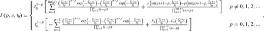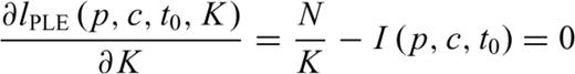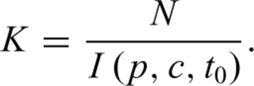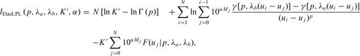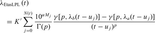(A7) implies the numerical evaluation of about Gamma functions. This explains why the Etas LPL model is so excessively time-consuming and hence it is not particularly suited for real-time modelling and forecast of seismic sequences.We maximized the log-likelihood function (for all models) by an algorithm, described by Lolli et al. (2009), that includes a random search and the refinement of the best random solutions. We computed formal 68 per cent confidence intervals (1-σ) by inverting the Hessian of the log-likelihood at the maximum and then taking the square roots of its diagonal elements (see for details Ogata 1988 and Lolli et al. 2009). To improve the speed and the accuracy of parameter determination, a logarithmic transformation is applied to c, t_b, t₀, t_b, K and K′ (see Lolli & Gasperini 2003). Hence, even the computed error bounds are logarithmically transformed. This is reflected by symmetric error bars in logarithmic plots of Figs 4(b) and (c), 7(b) and (c).

References