Inversion of first-arrival seismic traveltimes without rays, implemented on unstructured grids

Summary

1 Introduction

Seismic methods have the potential to provide much higher resolution than other geophysical techniques typically used in mineral exploration, namely gravity, magnetics, resistivity and electromagnetics. First-arrival seismic traveltimes can generally be reliably picked from seismic records and can be inverted to obtain possible distributions of the causative subsurface velocity.

Typical tomographic inversion algorithms make use of ray tracing in one or more ways. Bois et al. (1972) developed an algorithm in which curved rays are traced through a velocity medium to solve the forward problem to calculate first-arrival traveltimes. Many other authors advanced the approach within the same basic framework.

First-arrival ray tracing can be problematic when shadow zones exist or where multiple paths between source and receiver are possible (Vidale 1988). Where multiple paths exist, ray tracing provides no guarantee that a located path corresponds to a first or later arrival (Rawlinson et al. 2007). Due to the non-linear nature of the traveltime tomography problem, new rays must be traced every time the velocity model changes within the inversion algorithm and ray tracing can therefore become computationally impractical when many source–receiver pairs are considered. Although ray tracing on 2-D rectilinear grids is fairly trivial, extension to 3-D unstructured tetrahedral grids is more involved, requiring some significant implementation hurdles: see Sambridge & Rawlinson (2005) for a review of seismic tomography using irregular parameterizations.

Ray tracing can be avoided in the forward solution by calculating the first-arrival traveltimes with a finite-difference approach on a discretized domain. A thorough review of seismic ray tracing and wave front tracking via finite-difference approaches is provided by Rawlinson et al. (2007). Aldridge & Oldenburg (1993) developed an inversion approach that uses the finite-difference algorithm of Vidale (1988) in place of ray tracing for the forward solution. Rawlinson et al. (2006a,b) also used a finite-difference modelling approach in 3-D teleseismic tomography problems, employing the subspace inversion method of Kennett et al. (1988). Although those approaches avoid ray tracing in the forward solution, ray tracing is still used to calculate linearized sensitivity information relating changes in the model to changes in the data. These rays are back-traced from receiver to source following the steepest descent direction through the grid of computed traveltimes. This ray tracing carries less computational expense than the tracing replaced by the finite-difference forward solution but it still carries with it a fair amount of expense and implementation issues. Moreover, another issue with this approach is that the sensitivity calculation central to the inversion algorithm is not numerically consistent with the forward modelling solution employed, that is, the derivatives used are not the actual derivatives of the forward modelling equations but rather, as we show, can only be considered a rough approximation. The derivative information and the function being minimized in the inversion need to be numerically consistent with one another, otherwise the convergence of the minimization can be harmed.

We seek an approach for inverting first-arrival data that does not require ray tracing and involves a sensitivity calculation that is numerically consistent with a finite-difference forward solution. We forgo a full discussion of the details of our forward solution, much of which is provided in cited reference material. Instead, we focus on the details immediately relevant to the inverse problem. We then present our inversion approach, focusing on our method of calculating sensitivity information based on equations from the forward solution. Finally, we apply our inversion method to geologically realistic 2-D and 3-D synthetic examples based on real Earth scenarios. We compare our results against those from inversions that employ ray tracing.

Unstructured grids allow efficient generation of complicated subsurface geometries, such as those often encountered in hard-rock environments. This becomes important when one wishes to incorporate structurally complicated prior information into an inversion, which may be difficult or impossible to do adequately on a rectilinear grid. Also, unstructured grids can significantly reduce the problem size involved in forward and inverse calculations compared to rectilinear grids. It is for these reasons that we choose to work with unstructured grids, however, the inversion approach we develop is equally applicable to rectilinear grids. The derivations required for rectilinear grids will follow easily from those we provide for unstructured grids.

2 Solution of the Forward Problem

The material in this section is adapted from Lelièvre et al. (2011), to which we refer those readers wishing for a more detailed discussion and review of the relevant literature.

2.1 A summary of the Fast Marching method

Modelling of first-arrival seismic traveltimes via propagation of wave fronts is governed by the eikonal equation,

1

where t is traveltime and s is slowness (the inverse of velocity). Many authors have developed numerical methods for solving this equation on discretized domains. Each cell in the discrete grid is commonly assigned a constant slowness value, which is the approach taken here, but the slowness could also change within each cell following some simple function. The solutions begin by initializing the traveltimes at near-source grid nodes. Traveltimes at nodes neighbouring those are then calculated using finite-difference update formulae. The solution front continues to iterate outwards from the source until all grid nodes have been visited.

Vidale (1988) developed a solution for regular rectilinear 2-D grids in which the solution front marches away from a point source in a box shape. Many authors extended this work by maintaining the box-shaped marching but moving to rectilinear 3-D grids and improving modelling accuracy and stability. Others changed the marching scheme, including Sethian (1996) who developed an efficient ‘Fast Marching Method’ (FMM) that advances the solution front through the grid in a monotonic manner. The FMM solution fronts then mirror the seismic wave fronts. Box-style marching schemes rely on a rectilinear discretization, leaving the FMM as the method of choice for unstructured grids. Here we provide a brief overview of the algorithmic details of the FMM algorithm.

There are several methods for initializing the FMM solution. One choice is to assume that the slowness of the medium is homogeneous in the local vicinity of the point source. One can define an initialization radius and calculate the traveltime at each node within that radius by multiplication of the local homogeneous slowness by the distance from each node to the source. Initializing in this way can allow for a significant reduction in modelling error associated with the assumption of linear (in 2-D) or planar (in 3-D) wave fronts (that assumption is discussed further below). However, this strategy leads to an added complication in the inversion algorithm because it requires a homogeneous slowness around the source. We discuss this complication further in Section 3 but we can avoid it by simply discretizing more finely around the source, which also reduces the modelling error. In that case the initialization may calculate traveltimes only at the nodes directly surrounding the source, that is, the nodes that make up the cell containing the source. If the source lies directly on a grid node then no initialization is required beyond assigning that node a traveltime of zero.

Consider Fig. 1, which captures the FMM solution in part of a rectilinear grid at some later stage after initialization. Nodes can be categorized as being either ‘upwind’ or ‘downwind’ from the solution front. The downwind nodes are further categorized into a set of ‘close’ nodes immediately connected to upwind nodes, and a set of ‘far’ nodes not immediately connected to upwind nodes. Upwind nodes have firm traveltime values that can not be altered at later stages in the FMM solution. The traveltimes at the close downwind nodes are calculated based on the traveltimes at their neighbouring upwind nodes. Those calculations are referred to as local traveltime updates. For any particular close node, there may be several possible local update calculations. For example, for the circled close node in Fig. 1, the local update can be calculated through either of the two cells on its immediate left. The FMM calculates first arrivals so the actual traveltime taken by this node is the minimum of all those calculated through the local updates.

Figure 1

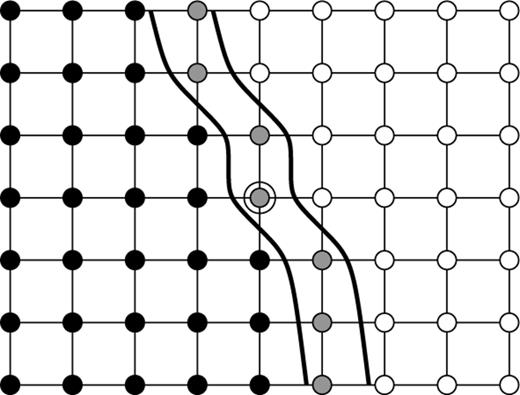
A section of a rectilinear 2-D grid through which an FMM solution is progressing. Grid nodes are represented as circles with thin connecting lines indicating the grid cells. Upwind nodes are filled black, downwind nodes that are ‘close’ are filled grey and downwind nodes that are ‘far’ are filled white. The central node is circled for referencing in the text. Two parallel thick lines represent either side of a narrow band of ‘close’ nodes.

Open in new tabDownload slide

Once all the local traveltime updates are calculated for the close nodes they define a narrow band of trial nodes that could be moved into the set of upwind nodes. The FMM moves the solution front forward monotonically to ensure causality is maintained. To do so, only the close node with the smallest traveltime is chosen to become an upwind node. Afterwards, any downwind nodes that were originally ‘far’ but are now connected to the new upwind node are added to the set of ‘close’ nodes. The procedure repeats until all nodes in the grid are upwind. The FMM is so-called ‘fast’ due to the use of an efficient heap sort strategy for determining which close node in the narrow band has the smallest traveltime.

2.2 The local traveltime update on a 2-D triangular grid

Here, we provide the mathematical equations required for the FMM local update for 2-D triangular grids. The details of several different yet mathematically equivalent derivations are provided by Fomel (1997), Kimmel & Sethian (1998), Sethian (1999), Rawlinson & Sambridge (2004a) and Lelièvre et al. (2011).

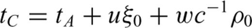
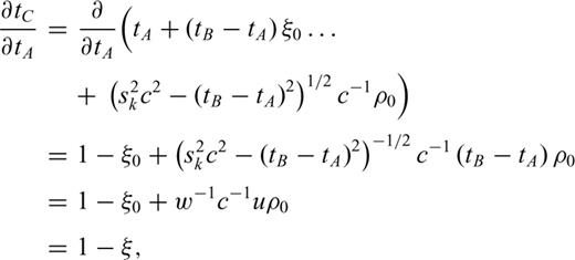
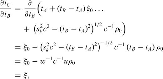
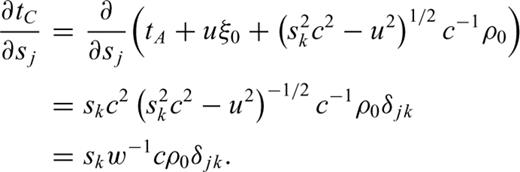
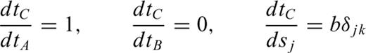
Refer to Fig. 2., ξ is a normalized distance along the line segment from node A to node B (line AB). ξ₀ is the normalized projection of node C onto line AB, and ρ₀ is the length of the normal from node C to the point at ξ₀. The traveltimes at nodes A and B are t_A and t_B, respectively, and are treated as known quantities calculated at previous stages in the FMM solution.

Figure 2

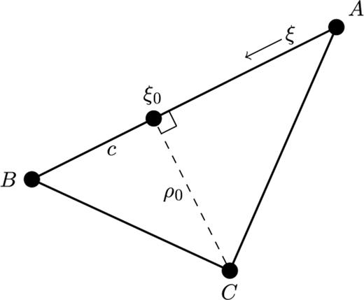
A geometrical scheme for the traveltime updating procedure in 2-D, adapted from Fomel (1997).

Open in new tabDownload slide

We make the common assumption that the wave fronts travelling through the cell are linear such that any rays travelling through the cell are also linear. This assumption leads to first-order modelling accuracy. Although higher-order accuracy can be obtained it complicates the numerical methods and we choose to demonstrate our inversion approach using the simpler case. Under this assumption, the traveltime t_C at the remaining node C is calculated using

2

with

3

where u=t_B−t_A, c is the length of line AB and s is the homogeneous slowness of the triangular cell.

The traveltime in eq. (2) corresponds to a wave transmitted through the cell. The FMM local update considers both the transmitted wave traveltime defined by eq. (2) and traveltimes that can be attributed to the phenomenon of head waves travelling along the sides AC and BC (Podvin & Lecomte 1991)

4

The transmitted wave traveltime is only accepted as a valid option if the solution comes ‘from within’ the triangular cell. This means that ‘the gradient of the solution at a grid point should point into the triangle from which it is updated’ (Kimmel & Sethian 1998). Back-tracing a ray from node C gives an intersection point on face AB at

5

and we need 0 < ξ < 1 to accept the transmitted wave. Furthermore, t_C in eq. (2) is undefined when w² < 0 in eq. (3), the physical meaning of which is discussed in Lelièvre et al. (2010), and in this case the transmitted traveltime is again not accepted as a valid option.

2.3 The local traveltime update on a 3-D tetrahedral grid

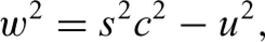
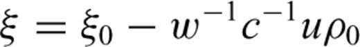
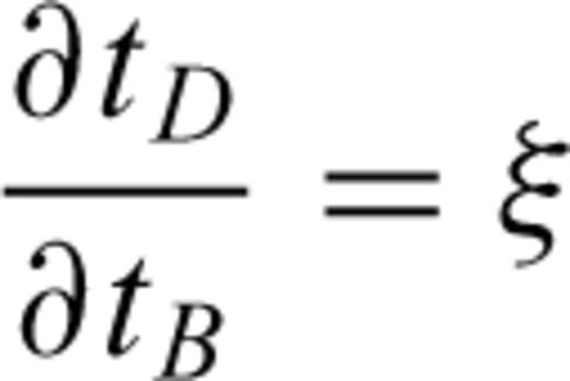
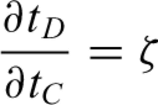
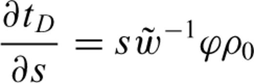
The extension of the local update to 3-D on a grid of tetrahedral cells is provided in detail in Lelièvre et al. (2011). We summarize here. Consider updating the traveltime at a fourth node, D, based on the traveltimes at the nodes belonging to the face opposite node D. Fig. 3 shows the triangular face opposite node D (face ABC). ξ is a normalized distance along line AB, ζ is a normalized distance along line AC and point (ξ₀, ζ₀) is the normalized projection of node D onto face ABC.

Figure 3

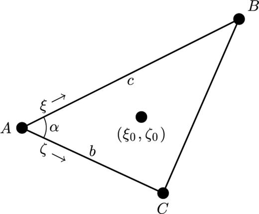
A single face of a tetrahedron opposite a fourth vertex D.

Open in new tabDownload slide

In an analogous manner to the 2-D scenario, wave fronts through the tetrahedral cell are assumed to be planar. The traveltime t_D is calculated using

6

with

7a

7b

where u=t_B−t_A, v=t_C−t_A and ρ₀ is the length of the normal from node D to the point (ξ₀, ζ₀).

Recall that in the 2-D case, the FMM local update generally considers the transmitted wave traveltime defined in eq. (2) and two traveltimes associated with travel along cell edges. In the 3-D case, we must consider six traveltimes in addition to the transmitted wave traveltime. Three of these travel along linear edge elements of the tetrahedron and are calculated as

8

where ∥AD∥ is the distance from node A to node D (with similar definitions for ∥BD∥ and ∥CD∥). The physical interpretation of these traversals is that of diffraction (Podvin & Lecomte 1991). The remaining three waves travel along the triangular face elements of the tetrahedron that connect to node D and are interpreted as head waves. Those head wave traveltimes can be calculated by reducing each triangular face to the 2-D scenario in Section 2.2.

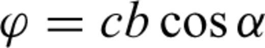
Again, the transmitted wave traveltime is only accepted as a valid option if the solution comes from within the tetrahedral cell and . Back-tracing a ray from node D gives an intersection point on face ABC at a point (ξ, ζ) with

9a

9b

and we need 0 < ξ < 1, 0 < ζ < 1 and ξ+ζ < 1 to accept the transmitted wave.

3 Solution of the Inverse Problem

3.1 A deterministic optimization approach

To invert first-arrival traveltime data, we choose to work in a deterministic framework, where well-behaved functions are minimized through a descent search. This contrasts with a more computationally intensive statistical sampling framework.

The subsurface is discretized into an unstructured grid of many triangular or tetrahedral cells. Let there be M cells and N first-arrival traveltime data. The model vector m holds the slowness values in each cell

10

We follow a typical deterministic procedure of developing an objective function to minimize consisting of a data misfit term and a minimum structure regularization term. The objective function is

11

which, once minimized, should provide a model that fits the observed data to some acceptable degree and contains reasonable spatial characteristics.

The data misfit term,

12

measures the difference between the measured data, d, and the data generated for the candidate slowness model, F[m], where F denotes the traveltime forward modelling operator. The data differences are normalized by estimated uncertainties, σ_i.

Our regularization term is based on that in Li & Oldenburg (1996),

13

The first term controls the closeness of the recovered model, m, to a reference model, m_ref, or in the absence of a reference model it encourages small values in the recovered model. The operator W_s contains the square-root of cell volumes along its diagonal. The second term encourages smoothness in the recovered model. W_m calculates model differences between adjacent grid cells. Each difference is normalized by the distance between the cell centroids and scaled by the square-root of the average volume of the two adjacent cells. The α_s and α_m parameters are held constant throughout an inversion and can be used to encourage different spatial characteristics in the recovered model. In addition to improving the mathematical stability of the inversion, the regularization allows the introduction of prior geological knowledge (Aldridge & Oldenburg 1993).

Selecting a value for the parameter β in eq. (11) represents a trade-off: decreasing values of β yield models that fit the data better but contain more structure, for example, a roughening of the slowness distribution. Pushing β too low can begin to fit noise in the data, leading to spurious structure in the recovered model.

3.2 Constrained optimization

The addition of model-based constraints to the inverse problem is of upmost importance due to the inherent non-uniqueness of the inverse problem. An advantage of posing the inverse problem as above is that it provides the user the ability to incorporate prior geological information into the inversion to constrain the results. This can be achieved through use of the reference model or by inserting weights into the W_s and W_m operators (see Farquharson et al. 2008; Williams 2008). As discussed in Lelièvre (2009), more types of geological information can be incorporated by adding constraints to the optimization problem. For example, upper and lower bounds can be assigned to particular model elements such that the corresponding values in the recovered model must lie within those bounds.

Generally, the preferred route to improve the numerical accuracy of the forward solution would be to use a finer discretization near the sources. However, such fine-scale discretization can easily become infeasbile for large inverse problems such as those that arise in the 3-D real-Earth scenarios of interest to us. Alternately, if one were to include some initialization radius into the FMM solution as mentioned in Section 2.1 then it would be important to apply some form of constraint to the inversion such that the assumption of homogeneity within each near-source region was maintained. This can be achieved by addition of linear constraints into the optimization problem as described by Lelièvre & Oldenburg (2009).

3.3 Minimizing the objective function

To minimize the objective function for some value of β we perform a Gauss–Newton descent search. At each iteration, a search direction p is determined by solving

14

where the gradient, g, and approximate Hessian, H, are the first and approximate second derivatives of the objective function Φ with respect to the model vector m. The model is updated at the kth iteration using

15

where a simple line-search is performed to find a value of the step length parameter η that provides an acceptable reduction in the objective function. When additional constraints are added to the objective function, as mentioned in Section 3.2, the minimization process becomes more involved. However, the solution still relies on a Gauss–Newton descent search and the basic requirement remains being able to provide the gradient and an approximate Hessian.

For the Φ_m term, the required derivatives are trivial. For the Φ_d term they require the quantity

16

(the Gauss–Newton method avoids second derivatives of F[m], which leads to the use of an approximate Hessian). The matrix J contains information about how the traveltime data change as the slowness model changes. This sensitivity information contains a linear component and non-linear component. If rays are traced between each source and receiver pair, and the model is changed by a very small amount, the ray paths will not change appreciably. The data will then effectively vary linearly with the slowness model. However, if the model changes by larger amounts, the ray paths can change, in which case the data show a non-linear variation with the slowness model.

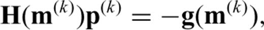
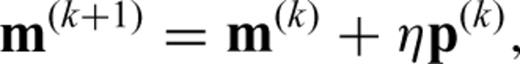
A common approach is to linearize the eikonal equation about the current slowness model such that only the linear sensitivity component is required. This can be calculated in two ways. The typical approach, as discussed in the introduction, is to trace rays through the slowness model. The rays may have already been traced to solve the forward problem, as in Bois et al. (1972), or can be back-traced through the traveltime field resulting from a finite-difference marching method, as in Aldridge & Oldenburg (1993). The ray tracing determines which cells are traversed and the distance of travel through each cell. The matrix J can then be built up from this information but, as we will show, such an approach is not numerically consistent with our forward solution and can therefore cause convergence issues within the inversion resulting from poorly chosen step directions.

Ammon & Vidale (1993) developed an inversion algorithm in which the non-linear sensitivity information is calculated through a brute-force approach. For each cell in the model, they perturb the slowness value, recalculate the forward solution and use a finite-difference approximation for the associated derivative. This approach, although approximate, is attractive in that it maintains numerical consistency between the sensitivity information and the forward modelling method. However, such a brute-force approach carries considerable expensive as it requires a great many forward calculations. This makes it prohibitively expensive for large inversion grids with many cells.

Yet another option is the adjoint-state method, derived by Sei & Symes (1994) and described by Plessix (2006). This approach has a lower cost than a brute-force calculation of the Jacobian, with a cost equivalent to the solution of the forward problem (Taillandier et al. 2009). Leung & Qian (2006) and Taillandier et al. (2009) use this approach when using a Fast Sweeping Method (Zhao 2005) to solve the forward problem.

Finally, we mention automatic differentiation (AD). Sambridge et al. (2007) demonstrated the use of AD to calculate the sensitivities related to ray tracing in a heterogeneous velocity distribution. AD is a method for numerically evaluating the derivative of a function written in a computer coding language. AD looks at the sequence of elementary mathematical assignments in the code and uses the chain rule to combine the trivial derivative expressions for those elementary assignments. The process yields exact derivative information, within numerical accuracy. A huge advantage of AD is that it can provide derivative information at a low cost when symbolically derived expressions are not attainable. On the other hand, an advantage of hard-coding symbolically derived expressions is that the code can often be designed to take advantage of the characteristics of the expressions, for example, by parallelizing the computation wherever possible. Hence, AD may not be the preferred route when code optimization, that is, reduction in memory use and/or run time, is paramount.

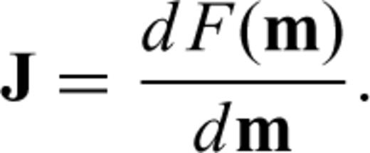
3.4 Calculating sensitivity information directly during the FMM forward solution

Here, we develop an approach for calculating the sensitivity information that maintains numerical consistency with the local updates used in the FMM forward solution. The approach does not require ray tracing and avoids the expense of a brute-force sensitivity calculation. It relies on explicit symbolic differentiation of the forward modelling equations, rather than calculating numerical derivatives, and calculates sensitivity information as the FMM solution marches through the grid.

3.4.1 Two dimensions

For the time being, ignore the actual receiver locations and consider only the traveltimes at each node in the grid. The nodal sensitivity matrix, which we denote J_N (the subscript N for ‘Nodal’), then describes how the nodal traveltimes change as the slowness values within the grid cells change.

To begin, we consider a situation where the FMM solution has progressed part-way through a 2-D grid and we are about to add a new node to the set of upwind nodes. Consider the 2-D local update from Section 2.2 that would have provided a traveltime t_C for this new upwind node. Let s_j denote the slowness in some jth grid cell and let s_k denote the slowness in the cell through which the update was made. The derivative of t_C with respect to some slowness s_j can be calculated by application of the chain rule

17

Assume that the derivatives dt_A/ds_j and dt_B/ds_j have been determined at previous stages in the FMM solution. When a transmitted wave traveltime from eq. (2) is chosen for the update, the remaining partial derivatives are

18a

18b

18c

When a head wave stencil is used for the update, these are

19

or

20

depending on which side of the triangle the chosen head wave travels along. The Kronecker delta, δ_jk, in the expressions above indicates that the only non-zero slowness partial derivative associated with the update is ∂t_C/∂s_k, such that the model partial derivative ∂t_C/∂m is a vector containing only a single non-zero element.

Substituting the expressions in eq. (18) back into eq. (17) we obtain

21

or written in terms of the model vector, m, this is

22

where we denote by e_k a vector with a single non-zero element at the kth position equal to 1. The derivative dt_C/dm in eq. (22) is a single row of the sparse matrix J_N. Computing that row represents a linear combination of previously computed rows of J_N and addition of a constant to one element of the result. The matrix J_N can thereby be built up iteratively during the FMM solution of the forward problem in the same order in which the grid nodes are added to the upwind set.

The characteristics of the FMM allow for such an approach:

• (i)

  once a node is added to the upwind set, the traveltime at that node can no longer be altered;

• (ii)

  traveltime updates at close nodes are calculated using only fixed traveltimes at upwind nodes.

This means that once a row of the matrix J_N is determined it will not change, and any new rows in J_N are computed from previously calculated, and therefore fixed, rows of that same matrix.

To calculate the receiver-based sensitivity matrix, which we denote J_R (the subscript R for ‘Receiver’), consider first the interpolation required to calculate a traveltime at a receiver location within a triangular cell from the three nodal traveltimes in that cell. The interpolation can be calculated as a weighted average

23

where the receiver location is (x, z). One option is to use weights based on distance

24

where r_i is the distance from the receiver to the ith node in the cell. The rows of the matrix J_R can then be generated though linear combination of the rows in J_N using the interpolation weights.

In our computer code, we build J_N row-by-row, keeping track of the order in which the grid nodes are added to the upwind set. We are then able to link each row of the final J_N matrix to specific grid nodes as required when calculating the J_R matrix. Section 4.1 demonstrates the increase in memory required by our new method compared to ray tracing. Use of sparse matrix representation for J_N and J_R means only a moderate increase in memory requirements. To further save on storage and computation time, for each source we stop the FMM solution once all the nodes surrounding the receivers have been moved to the upwind set. Additionally, through careful book-keeping we are able to determine which nodes in the grid affect the traveltime at each receiver as the FMM solution sweeps through the grid, which means that we eliminate the need to calculate and store many extraneous rows of J_N.

3.4.2 Three dimensions

Applying the chain rule in the 3-D situation gives

25

Again, we assume that the derivatives dt_A/ds_j, dt_B/ds_j and dt_C/ds_j have been determined at previous stages in the FMM solution and we require the remaining partial derivatives.

When the local traveltime update on a 3-D tetrahedral grid uses a diffracted wave on a 1-D edge element then the partial derivatives of t_D with respect to t_A, t_B, t_C and s are straightforward. When the update uses a head wave across a 2-D face element then the situation reduces to the 2-D case dealt with above. For the transmitted wave traveltime we have

26

with

27a

27b

The partial derivative with respect to some quantity x is

28

which requires

29

The remaining partial derivatives and ∂s/∂x are all ±1 or 0. Combining the expressions above and making use of the equalities in eq. (9) yields

30a

30b

30c

30d

which are similar to the 2-D case.

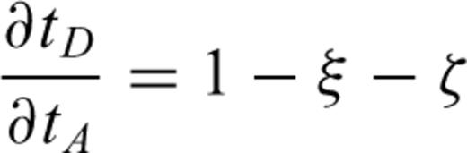
4 Comparison of Sensitivity Calculation Methods

4.1 Numerical comparison

We now compare sensitivities calculated (1) from the FMM local update equations as described above, (2) via ray tracing and (3) though a brute-force calculation as in Ammon & Vidale (1993). The 2-D model for the comparison contains a block within a homogeneous background, as illustrated in Fig. 4. Our coordinate system has +x right and +z down. The modelling region is 200 m by 100 m and the block is 40 m by 40 m, located at the centre of the modelling region (0, 50). A single source is placed on one side of the block at (−90, 50) and a single receiver is placed on the other side at (90, 70).

Figure 4

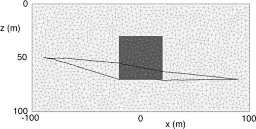
The block model used to compare sensitivity calculations. The anomalous block is dark grey inside a white background. The faces of the triangular cells within the grid are drawn in light grey. Two rays have been traced through the FMM solution traveltime fields and are drawn in black: the upper and lower rays are for the scenarios with anomalously fast and slow block, respectively.

Open in new tabDownload slide

We discretize the model using the freely available meshing program Triangle (Shewchuk 1996; Shewchuk 2002; Shewchuk 2003), constraining the cells to have maximum area of 10.0 m². The grid contains 1649 nodes and 3138 triangular cells. The discretization is somewhat coarse due to the computational requirements of the brute-force calculation. Consequently, the FMM solutions exhibit a significant level of error and the rays traced through the traveltime grid are not ideally straight where expected. However, we are interested here in a numerical comparison, for which this grid will suffice.

We consider two scenarios, one in which the block has a slowness of 1.0 s km⁻¹ within a slower 1.5 s km⁻¹ background, and a second scenario in which the block has a slowness of 1.5 s km⁻¹ with a faster 1.0 s km⁻¹ background. Fig. 4 shows the rays back-traced from receiver to source after the FMM solutions. In the first scenario, the rays preferentially travel through the faster block, refracting as they traverse across the vertical sides of the block. In the second scenario, the faster background presents the optimal travel path and the rays pass along the horizontal sides of the block.

Figs 5–8 compare sensitivities calculated through the three methods mentioned above, with no initialization radius used. The upper limits on the colour scales have been set to the maximum sensitivity values for each calculation. For the brute-force calculation, we perturb each model slowness up and down by some small value δs/2, recalculate the traveltime data via an FMM solution and use central differences to numerically estimate the sensitivities. Here we use a value of δs= 1.0 × 10⁻⁶.

Figure 5

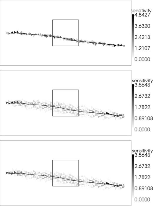
Sensitivities for the block model with an anomalously fast block. Sensitivities are calculated by tracing rays (top panel), through our new approach (middle panel) and though a brute-force method (bottom panel). Sensitivity values are indicated by the colour scales (the units are metres). The outline of the square block is indicated by a thick black line. The rays are drawn in black. Axis labels have been removed to avoid clutter but are as in Fig. 4.

Open in new tabDownload slide

Figure 6

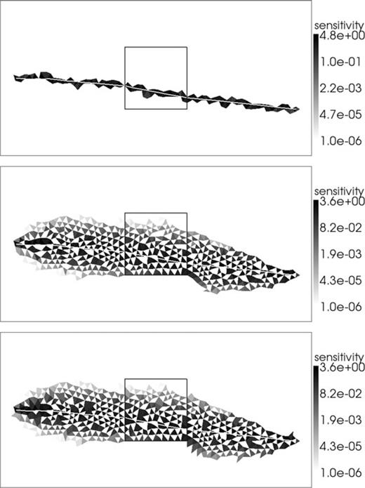
As in Fig. 5 but with logarithmic colour scale and rays drawn in white.

Open in new tabDownload slide

Figure 7

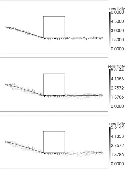
As in Fig. 5 but for the scenario with an anomalously slow block.

Open in new tabDownload slide

Figure 8

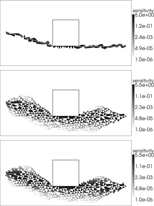
As in Fig. 7 but with logarithmic colour scale and rays drawn in white.

Open in new tabDownload slide

At first glance, the patchy pattern produced by our new method looks problematic. However, further thought indicates that it is fully expected. For any particular node, the FMM algorithm picks the minimum traveltime for several possible wave fronts coming through the cells associated with that node. In the local vicinity of the node, the only cell that effects the traveltime at that node is the cell through which the minimum traveltime is calculated. By picking the minimum traveltime from several possibilities and ignoring the rest, the FMM is effectively turning the sensitivity of some cells off as it marches through the grid.

When it comes to inverting with such patchy sensitivities, one may be concerned that this patchy character may find its way into the recovered models. However, this is easily mitigated by the smoothing involved in minimum structure inversions. Another concern related to inversion is that a small perturbation in the slowness of a particular cell may have a large effect on the sensitivities of those cells downwind from it. A small perturbation may cause a cell with an existing non-zero sensitivity to be switched off and the sensitivity set to zero. This issue of instability results from the fundamentally non-linear nature of the seismic forward problem involved and the same issue therefore exists when using ray tracing to calculate sensitivities: a slight change in the slowness value in one model cell might change the overall ray path considerably. This suggests that implementation of a trust-region might be required in the inversion in order that the sensitivities calculated at a particular iteration remain appropriate over the range of the model perturbation. However, our inversions perform adequately without limiting the perturbation length, suggesting that the level of non-linearity is not severe enough to be problematic.

The ray-traced sensitivity kernels are non-zero in only those cells that lie along the infinitely thin ray paths, which is consistent with the eikonal equation. For our new method there are many more cells with non-zero sensitivity, which leads to increased memory requirements over the ray tracing alternative. Our sensitivities are higher along the ray paths and quickly fall to zero away from them. In Fig. 9, we calculate sensitivities using our new method for the same scenario in Fig. 6 but with finer mesh discretizations. Our sensitivity kernels become more ray-like when the modelling region is more finely discretized, showing that the kernels trend towards a ray-like solution as expected for the eikonal equation, and that the spread in the kernels is associated with numerical modelling error in the FMM solution.

Figure 9

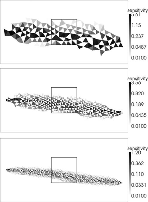
As in Fig. 6 with sensitivities calculated through our new approach and with different grid discretizations. From top to bottom, the maximum cell area supplied to Triangle are 50.0, 10.0 and 2.0 m².

Open in new tabDownload slide

From an inversion perspective, it is best to ensure that the sensitivity information used is numerically consistent with the forward solution. The derivative information in the gradient and Hessian of eq. (14) needs to be numerically consistent with the function being minimized in eq. (11), otherwise the convergence of the minimization can suffer from poor choice of model perturbations. Hence, the sensitivity information incorporated into the Jacobian in eq. (16) needs to be numerically consistent with the local traveltime update equations in Sections 2.2 and 2.3 which are present in the forward solution F(m).

Compare the results for the brute-force calculation against our new method for calculating sensitivities directly from the FMM local update equations. The only numerically significant differences between those two solutions are at or near cells with zero-valued sensitivities in one solution and non-zero sensitivities in the other. This is caused by the non-linear effects mentioned above: when performing the brute-force calculation, small changes in the model sometimes cause the FMM solution to move through different cells. Despite this unavoidable issue, the brute-force calculation confirms the validity of our new method for calculating sensitivities. It is also clear that sensitivities calculated via ray tracing are not numerically consistent with the FMM forward solution and ray-traced sensitivities can only be considered a rough approximation.

We now compare computation times for the sensitivity calculations. To do so, we calculate the sensitivities with increasing levels of discretization. The number of cells in each grid and the computation times for ray tracing and our new method are provided in Table 1. We do not provide calculation times for the brute-force approach as it quickly becomes infeasible as the number of cells in the grid increases. Because the brute-force approach with central differences requires two FMM solutions per grid cell, the computation times are many orders of magnitude higher than for the other methods. The computation times for our new method are an order of magnitude higher than for ray tracing. However, we mention that our research code is written to be simple, robust and extendable, rather than being optimal for speed, and the computation times should be compared with this caveat in mind.

Table 1

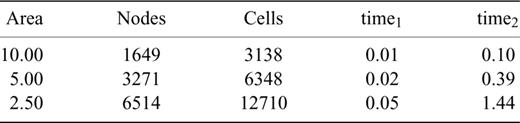
Maximum triangle areas (m²) supplied to Triangle, the resulting number of grid nodes and triangular cells used to discretize themodel in Fig. 4, and CPU computation times (s) for the sensitivity calculations on those grids using a 2.53 GHz dual core machine. The computation times for the ray tracing method and our new method are denoted by time₁ and time₂, respectively. The times here are for the scenario with a faster anomalous block but the times for the other scenario are comparable.

Open in new tabDownload slide

4.2 Comparison of inversion results

Here, we apply our inversion methods to a 2-D example inspired by a scenario from the Voisey's Bay massive sulfide deposit in Labrador, Canada. The model contains several vertically stacked, shallow dipping, lens-like slower bodies (0.23 s km⁻¹) within a faster homogeneous background (0.16 s km⁻¹). The modelling region is 240 × 160 m. A smaller inversion region of 110 × 160 m lies between a line of down-hole sources and a line of down-hole receivers. The sources and receivers are spaced every 10 m down each drillhole. We discretize the model into a triangular grid using the meshing program Triangle, constraining the grid cells to a maximum area of 4.0 m² on both the forward modelling and inversion grids. The forward modelling grid conforms to the outlines of the slower bodies, but the inversion grid does not so that the discretization does not influence the results.

The traveltimes at each receiver, for each source, are calculated using the FMM algorithm. We do not use an initialization radius here. The traveltimes range from 16.0 to 31.9 ms. A small amount of random Gaussian noise is added to the data, with standard deviations (σ_i in eq. 12) equal to 0.32 ms. The data misfit represents a chi-squared variable and therefore we invert by finding a value of the trade-off parameter β that yields an expected value for the misfit close to the number of data. We set the reference model to zero and use α_s = 0.0 and α_m= 1.0.

Fig. 10 shows the true and recovered models. For these inversions we calculated sensitivities through the standard ray tracing approach and through our new method. The ray-traced sensitivity inversion exhibits commonly seen artefacts that have locations and directions connected to the ray traces. These artefacts can not be removed by increasing the weight on the smoothing term in the regularization: the smoothing term is at its relative maximum here (with α_s= 0.0). The smoothing can only be increased with a reduction in data fit, which would cause a smoothing of the larger scale features as well as the ray-like artefacts. In comparison, our alternate approach can reduce such artefacts considerably. This is because it spreads sensitivity information throughout the grid, providing more numerical support between the model and the data, without reducing the resolution of the inversion. We acknowledge that these artefacts are second-order and that major features are common to both solutions. However, such artefacts still have the potential to mislead interpretations.

Figure 10

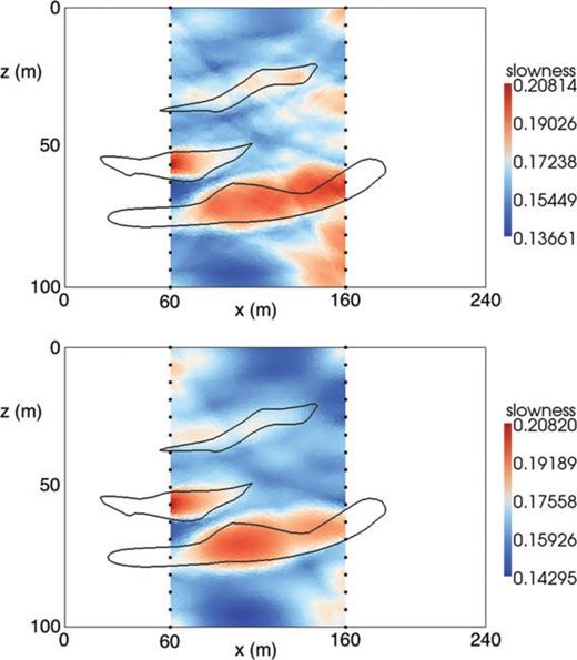
2-D models recovered by inversion using ray tracing (top) and our new approach (bottom) to obtain sensitivities. The outlines of the true bodies are superimposed in black on top of the recovered models. Lines of down-hole sources (left-hand side) and receivers (right-hand side) are displayed as black dots. The colour scales show slowness in s km⁻¹.

Open in new tabDownload slide

Inversion times for a 2.53 GHz dual core machine were 1.2 and 5.8 min for sensitivities calculated using ray tracing and our new method, respectively. The number of non-zeros in the Jacobian for each method, calculated for the true model, was 32 244 and 227 748 respectively. This represents an estimated increase in memory usage for our new method by a factor of 7.1 over the ray tracing method. Although there is a difference in computation time for the Jacobian for the two methods, the majority of the difference is involved in the solution of eq. (14), for which we use the Conjugate Gradient (CG) algorithm. The CG algorithm multiples the Jacobian by vector quantities many times, which represents many more elementary operations for the Jacobian calculated through our new method than for ray tracing due to the increased amount of elements in the sparse Jacobian matrix. The CG algorithm does not require the sensitivity matrix to be provided explicitly, as we do here. Instead, it only needs a method for computing a multiplication of this matrix with a vector, which is the approach effectively provided by the adjoint-state method.

5 3-D Inversion Example

We now present a 3-D synthetic inversion example, again based on the Voisey's Bay massive sulfide deposit but for a different deposit feature. A triangulated surface model for the sulfide ore has been generated from drillcore logging and can be used, along with topography information, to constrain the meshing of our tetrahedral modelling grid. We use surface sources and down-hole receivers, the placement of which is fabricated but representative of a recent field survey, the data from which are not yet available for publication.

Our modelling volume has lateral dimensions of 700 × 400 m. The topography surface lies 170–223 m above the bottom of the volume. We discretize the Earth model into a tetrahedral grid using the TetGen program (Si 2007, 2008a,b, 2010; Si et al. 2010), constraining the grid cells to have a maximum volume of 1000 m³. The resulting grid contains 15 384 nodes and 85 711 tetrahedral cells. Slowness values used for the background and sulfide units are 0.16 and 0.23 s km⁻¹, respectively. As in the 2-D example, we generate an inversion grid that does not conform to the sulfide surfaces so that the discretization does not influence the results. The inversion grid contains 16 512 nodes and 93 033 cells (also using a maximum volume constraint of 1000 m³).

180 seismic sources are draped onto the topography surface on a grid with 40 m spacing. Three drillholes contain 28 receivers, which are spaced down-hole every 20 m. We use the reciprocity theorem to swap the sources and receivers in the forward and inverse modelling. This decreases the computation time considerably because one FMM solution is required for each source. All source–receiver pairs are used for the first-arrival traveltime data. We do not use an initialization radius in the traveltime modelling. The computed traveltimes range from 5.87 to 104 ms. We add a small amount of random Gaussian noise to the data, with standard deviations equal to 0.12 ms plus 2 per cent of the absolute data values. We set the reference model to zero, we use α_s= 0.0 and α_m= 1.0, and we invert to obtain a misfit close to the number of data.

Fig. 11 shows views of the true model and the seismic sources and receivers. Fig. 12 shows slices through the recovered model. The inversion recovers the main ore body and the smaller extension well with only a small amount of additional spurious structure near the down-hole receivers. Much of the apparently patchy character of the slices in Fig. 12 is purely a visual effect resulting from cutting a planar slice through several essentially randomly oriented tetrahedral cells.

Figure 11

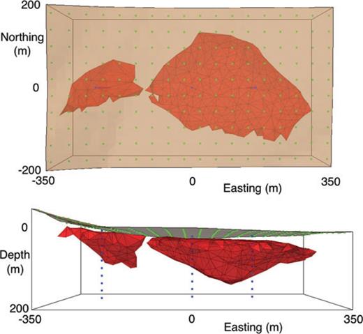
Perspective views of the 3-D model from above (top) and the south (bottom). The main sulfide ore body and smaller extension are red, the topography surface is brown, the boundary of the modelling region is black, seismic sources are green dots and seismic receivers are blue dots. The sulfide and topography surfaces have been made partially transparent so that the sources and receivers can be better seen.

Open in new tabDownload slide

Figure 12

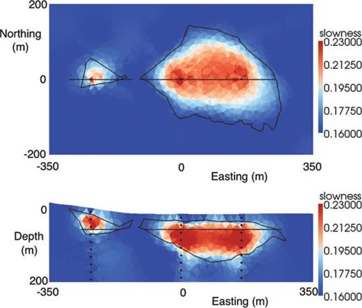
Slices through the 3-D recovered model. Top panel: A horizontal slice at a depth of 60 m. Bottom panel: A west–east vertical slice at northing 0 m. The outlines of the true sulfide surfaces for each slice are shown as black lines. The down-hole receivers are shown as black dots. The colour scales show slowness in s km⁻¹. To aid comparison, we have set the lower and upper colour scale limits to the true slowness values for the background and sulfide units.

Open in new tabDownload slide

6 Discussion

First-arrival ray tracing can be problematic in different situations for several reasons. We have developed a method for inverting first-arrival seismic traveltimes that does not require ray tracing. To achieve this, we solve the forward problem using the Fast Marching Method and we calculate sensitivity information through an explicit symbolic differentiation of the forward modelling equations used. The sensitivities can be calculated directly during the forward solution. This approach is computationally efficient in comparison to a brute force approach, should be comparable in speed to the adjoint-state method, and is not considerably slower than tracing rays.

Calculating the sensitivity information through our new method has advantages over the alternative of tracing rays. It is numerically consistent with the forward modelling equations used and therefore may improve the convergence of the inversion by providing better search directions at each iteration of the minimization. Granted, this leaves us using sensitivity kernels that are not consistent with rays. However, use of the eikonal equation is itself an approximation to the physics of seismic traveltime tomography. In fact, one may consider the spread-out nature of the FMM-derived sensitivities to be a useful property in that it mimics frequency-dependent wave effects.

Our inversion examples have shown that these two choices for calculating the sensitivities can yield models of significantly different character. Specifically, when ray tracing is used it is common to see artefacts in the models that have locations and directions connected with the ray traces. Such artefacts are significantly reduced or absent when our new method is used instead. This is an important result because such artefacts have the potential to mislead interpretations.

Although our method introduces increased memory requirements and computing time, it may be possible to reduce those through thresholding or compression strategies for the Jacobian matrix, although we leave that to future work. As mentioned in Section 3.3, there are alternate approaches for calculating the sensitivity information. These include the adjoint-state method and AD. The choice for one approach over others for a particular application requires experimentation and could be the subject of future work.

Despite the advantage of avoiding ray tracing, grid based modelling holds important limitations that should be considered prior to application; Rawlinson et al. (2007) discuss these limitations in more detail. First, accuracy is a function of grid spacing and is first-order in our methods. As such, computation time may be unacceptably high if high accuracy is required. For real-Earth inversion scenarios, the level of uncertainty in the traveltime data is generally high enough to avoid the need for such high modelling accuracy. Lelièvre et al. (2011) performs error analyses on the forward solution that could be followed when designing modelling grids to address accuracy concerns.

Second, first-arrival traveltimes do not necessarily represent the most energetic arrivals. For some subsurface scenarios, the first-arrival signal may be low compared to noise levels and picking of the first-arrivals may be difficult. Furthermore, first-arrival data contains only a small fraction of the information contained in the full waveform. In applications such as seismic reflection imaging in complex media, the first-arrival solution may not be adequate: see Geoltrain & Brac (1993) and Audebert et al. (1997). Fomel & Sethian (2002), Rawlinson & Sambridge (2004b) and de Kool et al. (2006) develop methods for calculating multiple arrivals using the Fast Marching Method. Future work could attempt to extend our inversion methods when multiple arrivals are considered.

Acknowledgments

We thank Brandon Reid for his help designing the model used for the 2-D inversion example. Financial support for the work presented here was provided by NSERC, the Atlantic Innovation Fund and Vale through the Inco Innovation Centre at Memorial University. This manuscript was improved by helpful and insightful reviews from Sergey Fomel and one anonymous reviewer.

References