Hessian kernels of seismic data functionals based upon adjoint techniques

Summary

1 Introduction

1.1 Full waveform inversion

Full waveform inversion is a tomographic technique that is based on the numerical simulation of seismic wave propagation. The purely numerical solutions of the wave equation for heterogeneous Earth models provide complete and accurate synthetic seismograms that can be exploited for high-resolution imaging in complex media.

While already initiated in the late 1970s and 1980s (e.g. Bamberger et al. 1977, 1982; Tarantola 1984; Gauthier et al. 1986; Tarantola 1988), full waveform inversion has only recently gained popularity, mainly for two reasons: rapid advances in high-performance computing and our need to reveal the structure of the Earth with increasing detail. Applications of full waveform inversion to real data have now been reported in widely varying contexts, ranging from exploration and engineering problems (e.g. Igel et al. 1996; Operto et al. 2004; Gao et al. 2006; Smithyman et al. 2009) to the imaging of regional- and continental-scale structure (e.g. Dessa et al. 2004; Bleibinhaus et al. 2007, 2009; Chen et al. 2007; Tape et al. 2009, 2010; Fichtner et al. 2009, 2010). Despite the success of full waveform inversion, numerous challenges remain. These include the design of more efficient optimization schemes and the rigorous quantification of model resolution and uncertainties.

1.2 Efficiency of optimization schemes and the Newton method

The efficiency of iterative schemes used to minimize the misfit χ between observed seismograms u₀(t) and synthetic seismograms u(t) improved continuously over the past three decades. Simplistic steepest-descent methods employed in the early-development stage of full waveform inversion (e.g. Bamberger et al. 1982; Gauthier et al. 1986) have been replaced by pre-conditioned conjugate-gradient algorithms (e.g. Mora 1987, 1988; Tape et al. 2007; Fichtner et al. 2009) and Newton-like methods (including Gauss–Newton and Levenberg–Marquardt) that use the approximate Hessian (e.g. Pratt et al. 1998; Epanomeritakis et al. 2008; Brossier et al. 2009). The ultimate step to be taken, is the implementation of the full Newton method where the Earth model in iteration k, denoted by m_k, is updated according to

1

where the descent direction h_k is the solution of the Newton equation

2

The symbols H and signify the Hessian and the Fréchet derivative of the misfit functional χ with respect to the Earth model. Newton's method converges quadratically provided that the initial model m₀ is sufficiently close to the global optimum. It therefore has the potential to reduce the number of iterations needed to reach acceptable solutions. While common practice in non-linear optimization (e.g. Hinze et al. 2009), the feasibility of the Newton method in full waveform inversion has so far only been explored in 1-D synthetic studies (Santosa & Symes 1988; Pratt et al. 1998).

1.3 Quantification of resolution

While full waveform inversion is a promising tool, resolution estimates are generally deficient. They are mostly based on synthetic inversions for specific input structures and on the visual inspection of the tomographic images. Synthetic inversions are known to be potentially misleading even in linearized tomographies (Lévêque et al. 1993). Visual inspection is equally inadequate because of the very efficient psychologic trap to mistake the great detail seen in the models as an indicator of comparatively high resolution. In fact, small-scale features may easily appear in full waveform inversion because it hardly requires any explicit regularization—in contrast to classical linearized tomography that is based on the solution of large ill-conditioned linear systems.

Early attempts to analyse—and in fact define—resolution were founded on the equivalence of diffraction tomography and the first iteration of a full waveform inversion (e.g. Devaney 1984; Wu & Toksöz 1987; Mora 1989). However, this equivalence holds only in the impractical case where the misfit χ is equal to the L₂ waveform difference (Fichtner et al. 2008). Furthermore, the analysis of diffraction tomography is feasible only in homogeneous or layered acoustic media.

Despite being crucial for the interpretation of the tomographic images, methods for the quantification of resolution in realistic applications of full waveform inversion do not exist so far. This absence of a quantitative means to assess the capabilities of full waveform inversion is the source of much scepticism as to whether it is really worth the effort.

Part of the problem is the inherently non-linear relation between Earth structure and seismic waveforms that leads to misfit functionals with multiple local minima. At least in the vicinity of the global optimum , characterized by , the Hessian matrix H can be used to infer the resolution of and the trade-offs between model parameters. Approximating χ quadratically around χ yields

3

Furthermore accepting Gaussian statistics, allows us to define a probability density

4

Eq. (4) reveals that is the inverse posterior covariance matrix in the vicinity of (e.g. Tarantola 2005). It follows that contains all the information on resolution and trade-offs, provided that we are sufficiently close to the global optimum.

1.4 Objectives and potentials

The key role played by the Hessian in optimization and resolution analysis motivates the development of methods that allow us to compute the second derivatives of χ with optimal efficiency. When a discretized version of the governing equations can be solved explicitly—as in 2-D frequency-domain modelling (Pratt et al. 1998)—the product of H and an arbitrary model vector can be computed conveniently via an extension of the discrete adjoint method. However, in large-scale 3-D applications where the forward problem is solved iteratively in the time domain, the matrix formalism of the discrete adjoint method becomes impractical.

Our prime objective is therefore to generalize the continuous adjoint method to the computation of the Hessian operator H applied to an arbitrary model perturbation δm. This is intended to serve as a technical preparatory step for future developments, and as a means to gain the intuition and experience needed for the meaningful solution of any inverse problem.

The potential of the method developed in the following sections goes far beyond Newton's method and the quantification of uncertainties. It may as well be used for extremal bounds analysis (Meju & Sakkas 2007; Meju 2009; Fichtner 2010), for the determination of optimal step lengths in gradient-based optimization, as a tool to assess second-order effects on seismic data functionals including finite-frequency traveltimes (see Section 4), to study wave propagation through complex media (e.g. Baig & Dahlen 2004), or to design locally independent model parameters as it is classically done in Partitioned Waveform Inversion (Nolet 1990, 2008).

1.5 Which Hessian?

The term Hessian is frequently used as a synonym for the approximate Hessian, especially in the context of linearized tomography. For the least-squares misfit functional

5

with synthetic data d and observed data d₀, the Hessian matrix H is given by

6

where G is the Jacobian matrix of d, that is, G=∇_md. The full Hessian H reduces to the approximate Hessian

7

either when the relation between d and m is linear (d≈Gm) or in the hypothetical case of zero misfit (d=d₀). It can, however, be shown in both 1-D synthetic inversions (Santosa & Symes 1988) and large-scale 3-D waveform tomographies (Section 5) that can differ substantially from H.

The analysis presented in the following paragraphs goes beyond the linear approximation and the assumption of small misfits. It will allow us to compute the exact second derivatives of any data or misfit functional, thus fully accounting for the generally non-linear relation between Earth models and seismic observables. The distinction between linearization and inherent non-linearity will become most apparent in Section 4 where we consider the second derivatives of finite-frequency traveltimes that are commonly considered to be nearly linearly related to Earth structure.

1.6 Outline

This paper is organized as follows. To set the stage for the computation of second derivatives, and to introduce basic concepts and notations, we start with a condensed review of the standard continuous adjoint method that allows us to express the Fréchet derivative

8

in terms of the regular wavefield u and the adjoint wavefield u^† (Section 2.1). The extension of the adjoint method to the computation of the Hessian operator H applied to a continuous model perturbation δm(x),

9

is then the topic of Section 2.2. Our approach naturally leads to the concept of Hessian kernels, defined as the volumetric densities of Hδm. The transition to the discrete world is made by projecting the Hessian operator H onto the basis functions of the model space to obtain the components of the Hessian matrix H (Section 2.2.2). Up to that point, our development will be deliberately general. This ensures that the formalism can be applied to any PDE-governed physical system in general and to different types of wave equations in particular. Section 3 is concerned with the specific application of the previously derived equations to the 3-D viscoelastic wave equation. We provide explicit formulas for Hessian kernels and we elaborate on their interpretation in terms of second-order scattering from within secondary influence zones. We furthermore highlight relations between Hessian and Fréchet kernels. To illustrate the concept, we provide a series of examples where we computed Hessian kernels for finite-frequency traveltime measurements on both surface and body waves (Section 4). In a realistic full waveform tomography for European upper-mantle structure we demonstrate that the approximate Hessian differs significantly from the full Hessian, even in the vicinity of the optimal model (Section 5). Finally, Appendix A is intended to reveal close relationships between the discrete and continuous adjoint methods for the computation of second derivatives.

2 The Continuous Adjoint Method for First and Second Derivatives

2.1 First derivatives

Variants of the continuous adjoint method applied to seismic wave propagation have been described by several authors (e.g. Tarantola 1988; Tromp et al. 2005; Plessix 2006; Liu & Tromp 2006; Fichtner et al. 2006; Chen 2011). In the interest of generality and compact notation, we derive here a formulation that is independent of the type of wave equation used. For this we consider a wavefield u that depends on the position vector , time t∈T=[t₀, t₁] and on model parameters

10

The model space contains all admissible parameters m(x) =[m⁽¹⁾(x), m⁽²⁾(x), …]. The components m^(α)(x) may, for instance, represent the distributions of density ρ, the P velocity v_P or the S velocity v_S, that is, m(x) =[ρ(x), v_P(x), v_S(x), …]. The semicolon in eq. (10) indicates that u evolves in space and in time, whereas the model parameters are assumed to be fixed for a given realization of u. The wavefield u is linked via the wave equation, symbolically written as

11

to external sources f and the model parameters m. It is commonly not u itself, but a scalar data functional that we are interested in. The data functional can either play the role of a secondary observable or of a misfit functional that quantifies the discrepancy between observed and calculated waveforms. Without loss of generality we can write in the form of an integral over time and space, that is,

12

where we introduced 〈 . 〉 as a short notation for the time-space integral . The derivative of with respect to m in a direction δm follows from the chain rule

13

where

14

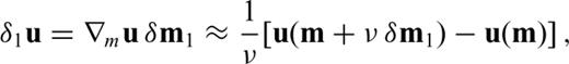
denotes the derivative of u with respect to m in the direction δm. The practical difficulty of eq. (13) lies in the appearance of δu which is often hard to evaluate numerically. For a first-order finite-difference approximation of one needs to determine u(m+εδm) for each possible direction δm. This, however, becomes infeasible in the case of numerically expensive forward problems and large model spaces. Consequently, we may not be able to compute unless we manage to eliminate δu from eq. (13). For this purpose, we differentiate the governing eqs (11) with respect to m. Again invoking the chain rule for differentiation gives

15

The right-hand side of eq. (15) vanishes because the external sources f do not depend on the model parameters m. We now multiply eq. (15) by an arbitrary test function u^† and then apply the integral 〈 . 〉

16

Adding eqs (13) and (16) gives

17

We can rewrite eq. (17) using the adjoint operators ∇_uχ^† and ∇_uL^† which are defined by

18

and

19

for any δu and u^†. We then obtain

20

We may now eliminate δu from eq. (20) if we can determine a field u^† to satisfy

21

Eq. (21) is referred to as the adjoint equation of (11), and u^† and −∇_uχ^† are the adjoint field and the adjoint source, respectively. When the solution u^† of the adjoint equation is found, then the derivative of the objective functional reduces to

22

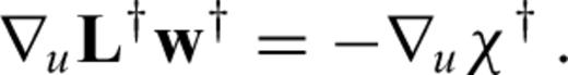
By construction, can now be computed for any differentiation direction δm without the explicit knowledge of δu. This advantage comes at the price of having to find the adjoint operator ∇_uL^† and a solution to the adjoint problem (21). When the operator L is linear in u, it follows that ∇_uL(u)u^†=L^†(u^†), and the adjoint eq. (21) can be simplified to

23

The adjoint field u^† is then determined by the adjoint operator L^† of L and the right-hand side −∇_uχ^† that is derived from the data functional.

2.1.1 Fréchet kernels

Much of our physical intuition is based on the interpretation of sensitivity or Fréchet kernels which are defined as the volumetric densities of the Fréchet derivative

24

In eq. (24), we introduced the dependence of the Fréchet kernel K_m on u and u^† explicitly in the notation. The usefulness of this seemingly unnecessary complication will become apparent the Section 2.2.1 on Hessian kernels. Using the notion of Fréchet kernels, we can recast eq. (22) as follows

25

For the special case of an isotropic Earth model parameterized in terms of ρ, v_P and v_S, eq. (25) takes the form

26

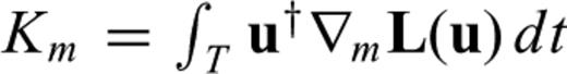
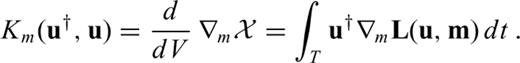
where and are kernels for relative perturbations. The Fréchet kernels reveal how the data functional is affected by infinitesimal changes in the model parameters. It is the study of K_m for different types of seismic waves and different data functionals that allows us to design efficient inversion schemes and to interpret the results in a physically meaningful way.

2.1.2 Translation to the discretized model space

In most applications, the model space is discretized, meaning that the components m^(α) of the space-continuous model m(x) =[m⁽¹⁾(x), m⁽²⁾(x), …] are expressed as a linear combination of N < ∞ basis functions, b_i(x)

27

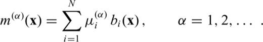
Commonly, the basis functions are spherical harmonics, blocks, wavelets or splines. With the representation (27), the model m and the data functional χ are fully determined by the coefficients or model parameters μ^(α)_i. We are therefore interested in the partial derivatives . Using the definition of the classical derivative, we find

28

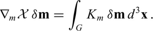
It follows from eq. (28) that the gradient in the classical sense, , is given by the projection of the sensitivity kernel onto the basis function b_i.

2.2 Second derivatives

Equipped with the machinery of the adjoint method for first derivatives, we can now compute the Hessian operator H applied to a model vector δm₁, that is, Hδm₁. For this we first differentiate χ with respect to m in the direction δm₁,

29

with the derivative of the forward field

30

Repeating this procedure for a second direction δm₂ yields

31

with the first derivative

32

and the second derivative of the forward wavefield

33

The first term on the right-hand side of eq. (31),

34

is the approximate Hessian of the data functional χ applied to δm₁ and δm₂. The approximate Hessian merely involves first derivatives that we can already compute efficiently for any differentiation direction with the help of the standard adjoint method that we described in Section 2.1. The Gauss–Newton and Levenberg–Marquardt methods of non-linear optimization use as a computationally less expensive substitute of the full Hessian H.

The difficulty in eq. (31) is the appearance of the second derivative δ₁₂u that we cannot compute efficiently for arbitrary differentiation directions δm₁ and δm₂. To eliminate δ₁₂u from (31) we again differentiate the forward problem, L(u, m) =f, with respect to m in the first direction δm₁

35

Differentiating (35) once more with respect to m but in the direction δm₂ yields

36

In the next step, we multiply eq. (36) with an arbitrary test function w^† and integrate over time and space

37

Adding (37) to (31) and rearranging terms gives

38

We can now eliminate the second derivative of the forward field, δ₁₂u, from eq. (38) by imposing that the test field w^† be the solution of the adjoint equation

39

The adjoint eq. (39) is identical to the adjoint equation for first derivatives (21), which implies w^†=u^†. This means that the adjoint field u^† can in practice be recycled for the computation of the Hessian. When u^† satisfies the adjoint eq. (39), then H(δm₁, δm₂) can indeed be expressed in terms of first derivatives with respect to m

40

The last term on the right-hand side of eq. (40), involving ∇_u∇_uL, is zero for linear operators, including the wave equation operator. Whether the second term, involving ∇_m∇_mL, is zero or not depends on the specific parameterization of the model space. The wave equation operator, for instance, is linear in density and the elastic parameters which leads to a zero second derivative, that is, ∇_m∇_mL=0. However, when the model is parameterized in terms of density and seismic wave speeds, quadratic terms appear and ∇_m∇_mL is generally non-zero.

To apply conjugate gradient type methods to the solution of the Newton eq. (2) we require the Hessian applied to a model perturbation, that is Hδm₁ and not H(δm₁, δm₂). Unfortunately, δm₂ appears implicity via δ₂u in eq. (40). The next step is therefore the isolation of δm₂. For clarity, we restrict the following development to operators L(u) that are linear in u, and we omit the dependence of L on m in the notation. This gives

41

42

43

After slight rearrangements we can now write eq. (40) in the following form

44

Our focus is now on the first two terms on the right-hand side of eq. (44) where the direction δm₂ appears implicitly via δ₂u=∇_mu δm₂. Invoking the adjoint ∇_mL^† of ∇_mL we can write

45

In eq. (45) we have recognized that ∇_u∇_uχ(δ₁u, δ₂u) can be interpreted as a linear operator, ∇_u∇_uχ(δ₁u), acting on δ₂u, that is, ∇_u∇_uχ(δ₁u, δ₂u) =∇_u∇_uχ(δ₁u) δ₂u. To further simplify eq. (45), we differentiate the adjoint eq. (39) with respect to m in the direction δm₁, keeping in mind that L^† is linear in u^†

46

Eq. (46) reveals that the derivative of the adjoint field δ₁u^†=∇_mu^†δm₁ is the solution of an adjoint equation with two source terms on the right-hand side. The first source term, −∇_u∇_uχ^†(δ₁u), is the derivative of the regular adjoint source −∇_uχ^† that we already encountered in eqs (21) and (23). It accounts for the change of the adjoint source that results from the perturbation of the forward wavefield u. The second source term, −∇_mL^†(u^†) δm₁, is located at the perturbation δm₁ itself, and it is responsible for the excitation of a scattered adjoint wavefield (see Figs 2 and 5 for illustrations). We will come back to the physical interpretation of δ₁u^† and its two sources in Section 3.3.2.

Figure 2

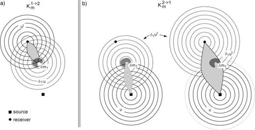
Schematic illustration of the Hessian kernels K^1→2_m and K^2→1_m that are related to first- and second-order scattering. (a) Construction of the Hessian kernel K^1→2_m through the interaction of the the adjoint field u^† and the first-order scattered forward field δ₁u that is generated when the forward field u impinges on the model perturbation δm₁. The Hessian kernel K^1→2_m, shown as the shaded area, localizes the volume where a perturbation δm₂ causes δ₁u to generate a second-order scattered field that affects the measurement at the receiver (•). (b) The Hessian kernel K^2→1_m is the superposition of two influence zones that correspond to the two sources of the differentiated adjoint field δ₁u^†. The first source, −∇_mL^†(u^†) δm₁, excites a scattered field which then generates a secondary influence zone (left panel). A first-order scattered field that originates from within this secondary influence zone can then be scattered again from δm₁ and finally affect the measurement at the receiver. The second source of δ₁u^† is −∇_u∇_uχ^†(δ₁u). The corresponding influence zone extends from source to receiver and accounts for the first-order scattering contribution represented by the approximate Hessian (right panel).

Open in new tabDownload slide

Figure 5

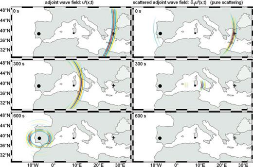
N–S component of the adjoint wavefield u^† (left column) and the pure scattering contribution to δ₁u^† (disregarding the contribution to δ₁u^† from the change of the adjoint source) plotted at the surface. The adjoint wavefield emanates from the receiver (•) and propagates in reverse time towards the source (+). The adjoint source corresponds to the measurement of a cross-correlation time-shift of the N–S component Love wave at a dominant period of 25 s. The location of the v_S perturbation is indicated by ▪. Most of the Love wave energy is scattered forward, that is, in the propagation direction of the adjoint field. The contribution to δ₁u^† that comes from the perturbation of the adjoint source (see eq. 34 and Section 3.3.2) is not shown to enhance the visibility of the pure scattered wave.

Open in new tabDownload slide

With the help of eq. (46) we can simplify eq. (45)

47

To replace L (δ₂u) in eq. (47) we note that the differentiation of the forward problem, L(u, m) =f, with respect to m in the direction δm₂ gives

48

Inserting (48) into (47) leaves us with the following expression

49

where the second differentiation direction, δm₂, appears explicitly. The substitution of (49) into eq. (44) now allows us to assemble the Hessian operator applied to δm₁, that is, Hδm₁

50

The symbol ○ represents a place holder for a second differentiation direction δm₂.

2.2.1 Hessian kernels

Eq. (50) suggests the representation of H(δm₁, δm₂) in terms of volumetric integral kernels that are reminiscent of the Fréchet kernels introduced in eqs (24) and (25)

51

with the Hessian kernels defined by

52

53

54

55

In this sense, we may identify the Hessian operator H applied to the model perturbation δm₁ with the Hessian kernels, that is

56

Considering again the special case of an isotropic medium parameterized in terms of ρ, v_P and v_S, eq. (51) can be written as

57

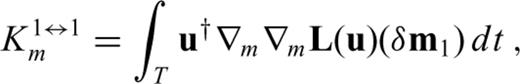
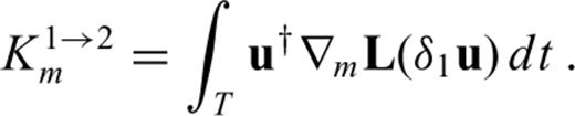
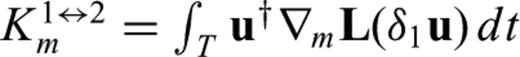
with the kernels for relative perturbations and . Unlike Fréchet kernels, Hessian kernels depend on the model perturbation, δm₁, either explicitly as in K^1↔1_m or implicity via δ₁u and δ₁u^†. The comparison of eqs (53) and (55) with eq. (24) reveals that the Hessian kernels K^2→1_m and K^1→2_m are closely related to the Fréchet kernel K_m. In fact, we find

58

and

59

The explicit formulas derived in Section 3.2 for the Fréchet kernels with respect to specific Earth model parameters can thus be reused for the computation of the Hessian kernels K^2→1_m and K^1→2_m. Eqs (58) and (59) are also important for the physical interpretation of the Hessian kernels.

2.2.2 Translation to the discretized model space

In a discretized model space the components m^(α)(x) of the space-continuous model m(x) are expressed in terms of a linear combination of a finite number of basis functions, b_i(x), as introduced in eq. (27). With the help of the Hessian operator H we can then compute the components of the Hessian matrix H. The component (H)^(αβ)_ij of H is the second derivative of the data functional with respect to the discrete model parameters μ^(α)_i and μ^(β)_j, that is

60

Making use of eq. (28) we find

61

The component (H)^(αβ)_ij of the Hessian matrix is therefore equal to the Hessian operator applied to the basis functions b_i and b_j. It follows that the Hessian kernel K¹_m for the model perturbation δm₁=b_i can be interpreted as a continuous representation of the ith row of the Hessian matrix H.

The derivation of the adjoint equations in the continuous space followed by the discretization through projection is characteristic for time-domain full waveform inversion. This approach differs from frequency-domain full waveform inversion where the discrete adjoint method is applied to a semi-discrete version of the governing equations. That the continuous and discrete adjoint methods for both first and second derivatives are closely related will be shown in Appendix A.

3 Application to the Seismic Wave Equation

Our developments have so far been general in the sense that the equations do not depend on the particular type of wave equation used to model seismic wave propagation. In the following paragraphs, we will be more specific and apply the adjoint formalism to the 3-D viscoelastic wave equation.

3.1 Governing equations and their adjoints

The propagation of seismic waves in the Earth can be modelled with the seismic wave equation

62

that relates the displacement field u in the Earth to its mass density ρ, the stress tensor σ and an external force density f[see Dahlen & Tromp (1998), Kennett (2001) or Aki & Richards (2002) for detailed derivations of eq. 62]. The wave operator L is linear in u. The free surface boundary condition imposes that the normal components of the stress tensor σ vanish at the surface ∂G of the Earth, that is, σn|_x∈∂G=0, where n is the unit normal on ∂G. Both the displacement field u and the velocity field are required to satisfy the initial condition of being equal to zero prior to t= 0: . To obtain a complete set of equations, the stress tensor σ must be related to the displacement field u. For this we assume that σ depends linearly on the history of the strain tensor

63

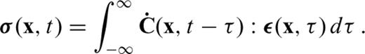
The symbol : in eq. (63) denotes the contraction over the two innermost indices, that is, . Eq. (63) defines a linear viscoelastic rheology. The fourth-order tensor C is the elastic tensor. Since the current stress cannot depend on future strain, we require the elastic tensor to be causal: C(t)|_t<0=0. The symmetry of ε, the conservation of angular momentum and the relation of C to the internal energy (Aki & Richards 2002) require that the components of C satisfy a set of symmetry relations, C_ijkl=C_klij=C_jikl, that reduce the number of independent components to 21. The number of non-zero independent elastic tensor components, or elastic parameters, determines the anisotropic properties of the elastic medium (e.g. Babuška & Cara 1991).

The adjoint wave operator L^†, that governs the propagation of the adjoint wavefield, is given by (Tarantola 1988; Tromp et al. 2005; Plessix 2006; Fichtner et al. 2006)

64

with the adjoint stress tensor defined by

65

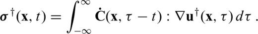
Just as the regular stress tensor σ, the adjoint stress tensor σ^† is required to satisfy the free surface boundary condition σ^†n|_x∈∂G=0. Furthermore, the propagation of the adjoint wavefield is constrained by the terminal conditions , where t_e is the time when the observation ends. In non-dissipative media the elastic wave operator L is self-adjoint, meaning that L=L^†. The obvious numerical difficulty in solving the adjoint equation is the occurrence of the terminal conditions that require that the adjoint field be zero at time t=t_e. In practice, this condition can only be met by solving the adjoint equation backwards in time, that is by reversing the time axis from 0 →t_e to t_e→ 0. The terminal conditions then act as zero initial conditions, at least in the numerical simulation. Eq. (65) reveals that the adjoint stress tensor σ^† at time t depends on future strain from t to t_e. This results in a growth of elastic energy when the wavefield propagates in the regular time direction from 0 to t_e. In reversed time, however, the elastic energy decays, so that numerical instabilities do not occur (Tarantola 1988). For efficient strategies to solve the adjoint equation and the time integral that appears in the Fréchet kernels, the reader is referred to Griewank & Walther (2000), Liu & Tromp (2006) or Fichtner et al. (2009).

3.2 First derivatives and Fréchet kernels

The most general expression for the derivative of a data functional in the direction δm is given by eq. (22) that we repeat here for convenience

66

Substituting the governing eqs (62) and (63) for the general operator L yields the explicit formula

67

with the model perturbation δm= (δρ, δC). To avoid clutter, we omitted spatial dependencies in the notation. Integrating by parts provides a more symmetric and more useful version of eq. (67)

68

where the adjoint strain tensor ε^† is defined by . The Fréchet kernels associated with (68) are

69

and

70

The symbol ⊗ signifies the tensor or dyadic product. Both kernels are non-zero only within the primary influence zone where the regular and adjoint wavefields interact at some time between t= 0 and t=t_e. The primary influence zone, illustrated in Fig. 1, is the region where a model perturbation δm causes the regular wavefield u to generate a first-order or single-scattered wave that affects the measurement at the receiver. A perturbation located outside the primary influence zone has no first-order effect on the measurement.

Figure 1

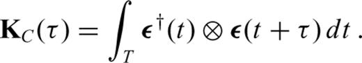
Schematic illustration of the primary influence zone where the regular wavefield u interacts with the adjoint wavefield u^†. Numbers are used to mark the regular and adjoint wave fronts at successive points in time. As time goes on, the regular wavefield propagates away from the source while the adjoint wavefield collapses into the receiver. In numerical simulations the adjoint equations are solved backwards in time to satisfy the terminal conditions. On the reverse time axis, the adjoint field propagates away from the receiver, starting at the final observation time. The primary influence zone marks the region where a model perturbation δm generates a first-order scattered wavefield that affects the measurement at the receiver. Perturbations located outside the primary influence zone have no first-order effect on the measurement. The spatial extension of the primary influence zone is proportional to the length of the analysis time window considered in the seismograms.

Open in new tabDownload slide

For most seismic phases, the primary influence zone is a roughly cigar-shaped region connecting the source and the receiver. Its precise geometry depends on many factors including the frequency content, the length of the considered time window, the type of measurement and the reference Earth model, m. Specific examples for common seismic phases and measurements can be found, for instance, in Friederich (1999), Zhou et al. (2004), Yoshizawa & Kennett (2005), Zhao et al. (2005), Liu & Tromp (2006, 2008), Nissen-Meyer et al. (2007), Sieminski et al. (2007a,b) or Zhou (2009).

3.2.1 Perfectly elastic and isotropic medium

Eq. (68) is of general validity. The most relevant special case, that we will use for illustration, is the perfectly elastic and isotropic medium. Perfect elasticity means that the time-dependence of the elastic tensor C and its perturbation δC has the form of a unit-step or Heaviside function H(t)

71

Upon inserting (71) into eq. (68) we obtain a simplified expression for

72

In an isotropic medium the components of C are given by (Aki & Richards 2002)

73

The symbols λ and μ denote the Lamé parameters. It follows that the complete derivative of is composed of three terms

74

with

75a

75b

75c

The symbol tr ε signifies the trace of the strain tensor ε. The associated Fréchet kernels are

76a

76b

76c

The superscript ⁰ symbolizes that the Fréchet kernels correspond to the fundamental parameterization m= (ρ, λ, μ). Based on eqs (75) and (76) we can deduce the Fréchet kernels for a perfectly elastic and isotropic medium that is parameterized in terms of density ρ, the S wave speed and the P wave speed

77a

77b

77c

3.3 Second derivatives and Hessian kernels

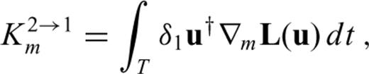
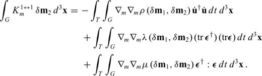
As we have seen already in Section 2.2.1, the second derivative H(δm₁, δm₂) can be conveniently expressed in terms of three Hessian kernels, K^2→1_m, K^1→2_m and K^1↔1_m. It follows from eqs (58) and (59) that we can reuse the formulas for Fréchet kernels from Section 3.2 to compute the Hessian kernels K^2→1_m and K^1→2_m for specific Earth model parameters. The only difference is the involvement of the scattered adjoint field δ₁u^† and the scattered forward field δ₁u in the kernel calculations.

Some additional work is required for the kernel K^1↔1_m: As a preparatory step towards explicit expressions for special rheologies, we substitute the governing eqs (62) and (63) into the definition of K^1↔1_m (eq. 54)

78

In eq. (78) we did not specify a particular parameterization. This is accounted for by the notations ∇_m∇_mρ and that allow ρ and C to depend on model parameters m other than density and the elastic coefficients themselves. Integrating eq. (78) by parts and writing the resulting expression in terms of the regular and adjoint strain fields, ε and ε^†, gives

79

Eq. (79) is, just as eq. (68) for the first derivative , of general validity. Special cases can be derived by further specifications of the rheology, that is, the elastic tensor components and their time dependence. Again, we consider the perfectly elastic and isotropic case as an example.

3.3.1 Perfectly elastic and isotropic medium

First, we substitute the perfectly elastic and isotropic rheology, as described by eqs (71) and (73), into the general expression (79)

80

When the isotropic medium is parameterized in terms of ρ, λ and μ or, alternatively, ρ, κ and μ, we find

81

meaning that the Hessian kernel K^1↔1_m is identically zero. This result depends critically on the choice of the free parameters. Changing, for instance, the set of free parameters to ρ, v_iP and v_iS, results in

82

with the model vector

83

and the auxiliary variable γ_ijkl defined by

84

This allows us to write eq. (80) in a very convenient form

85

where we defined the symmetric 3 × 3 matrix J through

86

From eq. (85) we immediately infer that the Hessian kernel K^1↔1_m is explicitly given by

87

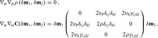
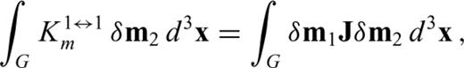
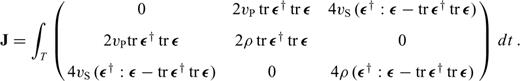
It is interesting to note that the P and S wave speed Fréchet kernels, and , from paragraph (3.2) reappear in the matrix J. In fact, we may write J in the following form

88

The Fréchet kernels for the isotropic medium can thus be recycled for the computation of the Hessian kernel K^1↔1_m.

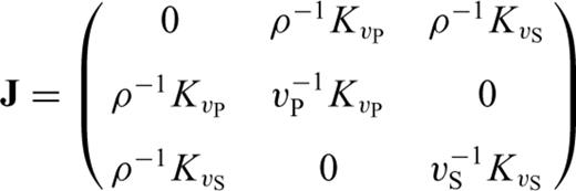
3.3.2 Physical interpretation of the Hessian kernels

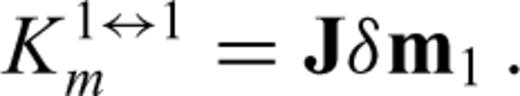
As mentioned in Section 3.2, Fréchet kernels can be interpreted in terms of first-order scattering from within a primary influence zone (see Fig. 1). Hessian kernels, in contrast, also represent second-order scattering from within secondary influence zones. More specifically, the Hessian kernel results from the interaction of the adjoint field u^† with the first-order scattered field

89

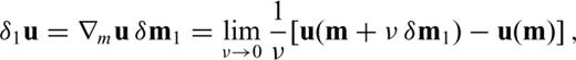
that is excited when the forward field u impinges upon the model perturbation δm₁. The construction of K^1→2_m is very similar to the construction of the Fréchet kernel which involves u^† and u instead of u^† and δ₁u. This similarity suggests that the Hessian kernel K^1→2_m localizes a secondary influence zone where a model perturbation δm₂ can cause the first-order scattered field δ₁u to generate a second-order scattered field that affects the observation at the receiver. Fig. 2(a) illustrates this process.

The interpretation of the Hessian kernel is slightly more involved because the field δ₁u^† has two sources, as we have seen already in eq. (46).

One of the two sources, −∇_mL^†(u^†) δm₁, excites a scattered adjoint field that is similar to the scattered forward field δ₁u but propagates in the opposite direction. The interaction of the scattered adjoint field with the forward field u generates another secondary influence zone that connects the perturbation δm₁ to the source. Another perturbation δm₂ located within this secondary influence zone causes the forward field u to excite a first-order scattered field δ₂u which then interacts with the perturbation δm₁ such that the resulting second-order scattered field affects the measurement made at the receiver. This is shown schematically in the left part of Fig. 2(b).

The second source of δ₁u^† is −∇_u∇_uχ^†(δ₁u), which is the derivative of the regular adjoint source. It accounts for the changes of the adjoint source that are due to the perturbation of the forward wavefield u, and it generates an influence zone that extends from the source to the receiver (Fig. 2b, right-hand side). A comparison with eq. (34) reveals that −∇_u∇_uχ^†(δ₁u) can be interpreted as the source of the approximate Hessian which accounts for the first-order scattering contribution to the full Hessian H.

The complete Hessian kernel K^2→1_m is thus a superposition of (1) a secondary influence zone that corresponds to second-order scattering, and (2) a primary influence zone that corresponds to the first-order scattering represented by the approximate Hessian.

In the interest of a simplified vocabulary, we will henceforth refer to the wavefield

90

as the scattered adjoint field, though keeping in mind that it is caused by more than scattering sensu stricto.

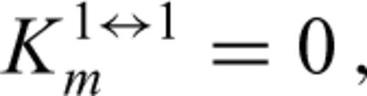
The Hessian kernel does not appear to have a straightforward intuitive interpretation. It accounts for the non-linearity introduced by the parameterization. Whether is zero or not, depends strongly on the choice of free parameters, as we have seen already in Section 3.3.1.

4 Hessian Kernel Gallery

To bring the previous developments to life, we continue with specific examples of Hessian kernels for a small selection of data functionals and model perturbations. Given the infinite number of seismic data functionals and Earth model parameterizations, our Hessian kernel gallery can naturally not be exhaustive. We nevertheless hope that it provides both physical intuition and a useful illustration of the methodology outlined in Sections 2 and 3.

4.1 Surface wave interaction with point-localized and extended scatterers

We begin with a detailed example where we consider a N–S component Love wave excited by a shallow event at 10 km depth and observed at an epicentral distance of 25.2° (Fig. 3, left-hand side). To quantify the discrepancy between the observed waveform u⁰(t) and the synthetic waveform u(t), we measure the cross-correlation time shift , defined as the global maximum of the correlation function

91

We have when the synthetic waveform arrives later than the observed waveform, and when the synthetic waveform arrives earlier than the observed waveform. Under the assumption that u⁰(t) and u(t) are merely shifted in time without being otherwise distorted with respect to each other, the adjoint source corresponding to the data functional is given by (Luo & Schuster 1991)

92

where e_NS and x^r denote the unit vector in N–S direction and the receiver location, respectively. The normalization by the squared L₂ norm ensures that the resulting Fréchet kernels do not depend on amplitude. Treating observed and synthetic waveforms as time-shifted versions of each other is a simplified but widely used approach because it leads to kernels that are quasi-independent of the actual data. We can thus compute kernels without explicitly measuring a time shift.

Figure 3

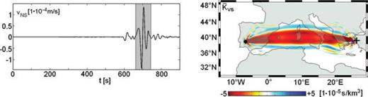
Left-hand side: N–S component synthetic seismogram computed using a spectral-element method (Fichtner & Igel 2008). The time window around the Love wave used to compute Fréchet and Hessian kernels is shaded in grey. The dominant period is 25 s. Right-hand side: Fréchet kernel for a cross-correlation time-shift measurement on the N–S component Love wave shown to the left-hand side. The source and receiver positions are marked by + and •, respectively.

Open in new tabDownload slide

The computation of the Fréchet kernels follows a well-known recipe. First, we solve the forward problem (eqs 62 and 63) to obtain the forward field u that is stored at sufficiently many time steps. Snapshots of u, computed with the help of a spectral-element discretization of the seismic wave equation (Fichtner & Igel 2008), are shown in the left panel of Fig. 4. We then select a time window around the waveform of interest (Fig. 3, left-hand side) and compute the adjoint source given in eq. (92). The adjoint source f^† is the right-hand side of the adjoint eq. (21), the solution of which is the adjoint field u^†, shown in the left panel of Fig. 5. While the adjoint field propagates in reverse time, the previously stored forward field is loaded and used to compute the Fréchet kernels according to eqs (76) and (77).

Figure 4

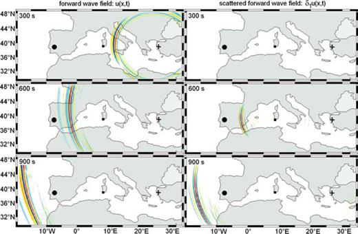
N–S component of the forward wavefield u (left column) and the scattered forward wavefield δ₁u plotted at the surface. The source is marked by + and the receiver by • (epicentral distance =25.2°). The location of the v_S perturbation is indicated by ▪. The images are dominated by surface waves. Small-amplitude body waves are hardly visible. The v_S perturbation acts as a point scatterer (Rayleigh scattering), and most of the Love wave energy is scattered in the forward direction.

Open in new tabDownload slide

The S velocity kernel corresponding to the cross-correlation time shift measurement on the N–S component Love wave is shown in the right panel of Fig. 3. The kernel is dominated by negative sensitivities within the first Fresnel zone, where a positive v_S perturbation leads to earlier-arriving waveforms and to a decrease in the cross-correlation time shift . The width of the first Fresnel zone is proportional to , where T_d and ℓ denote the dominant period and the length of the ray path between source and receiver, respectively.

The Hessian kernel K^1↔1_m can be computed directly from the Fréchet kernels (eq. 88). Additional simulations are needed for K^1→_m² and K^2→_m¹ because these involve the scattered forward field δ₁u and the scattered adjoint field δ₁u^† (eqs 58 and 59). Both scattered fields can be computed most conveniently with the help of the finite-difference approximations

93

and

94

where ν > 0 is a sufficiently small scalar. In our example, we choose δm₁ to be a 10 per cent v_S perturbation, δv_S1, located within a 50 × 50 × 50 km³ box-shaped basis function right beneath the surface at nearly equal distance from the source and the receiver (Figs 4 and 5). The v_S perturbation almost acts as a point scatterer because its dimension is small compared to the dominant wavelength of around 130 km. We are therefore close to the Rayleigh scattering regime. The scattered forward field δ₁u is excited when the regular wave front reaches δv_S1 which acts as a fictitious source. It then propagates towards the receiver (Fig. 4, right-hand side). In contrast, the pure scattering contribution to δ₁u^† collapses into the v_S perturbation δv_S1 (Fig. 5).

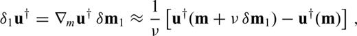
The resulting Hessian kernels and are shown separately in the top row of Fig. 6. The kernel is a superposition of two contributions, labelled F and S. These correspond to the primary influence zone represented by the approximate Hessian (F) and to the secondary influence zone where second-order scattering affects the measurement (See Fig. 2 for a schematic representation). The kernel only extends from the receiver to δv_S1. Second-order scattering from δv_S1 to an S velocity perturbation within has an effect on the measurement. The kernel is restricted to the volume occupied by δv_S1. The complete Hessian kernel is shown in the bottom row of Fig. 6.

Figure 6

Hessian kernels plotted at the surface of the Earth. The position δv_S1 is indicated by ○. Top row: The individual Hessian kernels and (from left-hand side to right-hand side). The kernel has two contributions, labelled F and S. Contribution F represents the primary influence zone that corresponds to the approximate Hessian. Contribution S, encircled by a dotted curve, is a secondary influence zone where second-order scattering affects the measurement. (In Section 5.1, we show how the approximate Hessian can be computed separately.) Bottom row: Composite Hessian kernel . The the contribution from second-order scattering is again encircled by a dotted curve and marked with S.

Open in new tabDownload slide

An interesting observation is that the sign of within the secondary influence zones is opposite (positive) to the sign within the primary influence zone (negative) that corresponds to the approximate Hessian. The widths of the secondary influence zones is proportional to and , where the ℓ_s→1 and ℓ_1→r signify the length of the ray paths from the source to δv_S1 and from δv_S1 to the receiver, respectively. This explains why the secondary influence zones are slim compared to the primary influence zone (labelled F in Fig. 6) where the width is proportional to .

The Hesian kernel K¹_m shown in Fig. 6 can be interpreted as the continuous representation of the row of the Hessian matrix H that corresponds to the basis function coincident with δv_S1. The fully discrete row is obtained by projecting K¹_m onto the basis functions, according to eq. (61).

The amplitude of the Hessian kernel for #x03B4;v_S1 located near the centre of the first Fresnel zone is about two orders of magnitude smaller than the amplitude of the Fréchet kernel. This suggests that the single-scattering approximation is well justified in this particular scenario. Locating δv_S1 further away from the first Fresnel zone rapidly decreases the amplitude of the corresponding Hessian kernels, as can be seen in Fig. 7. The small second derivatives result from the long propagation distance of the scattered waves that arrive too late to have a significant effect inside the Love wave time window (Fig. 3, left-hand side).

Figure 7

Hessian kernel corresponding to an S velocity perturbation δv_S1 that is located in the outer rim of the Fréchet kernel shown in Fig. 3. The position δv_S1 is indicated by ○. The amplitude of is one order of magnitude smaller than in Fig. 6 where δv_S1 was located near the centre of the first Fresnel zone of the Fréchet kernel.

Open in new tabDownload slide

The recipe for the computation of Hessian kernels is equally applicable when the model perturbation (or basis function) does not effectively act as a point scatterer, as in the previous example. For a spatially extended model perturbation δv_S1, such as the one shown in Fig. 8, we are in the Mie scattering regime where the characteristic size of the scatterer is much larger than the dominant period. To calculate the Hessian kernel corresponding to δv_S1, we again compute the scattered fields δ₁u and δ₁u^† using the finite-difference approximations from eqs (93) and (94), respectively. The finite-difference step length ν must be sufficiently small to ensure the convergence of the approximation. For the specific perturbation in Fig. 8, we found ν= 1/100 to be appropriate.

Figure 8

Horizontal (top) and vertical (bottom) slice through the extended v_S perturbation used to compute the Hessian kernel shown in Fig. 9. The maximum perturbation of 0.4 km s⁻¹ near the surface is equal to 10 per cent of the background S velocity.

Open in new tabDownload slide

Slices through the resulting Hessian kernel are shown in Fig. 9. As expected for Love waves, the Hessian kernel is largest near the surface and decays rapidly with increasing depth. An interesting observation is the strong asymmetry of the Hessian kernel, as compared to the one computed for an effective point scatterer (Fig. 6). The origin of the asymmetry is difficult to identify on the basis of purely numerical simulations, though we hypothesize that it is related to the non-isotropic radiation pattern of the regular source.

Figure 9

Horizontal (left-hand side) and vertical (right-hand side) slices through the Hessian kernel that corresponds to the v_S perturbation shown in Fig. 8.

Open in new tabDownload slide

4.2 P body waves and the second-order effect of density

The application of the previously described methodology to other types of seismic waves is straightforward and merely requires the choice of different time windows. In the following example, we consider the measurement of a cross-correlation time shift on the vertical component of an 8 s P body wave in the same source–receiver geometry as above. We furthermore extend the analysis to the multiparameter case. The Fréchet kernels for v_P, v_S and ρ are displayed in Fig. 10(a). As expected, the P wave traveltime is mostly affected by perturbations in v_P, whereas variations in v_S and ρ have hardly any first-order effect.

Figure 10

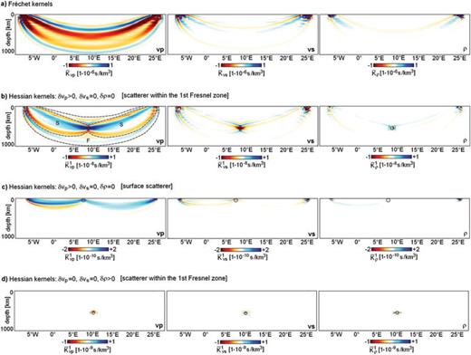
Fréchet and Hessian kernel gallery for the cross-correlation time-shift on the vertical component of an 8 s P wave. The source–receiver geometry is the same as in Fig. 3. (a) Fréchet kernels for v_P, v_S and ρ (from left-hand side to right-hand side). (b) Hessian kernels and (from left-hand side to right-hand side) for a v_P perturbation δv_P1. The position of δv_P1 is indicated by ○. In the kernel the contributions from the second-order scattering and the approximate Hessian are outlined by dash-dotted curves and labelled S and F, respectively. The amplitudes of and are small compared to the amplitude of . (c) The same as in (b) but for a v_P perturbation located directly beneath the surface (○). The kernels are comparatively small but different from zero, indicating that second-order scattering from far outside the Fréchet kernel may affect the measurement because the P wave window is sufficiently long (∼15 s). (d) Hessian kernels and (from left-hand side to right-hand side) for a density perturbation δρ₁. The position of δρ₁ is indicated by ○. The kernels are characterized by rapid variations that are localized around the density perturbation. Compared to the Hessian kernels for a v_P perturbation in (b), the density Hessian kernels have small amplitudes, indicating that ρ has hardly any second-order effect on the finite-frequency traveltime of P waves.

Open in new tabDownload slide

To study second-order effects on the finite-frequency traveltime of the P wave, we again place a 50 × 50 × 50 km³P velocity perturbation, δv_P1, in the centre of the first-order first Fresnel zone of the v_P Fréchet kernel . The dimension of δv_P1 is small compared to the wavelength (∼100 km), meaning that we are close to the Rayleigh scattering regime. The corresponding Hessian kernels, shown in Fig. 10b, contain two symmetric lobes that meet at the location of the scatterer. These lobes correspond to the second-order scattering contribution to the Hessian, and are labelled S in the kernel. The contribution from the approximate Hessian, labelled F, is clearly visible only in . The Hessian kernels and K¹_ρ are small compared to . This indicates that second-order scattering from perturbations of different nature, that is, one perturbation in v_P and another one in ρ or v_S, is rather inefficient.

For a scatterer located outside the first Fresnel zone, we observe a similar decrease of the Hessian kernels as for surface waves (see Fig. 7). In the specific case of a v_P perturbation near the surface, the corresponding Hessian kernels are around two orders of magnitude smaller than the kernels for δv_P1 located in the centre of the Fréchet kernel (Fig. 10c). The fact that scattering from near the surface affects the traveltime measurement at all, can be explained with the finite-frequency content of the P waveform. Doubly-scattered energy from δv_P1 and another v_P perturbation located within the support of can still arrive in the measurement window of the P wave that is around 15 s long.

The kernels shown in Figs 10(a) and (b) reveal that density perturbations have hardly any effect of the finite-frequency traveltime of P waves through first-order scattering or second-order scattering that also involves a P velocity perturbation. To see whether second-order scattering from two density perturbations can influence the P wave traveltime, we repeat the example from Fig. 10(b), but we replace δv_P1 by a density scatterer δρ₁. The resulting Hessian kernels, shown in Fig. 10(d), are practically zero, thus indicating that variations in density do not have any significant second-order effect on P wave traveltimes at all.

This observation is closely related to the characteristics of Rayleigh scattering from density perturbations (e.g. Wu & Aki 1985; Tarantola 1986). For δρ₁≠ 0 and δv_P1=δv_S1= 0 most of the energy is scattered in the direction opposite to the propagation direction of the incident wave (Fig. 11). Therefore, the scattered forward field δ₁u does not interact with the adjoint field u^†, and the partial Hessian kernel K^1→2_m is close to zero. Similarly, the scattered adjoint field δ₁u^† propagates in a direction opposite to the adjoint field u^†, so that the interaction of δ₁u^† with the forward field u is not possible. It follows that K^2→1_m is approximately zero as well. Finally, we have K^1↔1_m= 0 for pure density perturbations (eq. 88), and the complete Hessian kernel K¹_m=K^2→1_m+K^1↔1_m+K^1→2_m nearly vanishes.

Figure 11

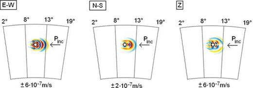
Vertical slices through the E–W (left-hand side), N–S (centre) and Z components of the scattered velocity field . The snapshots are taken 30 s after the P wave reached the density perturbation δρ₁, marked by ○. The direction of the incident P wave is indicated by left-pointing arrows. Clearly visible is the backward scattering associated with δρ₁ > 0 and δv_S1=δv_P1 = 0. Hardly any energy is scattered in the propagation direction of the regular wavefield u.

Open in new tabDownload slide

5 Full Hessian Versus Approximate Hessian

The approximate Hessian is commonly used as a computationally less expensive substitute of the full Hessian H, because its computation merely requires first derivatives. To explore the potential differences between and H, we consider—as an example—a realistic 3-D full waveform tomography. As a preparatory step, however, we expand on the computation of approximate Hessian kernels, using the methodology developed in Sections 2 and 3.

5.1 Computing approximate Hessian kernels

The approximate Hessian is defined as that part of the full Hessian that does not contain second derivatives (see eq. 34)

95

Our goal is again to isolate the second model perturbation δm₂. For this, we define an approximate scattered adjoint field as the solution of the adjoint equation

96

The comparison of (96) with eq. (46) reveals that is the contribution to the scattered adjoint field δ₁u^† that is excited only by the change of the adjoint source. Inserting (96) into (95) yields

97

Then, upon using eq. (48), we can rewrite (97) as

98

From (98) we finally infer that the approximate Hessian kernel is given by

99

With eq. (99) in mind we now delve into our example that allows us to study the potential differences between the approximate and full Hessians in a realistic application.

5.2 A realistic example (Influences on our perception of the Iceland plume)

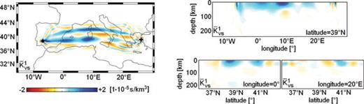
We consider a long-period full waveform tomography for the European upper mantle that is summarized in Fig. 12. The data used in the inversion are three-component seismograms with a dominant period of 100 s, that provide a good coverage of central and northern Europe (Fig. 12, left-hand side). The inversion was based on the measurement of time- and frequency-dependent phase differences (Fichtner et al. 2008). As initial model we used the 3-D mantle structure from S20RTS (Ritsema et al. 1999) combined with the crustal model by Meier et al. (2007a,b). After three conjugate-gradient iterations we obtained the tomographic images that are shown in the centre and right panels of Fig. 12, in the form of perturbations relative to the 1-D model AK135 (Kennett et al. 1995). The achieved waveform fit and the reduction of the initial misfit by nearly 70 per cent indicate that the tomographic model is at least close to optimal.

Figure 12

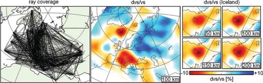
Full waveform tomography for the European upper mantle. Left-hand side: Ray coverage. Centre: Relative S wave speed perturbations at 100 km depth. Right-hand side: Zoom on the Iceland hotspot at various depth levels. The reference model is AK135 (Kennett et al. 1995).

Open in new tabDownload slide

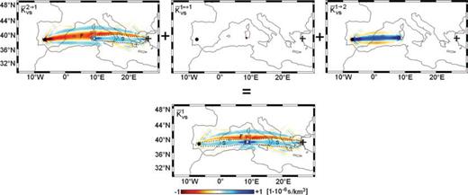
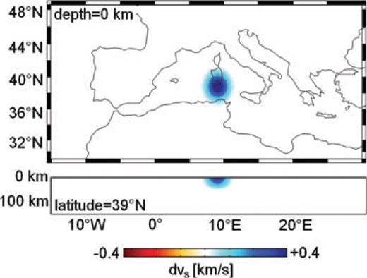
One of the most prominent features in the images is the Iceland plume (Fig. 12, right-hand side) that we choose as our model perturbation δv_S1. Horizontal slices through the isolated Iceland plume are shown in the left column of Fig. 13. Then, following the methodology from Sections 2, 3 and 5.1, we compute the corresponding approximate and full Hessian kernels, displayed in the centre and right columns of Fig. 13, respectively.

Figure 13

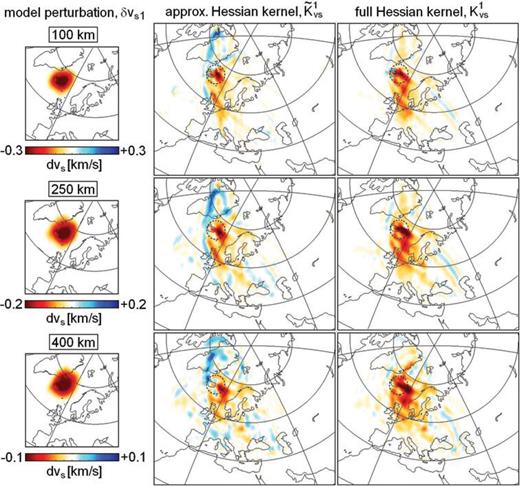
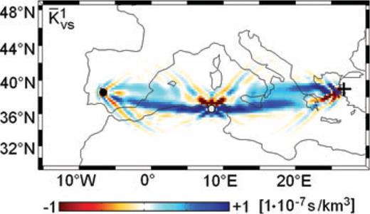
Comparison of approximate and full Hessian kernels. Left-hand side column: Slices through the Iceland plume, which serves as model perturbation δm₁= (0, 0, δv_S1). Central column: Slices through the approximate Hessian kernel . The dashed circle indicates the approximate location of the model perturbation. Right-hand side column: Slices through the full Hessian kernel . The colour scales for the approximate and full Hessian kernels are the same at each depth level.

Open in new tabDownload slide

Each of the kernels can be interpreted as the continuous representation of that row in the (approximate or full) Hessian that is associated with the Iceland plume. The volume occupied by the plume itself, and indicated by dashed circles in Fig. 13, represents the diagonal element. Off-diagonal elements correspond to volumes outside the plume.

Using this terminology, we can say that the diagonal elements of the approximate and full Hessian kernels are nearly identical at depths of around 100 km. This similarity, however, decreases steadily with increasing depth. Large differences in the off-diagonal elements, including opposite signs, are most pronounced beneath Greenland and Central Europe. This indicates that the second-order scattering contribution to the Hessian may not be negligible, even in the vicinity of the optimal model.

The Hessian kernels from Fig. 13 already provide semi-quantitative insight into where and how our image of the Iceland plume is affected by v_S structure elsewhere in the upper mantle. While structure beneath southern and eastern Europe has no effect on our perception of the plume (), its average v_S is dependent on v_S beneath northern Europe and parts of Greenland (). Based on the quadratic approximation of the misfit functional (eq. 3) we infer that increasing v_S in regions where can partly be compensated by decreasing v_S within the plume volume, and vice versa. Note that the approximate Hessian kernel would lead us to the erroneous conclusion that a decrease (increase) of v_S beneath Greenland combined with a decrease (increase) of the average plume v_S would have little effect on the misfit χ.

6 Discussion

In the previous sections, we presented an extension of the well-known adjoint method that allows us to compute the second derivatives of seismic data functionals with respect to Earth model parameters. The Hessian applied to a model perturbation, Hδm, can be represented by Hessian kernels that are similar to Fréchet kernels but also involve scattered forward and adjoint fields. This work is intended to serve as a technical prelude for the implementation of Newton's method and the development of quantitative resolution analyses in full waveform inversion. In the following paragraphs, we discuss issues related to computational aspects and to the interpretation of the Hessian kernels.

6.1 Computational requirements and the practical usefulness of Hessian kernels

The computing time required for the calculation of Hessian kernels is twice as long as for Fréchet kernels, because four instead of two wavefield simulations are needed. First, the regular wavefield u has to be modelled and stored at sufficiently many intermediate time steps. The Fréchet kernel K_m and the partial Hessian kernel K^1↔1_m can be computed during the adjoint simulation from the interaction of u and the adjoint field u^†. Two additional simulations are then needed for the perturbed regular and adjoint fields, u(m+νδm₁) and u^†(m+νδm₁), that enter the finite-difference approximations for δ₁u and δ₁u^†, respectively (eqs 93 and 94).

The comparatively high numerical costs involved in the computation of Hδm₁≡K¹_m naturally constrain the practical usefulness of the Hessian kernels. The competitiveness of Newton's method in particular will depend critically on the development of efficient algorithms that yield good approximate solutions of Newton's eq. (2) with as few evaluations of Hδm as possible. At least for 1-D full waveform inversion, a full Newton method has already proven efficient (Santosa & Symes 1988; Pratt et al. 1998).

When second derivatives are used for resolution analysis, then we are in a more favourable situation. This is because the Hessian need not be inverted to obtain a quadratic approximation of the misfit functional χ (eq. 3). The second-order expansion of χ about the optimal model already provides invaluable information about resolution and trade-offs. By choosing model perturbations δm to coincide with well-defined geological objects, the Hessian kernel formalism can be used to quantify their effect on the misfit as well as mutual dependencies (Fichtner 2010). Only for a covariance analysis sensu stricto, the inverse Hessian needs to be approximated iteratively.

6.2 Inversion for density?

Our seismically inferred knowledge on density structure is comparatively poor and almost exclusively based on the gravitational effect on long-period free oscillations (Kennett 1998; Ishii & Tromp 2001, 2004; Resovsky & Trampert 2003; Trampert et al. 2004). This is because the sensitivity of traveltime observations to density is practically zero (see for instance Fig. 10a). However, 2-D and 3-D synthetic full waveform inversions suggest that variations in ρ may also be constrained by short-period data where gravity is negligible (Köhn et al. (2010); Y. Capdeville, private communication, 2008). Our hope was therefore that density structure may have a second-order effect on traveltimes. Unfortunately, this does not seem to be the case (Figs 10b and d).

While one may argue that traveltime is not an adequate measurement to detect density variations, the scattering characteristics shown in Fig. 11 suggest that the invisibility of ρ is a more general phenomenon, at least in a transmission tomography setting. Modifications of the measurement will affect the details of the adjoint field. Yet, the scattering direction of the regular and adjoint fields from a pure density perturbation with δv_S=δv_P= 0 will remain to be opposite to the respective incidence directions. It follows that the second derivatives of any transmission tomography data functional with respect to density are small, provided that the Earth model is parameterized in terms of v_P, v_S and ρ. Changing the parameterization for instance to m= (κ, μ, ρ), will cause the density derivatives to become alive, though at the expense of substantial trade-offs between the parameters.

6.3 Full Hessian versus approximate Hessian

As we have seen in Section 5, the approximate Hessian can differ substantially from the full Hessian H, even when the model is close to optimal. The differences include sign changes and are most pronounced in the off-diagonal elements.

The explanation for the discrepancy between and H is contained in eq. (6), and it has two components. (1) The inherent non-linearity of the phase difference measurements and (2) The remaining waveform misfit that is non-zero despite the near-optimality of the model. Both factors appear to be very general because realistic misfits are never zero, and because any measurement has a non-linear contribution. Therefore, we hypothesise that the approximate and full Hessians will be different in other applications as well. This conjecture is supported by the results of Santosa & Symes (1988), who conducted 1-D synthetic waveform inversions.

The extent to which the difference between and H is practically relevant, depends strongly on the particular application. The approximate Hessian is likely to be more efficient when only the diagonal elements are used to pre-condition a descent direction within an iterative optimization scheme. However, in Newton-like methods that include the off-diagonal elements, the full Hessian may effectively lead to faster convergence. To the best of our knowledge, there is so far no experience concerning this issue. A quantitative comparison between conjugate-gradient (e.g. Mora 1987, 1988; Tape et al. 2007; Fichtner et al. 2009), quasi-Newton (e.g. Liu & Nocedal 1989; Pratt et al. 1998; Epanomeritakis et al. 2008; Brossier et al. 2009) and full Newton methods for realistic large-scale problems remains to be done.

In the context of resolution analysis, the full Hessian should be used because the approximate Hessian can lead to erroneous inferences concerning trade-offs between model parameters, as we have seen in the example from Fig. 13. Only the full Hessian allows us to correctly account for the effect of non-linearity on model resolution.

6.4 Amplitude of traveltime Hessian kernels

Fréchet kernels describe the first-order effect of structure on the measurement. For instance, a positive v_P anomaly placed within the first Fresnel zone of the Fréchet kernel in Fig. 10(a) decreases the P wave traveltime shift T because the synthetic P wave arrives earlier. The influence of the second-order effect is less clear because the Hessian kernels contain both strong negative and positive contributions. In any case, the physical relevance of the second-order effect of course needs to be considered relative to both the first-order effect and the unknown contributions of orders three and higher. A comparison of the Fréchet and Hessian kernels shown in Figs 3, 6 and 9 reveals, that the second-order effect on traveltimes can be nearly as large as the first-order effect, provided that the extent of the heterogeneity is sufficiently large. From our experience, however, we know that traveltime is quasi-linearly related to large-scale Earth structure (e.g. Tong et al. 1998). This suggests that the cumulative contribution of all higher-order terms may to some extent compensate for the non-linearity that the second derivatives appear to suggest.

7 Conclusions

We presented an extension of the well-known adjoint method to the computation of the Hessian applied to a model perturbation. The calculations involve the forward wavefield and the adjoint wavefield, as well as their scattered versions. Our approach naturally leads to the concept of Hessian kernels that can be interpreted as the continuous representation of rows (or columns) in the discrete Hessian matrix. The Hessian kernels appear as the superposition of (1) a first-order influence zone that represents the approximate Hessian and (2) second-order influence zones that represent second-order scattering. The Hessian kernels can be represented in terms of Fréchet kernels, which allows for their easy computation using codes with pre-existing adjoint capabilities.

In a series of examples, we examined second-order effects on finite-frequency traveltimes of both surface and body waves. From this we draw the following conclusions: (1) The second-order effect is relevant only when heterogeneities are located within the first Fresnel zone. This is consistent with ray-theory. (2) Second-order scattering that involves heterogeneities of different nature (e.g. v_P and v_S perturbations) appears to be inefficient, at least for P waves. (3) Second derivatives of any data functional with respect to density are nearly zero, provided that the model is parameterized in terms of density and seismic wave speeds. This result can be explained with the backward-scattering from density perturbations.

Based on a realistic full waveform tomography for European upper-mantle structure, we have shown that significant differences exist between the approximate Hessian and the full Hessian, even in the vicinity of the optimal model. These differences are largest for the off-diagonal elements, and most relevant in resolution and trade-off analysis.

Acknowledgments

First and most of all we would like to thank Theo van Zessen for maintaining the HPC cluster at the Department of Earth Sciences at Utrecht University. Furthermore, we are grateful to Christian Böhm for many vivid discussions on non-linear optimization and the computation of the Hessian for seismic observables. Insightful comments by Brian Kennett, Guust Nolet, Jeroen Ritsema, Qinya Liu, Moritz Bernauer and two anonymous reviewers helped us to improve the manuscript substantially. The numerical simulations presented in this paper were performed on the HPC system HUYGENS, and funded by NCF/NWO under grant SH-161-09.

Appendix

Appendix A: Comparison with the Discrete Adjoint Method

The discrete adjoint method is a special case of the more general continuous adjoint method, applied to physical systems that are governed by algebraic equations. These systems can be either inherently discrete, or they can be the result of a discretization process. In this section, we establish close links between the continuous adjoint method as presented in Section 2 and the discrete adjoint method as it is commonly used for 2-D full waveform tomography in the frequency domain (e.g. Dessa et al. 2004; Bleibinhaus et al. 2007, 2009; Smithyman et al. 2009). Our development is slightly more general than the one presented by Pratt et al. (1998) and Pratt (1999) because it does not rely on a least-squares misfit functional.

1 A First derivatives

We start with the generic form of the space-discretized wave equation in the frequency-domain

(A1)

where M, K and represent the mass matrix, the stiffness matrix and a discrete version of the seismic displacement field. The variables ω and are the angular frequency and the discrete external force density. Defining the impedance matrix L(ω) =−ω²M+K, we can rewrite eq. (A1) in the form of a simple matrix-vector equation

(A2)

The matrix L now contains all the structural information of the Earth model, that is, L=L(m). Furthermore, we assume that the model space is finite-dimensional, so that any model can be written in the form of a vector with n < ∞ components

(A3)

We are interested in the partial derivatives of the data functional with respect to the model parameters m_i

(A4)

To eliminate from eq. (A4) we differentiate the discrete wave eq. (A2) with respect to m_i

(A5)

The appearance of the inverse L⁻¹ in eq. (A5) is purely symbolic. It does not have to be computed in practice. Substituting eq. (A5) into eq. (A4) yields

(A6)

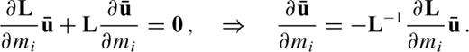
We now define the discrete adjoint wavefield as the solution of the adjoint equation

(A7)

Clearly, eq. (A7) corresponds to the adjoint equation that we found in the continuous case (eq. 21). With the help of the discrete adjoint field we can now obtain a simple expression for

(A8)

As in the continuous case, the computation of the partial derivatives of χ reduces to the solution of the adjoint eq. (A7) with an adjoint source determined by the data functional. The continuous counterpart of eq. (A8) is (eq. 22).

2 A Second derivatives

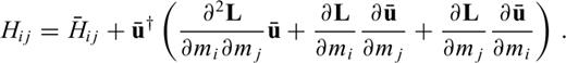
Following the recipe from the previous section, we can derive an expression for the second derivative of χ in terms of the adjoint field , as defined in eq. (A7). Differentiating χ first with respect to m_i and then with respect to m_j gives

(A9)

where the components of the approximate Hessian are defined as

(A10)

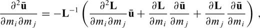
In contrast to the full Hessian, H_ij, the approximate Hessian merely involves first derivatives which makes its practical computation via the standard adjoint method comparatively straightforward. To eliminate the second derivative from eq. (A9), we differentiate the forward problem (A2) twice

(A11)

The rearrangement of eq. (A11) provides an explicit expression for ,

(A12)

that we substitute into eq. (A9)

(A13)

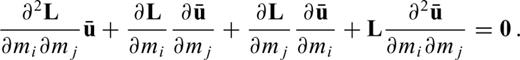
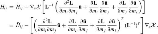
Again defining the adjoint field as the solution of

(A14)

yields the desired formula for H_ij that is free of the explicit inverse of L and that does not contain second derivatives of

(A15)

Eq. (A15) is the discrete analogue of the Hessian for time- and space-continuous problems (eq. 44).

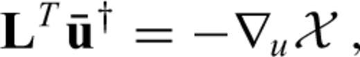
References