Shallow structure of Deception Island, Antarctica, from correlations of ambient seismic noise on a set of dense seismic arrays

Summary

1 Introduction

Recent theoretical advances have shown that under the assumption of evenly distributed sources of noise, the Green's function between two points can be estimated from the cross-correlation of records obtained at these sites (Weaver & Lobkis 2001a,b, 2004; Derode et al. 2003; Snieder 2004; Wapenaar 2004; Larose et al. 2005; Sánchez-Sesma et al. 2006, 2008; Pérez-Ruiz et al. 2008; Colin de Verdière 2009).

The results of using diffuse seismic wavefields to extract the Green's function have also been substantiated using earthquake coda waves (Campillo & Paul 2003; Paul et al. 2005) and ambient seismic noise for both surface waves (e.g. Shapiro & Campillo 2004; Sabra et al. 2005a) and body waves (Roux et al. 2005). The extraction of the Green's function from correlations has been applied in other fields such as helioseismology (Rickett & Claerbout 1999), ultrasonics (Weaver & Lobkis 2004) and acoustics (Sabra et al. 2005a). The historical development of this technique in the context of seismic interferometry is described in chapter 1 of Schuster (2009).

Traveltime measurements of Rayleigh waves reconstructed from the seismic noise have been used to produce high resolution images on regional (Sabra et al. 2005b; Shapiro et al. 2005; Kang & Shin 2006; Yao et al. 2006; Lin et al. 2007; Moschetti et al. 2007) and continental (Yang et al. 2007; Bensen et al. 2008) scales. The applicability of the method at higher and lower periods has also been analysed. Bensen et al. (2008), Yang et al. (2007) and Ruigrok . (2008) obtained results for periods >50 s, whereas Chávez-García & Luzón (2005) and Picozzi . (2009) used cross-correlations in periods <1 s. Most of these studies were performed in time domain by means of measurements of the group velocity of Rayleigh waves. Such dispersion curves can be used to construct velocity maps that usually exhibit striking correlations with the observed geological structures. However, few authors to date have used the empirical Green's functions obtained from cross-correlations to estimate Rayleigh-wave phase velocities. Of these, the regional scale tomographic maps of southeastern Tibet (Yao et al. 2006), western United States (Lin et al. 2008) and Costa Rica and Nicaragua (Harmon et al. 2008) are particularly noteworthy. As suggested by Lin . (2008), phase velocity measurements are preferable to group velocities because dispersion curves for group velocity can be calculated easily from those for phase velocity.

In this paper, we computed phase velocities of Rayleigh waves from ambient noise records obtained at several seismic arrays deployed at Deception Island volcano, Antarctica, during the period 2003–2005. We obtained results for frequencies of up to about 9 Hz, and used them to estimate S-wave velocity profiles for the locations of these arrays. We begin by describing the site and the data set used in this study. We then go on to explain briefly the fundamentals behind the extraction of the imaginary part of the Green's function and the hypotheses to connect it with the spatial autocorrelation function defined by Aki (1957). Afterwards, the entire procedure to obtain both the phase velocities of Rayleigh waves and the global S-wave velocity model is shown for a representative array. Finally, we present the application of the method to the seismic noise recorded by all the seismic arrays. The results allowed us to obtain an approximate vertical section of the shallow velocity structure along the inner coastline of Deception Island.

2 The Site

Deception Island is a stratovolcano located in the Bransfield Strait, between the Antarctic Peninsula and the South Shetland Islands (Fig. 1). The basal diameter of the island is 30 km and it rises 1400 m from the seafloor to a maximum height of 540 m above sea level. The 15-km-diameter island is horseshoe-shaped and has a flooded caldera (Port Foster) with dimensions of about 6 × 10 km and a maximum depth of 190 m. Deception Island is the most active of all the volcanoes in the South Shetland Islands, having erupted at least six times since it was first visited 160 yr ago (Newhall & Dzurisin 1988; González Ferrán 1995). All recent eruptions were relatively small in volume and occurred at locations near the coast of the inner bay. There were three eruptions between 1967 and 1970 along the north and east sectors of the island, all of which were observed directly and are well documented (Baker et al. 1969, 1975; Smellie 1988).

Figure 1

(Upper left-hand side) Location of Deception Island in the Bransfield Strait, between the South Shetland Islands and the Antarctic Peninsula. (Bottom left-hand side) Sketch of the main volcanic features of Deception Island. (Right-hand side) Locations and configurations of the seismic arrays used in this work. Sensors are represented by triangles. The three inserted panels detail the station distributions at sites G, D and H.

Open in new tabDownload slide

Glaciers cover a large portion of Deception Island, especially the Mount Pond and Mount Kirkwood slopes, in the east and south, respectively. Young pyroclastic deposits and sediments cover most of the rest, except for a few sites where older rocks are exposed (e.g. Martí & Baraldo 1990; Smellie 2001).

Evidence of present-day volcanic activity at Deception Island includes fumarolic emissions, hydrothermal activity, resurgence of the northern floor of Port Foster and both volcano-tectonic and long-period seismicity (Ortiz et al. 1992, 1997; Rey et al. 1995; Cooper et al. 1998; Ibáñez et al. 2000, 2003a,b).

Fumarole fields and hot springs with temperatures generally below 110 °C encircle Port Foster (Smellie 1990; Ortiz et al. 1992; Villegas et al. 1997; Caselli et al. 2002). Fumarole Bay in the W sector of Port Foster takes its name from the active fumaroles in the area. Fumarole temperatures and compositions are not constant and have displayed some correlation with the level of seismo-volcanic activity (Caselli et al. 2004). Hot springs are common in the northern and eastern sectors of Deception Island, although they are especially active in Pendulum Cove and Whalers Bay (see Fig. 1).

The seismic activity of Deception Island has been monitored since 1986 by different research teams, under the framework of the Spanish Antarctic Program. All surveys took place during the Antarctic summer, and used several seismometer configurations including seismic networks and small-aperture seismic arrays. These surveys detected both long-period and volcano-tectonic seismicity (see e.g. Chouet 1996). Long-period seismicity, probably related to water/steam-magma interactions, was recorded and analysed using array techniques (Almendros et al. 1997, 1999; Ibáñez et al. 2000). This seismicity was very common between 1994 and 1999, but in recent years has decreased sharply. Volcano-tectonic earthquakes generally occur in swarms. Two were reported in 1992 and 1999 (Ortiz et al. 1997; Ibáñez et al. 2003a), although the lack of a permanent network prevents us to exclude other occurrences. These swarms contained small earthquakes, with magnitudes of below 3. They occurred mostly along fracture systems trending NE–SW (Vila et al. 1992; Ibáñez et al. 2003a), but with a variety of source mechanisms reflecting a complex relationship with subsurface magma motions (Ibáñez et al. 2003b; Carmona et al. 2010).

3 Instruments

We used records of ambient seismic noise obtained in eight seismic arrays deployed along the inner coast of Deception Island (Fig. 1) at different periods between 2003 and 2005. Array D was installed from 2003 December to 2004 February, during the 2003–2004 Spanish Antarctic survey, to monitor the seismo-volcanic activity of Deception Island. The remaining arrays (M, E, F, J, G, L and H) were deployed during a two-week active-source seismic tomography experiment that took place in 2005 January (Zandomeneghi et al. 2009).

All instruments were Mark-L28 seismometers with a natural frequency of 4.5 Hz. Their responses where electronically extended to achieve a flat velocity response down to 1 Hz. Sampling was performed at 100 sps using 12-channel, 24-bit data acquisition systems working in continuous mode. Seismic data were stored on a local hard disk. A GPS receiver was used to synchronize the internal clock every second [see Abril (2007), for a complete description of the recording systems].

Each array included up to 12 vertical seismometers and one three-component sensor, connected by cable to the acquisition system. Array configurations varied according to logistic difficulties, access limitations imposed by the topography and the specific objectives of the experiment. At some sites, the sensors were distributed randomly, while at others they followed a regular pattern. Array apertures ranged between 0.3 and 1.3 km. Station coordinates were measured with a laser theodolite with respect to a reference benchmark, whose absolute geographic coordinates were obtained using GPS.

4 Method

4.1 Connection between the Green's function obtained from the cross-correlation of noise and the coherence function

As has been demonstrated (see e.g. Sánchez-Sesma & Campillo 2006; Sánchez-Sesma et al. 2006, 2008), if a diffuse harmonic displacement vector field u_i(x, ω) is established within an elastic medium, the average cross-correlation of such motions at points x and y is proportional to the imaginary part of the elastodynamic Green's function between both locations, that is

1

where ω is the circular frequency, and K a positive constant. In noise-based imaging, the surface wave dispersion characteristics are commonly used since the Green's function between points at surface is dominated by surface waves, and because the background seismic noise consists mainly of these waves (see e.g. Friedrich et al. 1998; Ekström 2001). In the case of horizontally layered media, the Green's function for vertical displacement on the surface, due to Rayleigh waves generated by a surface vertical point source can be expressed as

2

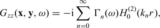
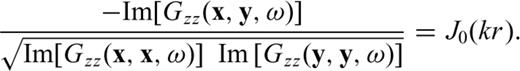
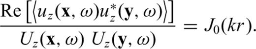
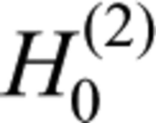where Γ_n is a positive real quantity depending on the Rayleigh-waves medium response and on the ellipticity of the n-th surface wave mode (see e.g. Haskell 1953; Harkrider 1964); represents the Hankel function of second kind and zeroth order; k_n is the n-mode Rayleigh wavenumber; i the imaginary unit and r is the distance between points x (receiver) and y (source). If we consider that there is a predominant mode for Rayleigh-wave propagation in the frequency range of interest, then the imaginary part of the elastodynamic Green's function between the two locations is precisely

3

where J₀ is the Bessel function of first kind and order zero. It should be noted that the imaginary part of the Green's function is still finite when x=y, since the singularity is restricted to its real part. As can be observed here and as was stated previously by Sánchez-Sesma . (2009), the imaginary part of the Green's function at the source itself exhibits intrinsic properties of the site. In particular, it represents the rate of energy injected by the unit harmonic load at that point in the vertical direction (see e.g. Perton et al. 2009; Snieder et al. 2009). Since Im[G_zz(x,x,ω)] equals Im[G_zz(y,y,ω)] for x≠y in any horizontally layered medium excited with a diffusive wavefield, we can use both quantities to normalize the imaginary part of the Green's function between the locations x and y as

4

Finally, using the last equation together with eq. (1), it is possible to write a compact expression for the normalized cross-correlation in the frequency domain in terms of the coherence function

5

This result is essentially the same as that obtained in the pioneering work by Aki (1957) for the spatial autocorrelation coefficient, and can be used to obtain the phase velocity for a given frequency and distance. This expression of the coherence between signals u_z(x, t) and u_z(y, t) has also been used as the basis of the two-station spatial autocorrelation method (SPAC, see e.g. Morikawa et al. 2004; Chávez-García et al. 2005). An experimental relationship between the Green's function extracted from the cross-correlation of noise and Aki's SPAC was also obtained by Chávez-García & Luzón (2005), whereas the first theoretical connection between both concepts in an elastic, isotropic and homogeneous medium was introduced by Sánchez-Sesma & Campillo (2006). The consistency of the SPAC with seismic interferometry was studied in the recent work of Yokoi & Margaryan (2008), who concluded that both methods are consistent for azimuthally isotropic wavefields, whereas azimuthal averaging is needed for an azimuth-dependent wavefield. They proposed using a triangular array to avoid this problem in practical cases. Recently, Prieto . (2009) showed experimentally the consistency between time and frequency domain methods for extracting Green's functions.

From the theoretical point of view, the numerator on the left-hand side of eq. (5) will be real. In fact, Asten (2006) and Margayan . (2009) use the imaginary part of the coherence function as a quality indicator of the performance of the SPAC technique, relating the lack of wavefield isotropy with the non-zero imaginary part. In isotropic wavefields, the cross-correlograms will be symmetric in the time domain (i.e. the ‘causal’ and ‘anticausal’ signals corresponding to waves propagating in opposite directions between the stations will be symmetric). However, in real problems the cross-correlograms are not completely symmetric and a process of averaging is usually needed to obtain a single ‘symmetric signal’ (see e.g. Bensen et al. 2008). It can be shown that this symmetrization process in time domain is equivalent to taking the real part of the coherence in frequency domain. Applying this to the left-hand side of eq. (5) it reads

6

Note that to preserve the applicability of eq. (6) the hypotheses considered above have to be satisfied in the frequency range of interest: (i) the existence of a predominant mode for Rayleigh-wave propagation, and (ii) the consideration of a horizontally layered medium which implies that U_z(x, ω) ≈ U_z(y, ω) in eq. (6). Both hypotheses are reasonable and commonly assumed in velocity structure inversions based on surface waves.

4.2 Computation of the S-wave velocity model: the example of site G

In this section we use site G as an example to explain the procedure used to estimate all the S-wave velocity models in Deception Island.

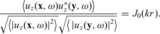
We started by selecting several hours of noise recorded simultaneously by two stations of the array. We divided these records into a set of 80 per cent overlapping windows of 20 s, which gave us in our subsequent treatment a frequency resolution of 0.05 Hz. A Hanning taper was applied to the time windows on 10 per cent of their lengths. Then, their Fourier spectra were obtained by using the discrete Fourier transform (DFT) algorithm. These spectra were slightly smoothed in amplitude using a 0.3 Hz moving window. Finally, we computed the average normalized cross-correlations (or the average coherence) following eq. (6). We applied this procedure to several hours of noise, observing that the frequency-dependent curve obtained from eq. (6) did not change significantly when more than 5 hr of noise were used. This method was repeated for all station pairs deployed at the site and results are shown in Fig. 2. The different panels were sorted with increasing distance between sensors. It can be seen that the frequency of the first zero-crossing of these curves decreases with increasing distance.

Figure 2

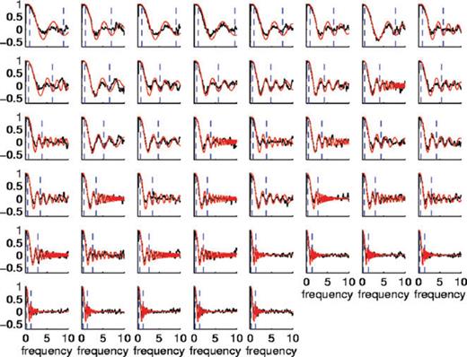
Average normalized cross-correlations (black lines) as a function of frequency (in Hertz) for all possible stations pairs within array G. The red lines show the best-fit for each station pair. The range of frequencies used for the fit is marked by blue vertical dashed lines. The panels are sorted from left to right and from top to bottom by increasing station distance.

Open in new tabDownload slide

Using an iterative least-squares algorithm, we fitted these experimental curves to zeroth-order Bessel functions, independently for each pair of stations. The argument of the Bessel functions was derived from substitution in (6) of the generic smooth dispersion relationship (Chouet et al. 1998)

7

where f is the frequency, and A, a and b are constants. The frequency range used was such that the argument of the Bessel function J₀ runs from 0.4 to 10. The lower limit, in which the Bessel function has a value close to 1, is the same proposed by Henstridge (1979) for the Aki (1957) method. For the upper limit of the argument, the Bessel function reaches its second minimum. This minimum is usually well developed in the experimental curves, and therefore is used in the fitting process. Note that the frequency of the second minimum depends also on the distance r between the stations. Fig. 2 shows the coherence curves obtained with the noise data (in black) together with the fitted curves (in red) for each pair of stations at site G. In each case, the frequency range used in the fit is marked with two blue vertical dashed lines.

A global dispersion curve was constructed for each site as the mean value of the phase velocities obtained from the pairs of stations. For any frequency, we required the contribution of, at least, two station pairs to obtain its mean phase velocity and its corresponding standard deviation. Fig. 3 shows the calculated dispersion curve for the example site G (solid line) together with the standard deviation (dashed lines). Phase velocity ranges from about 2 km s⁻¹ at lower frequencies to ∼350 m s⁻¹ at frequencies above 4 Hz. The small standard deviation implies that all the azimuths defined by the pairs of stations lead to very similar phase velocities. This is consistent with the initial hypothesis of elastic medium with 1-D local response illuminated with a diffuse wavefield.

Figure 3

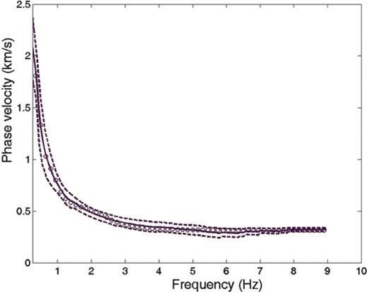
Experimental average phase–velocity dispersion curve for Rayleigh waves (solid line) obtained for site G. The standard deviation is shown with dashed lines. Open circles represent the dispersion curve computed for the best-fitting S-wave velocity model obtained in the inversion procedure.

Open in new tabDownload slide

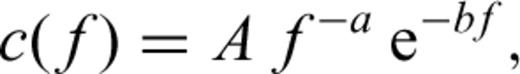
Once we had a reliable phase velocity dispersion curve, we inverted it to obtain the S-wave velocities for a horizontally layered model, assuming dominance of the fundamental mode of Rayleigh waves. For this purpose we have developed a parallel computer program based on linearized least-squares inversion codes (Herrmann 1987) that performs many simultaneous local optimizations from a set of randomly generated initial models. This procedure circumvents the need for the initial velocity model required by the Herrmann's codes, which to some extent, determines the final model resulting from the inversion. Additional constraints obtained from other methods are often useful to preserve the uniqueness of the resulting velocity model. Unfortunately, such constraints cannot be clearly stated in our case and some kind of intensive search in the model space (such as that described above) is required.

The exact procedure for inversion was implemented as follows. First, we constructed a preliminary subsurface model for Deception Island (see Table 1) as a combination of the 1-D models proposed by Ibáñez et al. (2000) and Saccorotti et al. (2001). Our model was composed of three layers and a half-space. Properties of Layer 1 were obtained by averaging the first two layers of the local model obtained by Saccorotti et al. (2001) for the Obsidianas Beach site in Deception Island. Layers 2, 3 and the half-space had the same properties as layers 2–4 of the regional model used by Ibáñez et al. (2000) for Deception Island. We then constructed 1000 initial models by introducing random variations of up to ±50 per cent in thicknesses and S-wave velocities of the layers of this preliminary model. Finally, we applied Herrmann's codes for each of these 1000 initial models to obtain their respective converging final results, and extract the best one among these final models. The damping factor was decremented down to 0.1 in the last iterations of the inversion (see e.g. Okada 2003; Pei 2007).

Table 1

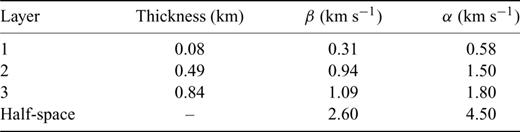
Preliminary velocity model considered in this work. The model was constructed from a combination of the 1-D models proposed by Ibáñez. (2000) and Saccorotti et al. (2001) (see text for explanations). α:-P-wave velocity; β:-S-wave velocity.

Open in new tabDownload slide

The phase velocity dispersion curve for the final model of site G is shown in Fig. 3 with open circles. It can be observed that the fit between the empirical phase velocities and the dispersion curve derived from the final model is very good.

Fig. 4 shows the final model obtained for site G, together with the resolving kernels for the inversion procedure. These kernels indicate whether a layer can be resolved by the procedure or not. For any well-resolved layer, a single peak of significant amplitude is displayed at the depth of the layer. In this case, the resolving kernels for the G model suggest that it can be considered well resolved except for the half-space, where the corresponding kernel shows a very low value at its depth.

Figure 4

(Left-hand side) S-wave velocity structure obtained for array G with their uncertainties. (Right-hand side) Resolving kernels for each layer. Errors and resolving kernels were calculated with a damping factor of 0.1. Note that the S velocity of the half-space, which cannot be considered well resolved from its resolving kernel, is shown with a discontinuous line.

Open in new tabDownload slide

5 Results for All the Sites

We applied the method described earlier to obtain subsurface models for the eight sites selected at Deception Island. In the first stage of our investigation, we confirmed that the set of curves for all the station pairs at each site was self-consistent (in the sense discussed for Fig. 2). That is, the frequency of the zero-crossings of these curves should decrease with increasing distance between sensors. All the sites followed this pattern, except for site F located in the NW sector of Port Foster. Correlations at site F indicated that the velocity structure may change across the area covered by the seismic stations.

To check if the required hypotheses were satisfied at site F, we compared the spectra calculated at different stations. In a horizontally layered medium, these functions should be the same regardless of the station used for its calculation. In fact, U_z displays a similar shape for the different seismometers for most of the sites, with peaks around common frequencies and small differences in their amplitudes (factors below 2.5). For example, we show U_z for the stations deployed at site J in Fig. 5(a). The shapes are similar and all of them peak at about 0.7 Hz. However, site F does not show the same regular pattern (Fig. 5b). Based on the shape of U_z we can define two separated subsets of stations, which we shall call F1 and F2 (Fig. 1). The subarray F1 (made up of sensors 5, 6 and 7) has a common peak around 0.5 Hz, whereas subarray F2 (sensors 8, 9 and 11) presents a peak at about 0.8 Hz. The remaining sensors (1, 4 and 10) have peaks at intermediate frequencies, possibly indicating a transition zone. Since the structures under F1 and F2 are obviously different, we will analyse the F1 and F2 stations separately to produce a total of nine (instead of eight) velocity models.

Figure 5

U_z functions (see eq. 6) obtained from seismic noise recorded at the vertical-component channels of arrays J (a) and F (b). The insets show the relative positions of the stations, on the same scale (see Fig. 1).

Open in new tabDownload slide

The dispersion curves computed for the all the sites are presented in Fig. 6 for comparison purposes. Estimated phase velocities range from ∼0.25 to 2.4 km s⁻¹. The curves span different frequency intervals related to the array configurations. The high-frequency limits of the dispersion curves range from 1.5 to 3 Hz for the coarsest arrays (M, F1, F2 and J) to 9 Hz for the densest arrays (G and H). Each dispersion curve is different from the others, showing that each site has different subsurface conditions. However, we also observed that some sites had common features. For example, all the sites show phase velocities concentrated between 450 and 650 m s⁻¹, approximately, around 2 Hz, except for M and F1. The highest velocity at that frequency (∼850 m s⁻¹) was for the M site, while the lowest (∼450 m s⁻¹) was for site H. However, the dispersion curve for the F2 subarray reaches 400 m s⁻¹ at about 1.5 Hz, and its shape suggests that this could be the slowest site of all.

Figure 6

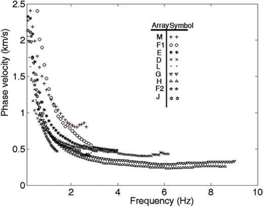
Dispersion curves of Rayleigh waves obtained for the nine sites investigated in this study.

Open in new tabDownload slide

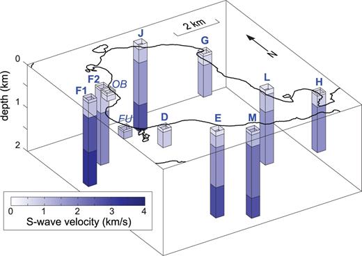
Once we had the average dispersion curves for each site, we estimated the respective velocity models by using the procedure described above. The results were a set of 1-D S-wave velocity models spatially distributed along the inner coastline of Deception Island. Fig. 7 shows the details of the individual models, and Fig. 8 shows a spatial view of the estimated velocity structures at the different sites.

Figure 7

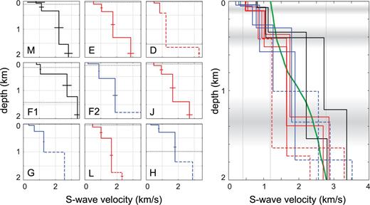
S-wave velocity models obtained for the nine sites investigated in this work. The uncertainties in the layer velocities are indicated by horizontal segments. Poorly constrained layers are shown with dashed lines. Dotted lines show the penetration depths estimated as 1/3 of the largest and smallest Rayleigh wavelengths in the experimental dispersion curve. The right panel shows all models in the same plot, to make comparison easier. The green line is the average model for the Bransfield Strait crust near Deception Island (modified from Christesson et al. 2003). The grey bands indicate common depth ranges of layer boundaries. Colours identify sites with similar characteristics (see text for explanations).

Open in new tabDownload slide

Figure 8

Sketch of the S-wave velocity structures derived at the sites along the inner coastline of Deception Island. We show only well-constrained layers. All column tops are at sea level. FU and OB indicate the models derived by Saccorotti et al. (2001), shown for comparison.

Open in new tabDownload slide

The derived models reflect the variability already observed in the dispersion curves. There are some common characteristics, but also several differences pointing out to the heterogeneity of the shallow structure in Deception Island volcano. We were able to resolve four layers at most sites, except for D (two layers), G, L and H (three layers). Well-constrained model velocities range from ∼200 m s⁻¹ for the shallowest layer under site F2 to 3.4 km s⁻¹ for the deepest layer under site F1. The first layer is a soft surface layer (layer 1) with S-wave velocities of between 200 and 800 m s⁻¹ extending down to ∼100 m. This layer is thinner (∼50 m) and slower (∼200–300 m s⁻¹) for sites F2, G and H (blue lines in Fig. 7). By contrast, the shallowest layers of the M and F1 models (in black in Fig. 7) are much faster (∼800 m s⁻¹). However, in the cases of arrays M, F1 and F2 the calculated dispersion curves do not reach very high frequencies (see Fig. 6) and these results corresponding to thin shallow layers have to be interpreted with a pinch of salt. Next, we detect an intermediate layer (layer 2) with S-wave velocities between 0.7 and 1.1 km s⁻¹, extending down to a depth of about 400 m. Again, the lowest velocities are found at sites G and H, while the highest velocities correspond to sites M and F1. These layers 1 and 2 seem to be found everywhere around Port Foster, with slightly different velocities and thicknesses. However, structures below ∼400 m are more diverse. We found a deeper layer (layer 3) with a thickness of about 1 km, characterized by S-wave velocities in the broad range between 1.3 and 2.8 km s⁻¹. The lower boundary of this layer is not well resolved at sites F2, G, L and H. At sites M, E, F1 and J it extends down to 1.2–1.5 km. Model G displays the lowest velocity of about 1.3 km s⁻¹, and once again M and F1 are the fastest with values of 2.2 and 2.7 km s⁻¹, respectively. The remaining models (E, F2, L and H) range between 1.6 and 1.9 km s⁻¹. Finally, the velocities of the underlying half-spaces (layer 4) range between 2.7 and 2.9 km s⁻¹ for sites M, E and J. In the case of site F1, layer 4 reaches 3.4 km s⁻¹. However, we feel that this result is not well constrained. This value is about 40 per cent larger than the largest phase velocity estimated for this site, corresponding to a frequency of 0.5 Hz. At these long wavelengths, the phase velocity should be closer to the half-space velocity. We assume that we cannot investigate adequately depths beyond one-third of the largest wavelength in our dispersion curve (dotted lines in Fig. 7). Layer 4 at site F1 is mostly below this limit, and thus remains largely unconstrained.

The F1 model is generally faster than the rest of the models. This reveals that the stations at this site were deployed on a hard structure. Note, for example, that velocities of 2.7 km s⁻¹ are already found at just 400 m (layer 3). This fact is compatible with the dispersion curve for array F1 (Fig. 6), which has the highest phase velocities at low frequencies. The M model is similar to F1 at shallow depths, but slower below 400 m. In both M and F1 the uncertainties associated with the velocity estimates are relatively large up to about 0.5 km s⁻¹.

6 Discussion

Our results are consistent with velocity models estimated for Deception Island and surrounding areas with different techniques (e.g. Grad et al. 1992; Christesson et al. 2003; Ben-Zvi et al. 2009; Zandomeneghi et al. 2009). These models assign P-wave velocities between 2 and 5 km s⁻¹ for the shallowest 2 km of the crust. Assuming a Poisson ratio of 0.25, these values represent an S-wave velocity range of ∼1.2–2.8 km s⁻¹. For example, Fig. 7 includes an average model obtained from Christesson . (2003), who investigated the velocity structure of the Bransfield Strait area. This model reproduces the general trend of the velocity models obtained here. However, there are two important differences. First, our models consistently show S-wave velocities lower than the Christesson . (2003) average for the first half kilometre. This reflects the fact that our experiment took place on a volcanic setting made of pyroclastic deposits and loose sediments, which are characterized by low velocities of seismic waves. In this way, we obtain low S-wave velocity values for these shallow layers in comparison with the average crust of the Bransfield Strait. Secondly, there is an obvious dispersion of the results, especially at depth. This dispersion suggests a large degree of lateral heterogeneity in the velocity structure, which demonstrates the complexity of the shallow structure of Deception Island volcano.

This heterogeneity is not so evident at first sight. The morphology of Deception Island, with its circle of high walls surrounding Port Foster, suggests some degree of radial symmetry that we have not found in our results. Our instruments were deployed at the most accessible sites along the Port Foster coastline, at distances of approximately 2–4 km (Fig. 1). These sites are generally wide valleys, open beaches or relatively flat slopes. Deception Island soils are basically constituted by pyroclastic deposits of different post-caldera eruptions (Smellie et al. 2002). At some sites, especially at sites F, J, L and H, an undifferentiated sedimentary layer (alluvium, beach and scree deposits) of variable importance can also be found. Apparently, the shallow geology of the array sites does not reveal significant differences.

In spite of this apparent uniformity, our results show important differences even for neighbouring sites. For example, the shallowmost layers of the F2, G and H models display very low S-wave velocities (Figs 7 and 8). These layers are not only slower but also thinner than in the remaining models. Interestingly, the areas where these arrays were located are characterized by the presence of vigorous hydrothermal activity (see Fig. 1). In particular, the G and H sites located at Pendulum Cove and Whalers Bay, respectively, show continuous emanations of water vapour and shallow circulation of hot water. Hydrothermal fluids and alterations may be responsible for the low S-wave velocities observed at these sites.

Model M, by contrast, has a high-velocity surficial layer. Since there are large uncertainties in this layer we have to be cautious with the interpretation. However, a fast shallow layer is not an unreasonable feature. The M site includes areas covered by recent lava flows, and lacks the presence of craters and/or cinder cones (Smellie et al. 2002). Such structures are definitely common in surrounding areas such as the E site, just ∼1.5 km away. These differences point to a lateral velocity contrast and a fast shallow structure of the M site. However, there is also a possibility that the fast layer could be an artefact due to the restrictions imposed by the dispersion curve. In other words, one of the hypotheses of our method requires that Rayleigh waves be dominated by the fundamental mode. However, the ascending high-frequency tail of the dispersion curve for site M (Fig. 6) might indicate the presence of a higher mode. We believe that the differences in the shallow geology described earlier support the former explanation and rule out the presence of higher modes, which have not been detected anywhere else.

The second layer, between the discontinuities at about 100 and 400 m (Fig. 7), is perhaps more homogeneous, with a velocity range of 0.7–1.1 km s⁻¹. This layer may correspond to more consolidated volcanic deposits and sediments from the post-caldera eruptions that took place around Port Foster. These eruptions were generally small, and affected limited areas of the island, which may have produced the differentiation we observed. Mass flow related to erosion, sedimentation and snow cycles may also be responsible for part of this differentiation. S-wave velocities maintain approximately the same order as in layer 1 (Fig. 7), which suggests that the effects described in the previous paragraph have a downward continuation and affect a thicker layer of the medium. In the case of site G, these effects might also affect layer 3, which displays the lowest resolved velocity at that depth.

Another interesting result illustrating the heterogeneity of Deception Island volcano is the very different characteristics of the velocity structures under subarrays F1 and F2 (Figs 7 and 8), which are very near each other. Array F covers a wide area extending from Cross Hill to Morature Point in N–S direction and from Obsidianas Beach to the caldera ridge in E–W direction. The F1 stations were located to the SW of this area, near the foot of the steep slopes that characterize the inner side of the caldera wall. These slopes are made of exposed pre-caldera rocks, mainly belonging to the basaltic shield formation (Smellie et al. 2002). By contrast, F2 stations were located to the NE, farther from the caldera wall. The F2 area is covered by beds of pyroclastic deposits from recent, post-caldera eruptions.

Our results show that model F1 is much faster than model F2. For example, it reaches velocities of 2.7 km s⁻¹ at a depth of just 400 m. A velocity of that order is never found in model F2, at least down to the resolved depth of ∼1.8 km. These differences suggest that the SW stations of array F were located on a particularly hard structure. The hardness of this structure may be related to the presence of pre-caldera deposits at shallow levels, as hinted by the nearby outcrops. Pre-caldera rocks are exposed at other points on Deception (e.g. Fumarole Bay, Cathedral Crags, the external coast along Kendall Terrace) and are assumed to underlie the whole island. However, the evidence shows that only the F1 stations were close enough to detect their effect on the inverted 1-D model. In the case of site F2 the velocity structure is much slower, and quite alike the models found in similar environments of the island such as sites G and H. The distance from F1 to F2 is just ∼1 km, which emphasizes the sharpness of this lateral velocity contrast.

The existence of a sharp lateral velocity contrast between the F1 and F2 sites had been suggested by previous seismological evidence. For example, Saccorotti . (2001) detected strong refractions of seismic waves in this area. They deployed two small-aperture seismic arrays. Array OB was approximately colocated with station 8 of the F2 subarray, while array FU was deployed on the coast of Fumarole Bay. They applied the SPAC method and found that the FU velocity model was faster than the OB model (see Fig. 8). They hypothesized the continuity of a fast structure related to pre-caldera rocks that extended from FU towards the NE and N along the caldera ridge. The velocity structure west of the OB array would then be comparable to the structure under the FU array, thus producing a strong lateral velocity contrast.

Results from a seismic tomography experiment performed at Deception Island in 2005 January (Zandomeneghi et al. 2009) also revealed a sharp lateral velocity contrast in the Obsidianas area. This area is cramped between the high-velocity South Shetland basement and a low-velocity magma chamber located below Port Foster. The maximum horizontal gradient in P-wave velocity observed at 1 km depth in this area is about 1 km s⁻¹ in just 1 km in E–W direction. This observation fully coincides with our results.

Another clue that may help us with the interpretation of the differences between models F1 and F2 comes from the work of Carmona et al. (2010). They investigated the geometry of the fault planes involved in the 1999 seismic series of Deception Island volcano (Ibáñez et al. 2003a) located under the northern half of Port Foster. They found that most of the active faults corresponded to subvertical planes oriented in a NW–SE direction. The abundance of NW–SE faults in the area suggests the hypothesis of a NW–SE fault under the F site at Obsidianas Beach, which would separate the F1 and F2 stations. The presence of such a fault might help understand the differences between these velocity models.

7 Conclusions

In this paper, we computed the phase velocity of Rayleigh waves from noise records obtained at several seismic stations deployed at Deception Island volcano, Antarctica, during the period 2003–2005. The technique is based on the extraction of the imaginary part of the Green's function for Rayleigh waves by means of the coherence of isotropic ambient noise, under the hypotheses of a predominant mode for Rayleigh-wave propagation and the consideration of a horizontally layered medium. These hypotheses form the basis for the connection of the average coherence of noise at two stations and the Bessel function of order zero in eq. (6). Since we are working with dense seismic arrays, we can use this method for each station pair within the array covering different azimuths. Thus, a global dispersion curve for each array site can be constructed from the mean value of the phase velocities obtained for each pair of stations.

This method was applied to all possible stations pairs within the eight seismic arrays deployed at Deception Island during the period 2003–2005. Array F was divided into two different subarrays made up of stations showing similar spectral properties. The differences between the typical spectra recorded at these subarrays suggest that the structure beneath the whole array F is far from being a horizontally layered medium. This fact seems to agree with the results of other seismic and geomorphological surveys. As a consequence, we conclude that the similarity of these spectral properties may be useful as a quality indicator for this method. This topic is currently under research.

We calculated average dispersion curves for these nine sites, and inverted their respective S-wave velocity structures. Using these results, we conclude that the shallow structure of Deception Island volcano is composed of relatively soft layers of pyroclastic deposits and sediments extending to a depth of about 400 m, with different degrees of compaction. Two layers with thicknesses of about 100 and 300 m and S-wave velocities around 0.2–0.8 and 0.7–1.1 km s⁻¹, respectively, can be differentiated. The deeper structure is highly variable in terms of wave velocities and layer depths, which indicates a laterally heterogeneous structure. Although the resolving capabilities for these layers are limited, the larger S-wave velocities in the range 1.3–2.8 km s⁻¹ indicate that they may be associated with pre-caldera structures and products.

Apart from the simplified view of the seismic structure of Deception Island described earlier, our results highlight the substantial differences between the different array sites. These variations may be spatially related to volcanic features and structures. For example, the lowest S-wave velocities are related to alterations produced by hydrothermal activity near the surface at the F2, G and H sites. By contrast, the highest velocities occur at the F1 site near the caldera border, revealing the presence of compact materials at shallow depths. An important result is that strong differences do occur at relatively close sites. Lateral variations are especially clear between the F1 and F2 sites, which suggest the presence of a sharp gradient or a NW–SE fault in the area.

Acknowledgments

This work was partially supported by CICYT, Spain, under Grants REN2001–3833, CGL2010–16250, CGL2004–20002-E/ANT, CTM2009–08085-E/ANT and POL2006–08663; by the European Union FEDER program; and by research teams RNM-194 and RNM-104 from the Junta de Andalucía, Spain. We thank all the participants in the 2003–2005 seismic surveys, including the TOMODEC Working Group, whose great deeds in a harsh environment will be remembered for many years to come. We are especially indebted to Dr. J. Ibáñez, whose dedication and effort has made the seismic experiments carried out at Deception Island over the last 12 yr possible. We also thank the Spanish Army and Navy, the Spanish Polar Committee, the Marine Technology Unit and all other institutions involved in the Spanish Antarctic Program. Massive calculations were performed at the parallel computing facility WaveCom II at the University of Almería. Finally, we acknowledge Dr. Halliday and two anonymous reviewers, whose comments contributed to improve the manuscript.

References