


Summary
Pointe du Hoc overlooking the English Channel in Normandy, France was host to one of the most important military engagements of World War II but is vulnerable to cliff collapses that threaten important German fortifications including the forward observation post (OP) and Rudder's command post. The objective of this study is to apply advanced 3-D resistivity tomography towards a detailed site stability assessment with special attention to the two at-risk buildings. 3-D resistivity tomography data sets at Pointe du Hoc in the presence of extreme topography and dense cultural clutter have been successfully acquired, inverted and interpreted. A cliff stability hazard assessment scheme has been designed in which regions of high resistivity are interpreted as zones of open, dry fractures with a moderate mass movement potential. Regions of low resistivity are zones of wet, clay-filled fractures with a high mass movement potential. The OP tomography results indicate that the highest mass movement hazard appears to be associated with the marine caverns at the base of the cliff that are positioned at the point of strongest wave attack. These caverns likely occupy the future site of development of a sea arch that will threaten the OP building. The mass movement potential at the Rudder's command post area is low to moderate. The greatest risk there is associated with soil wedge failures at the top of the cliffs.
1 Introduction
This paper describes the application of 3-D electrical resistivity tomography (ERT) geophysics to geological stability assessment at the historic cliffside Pointe du Hoc battlefield in Normandy, France. The Pointe du Hoc site has extreme terrain and extensive cultural noise, including vertical cliffs and abundant steel-reinforced concrete structures, so that 3-D ERT data acquisition and the resulting tomographic interpretation is challenging. The forward modelling and inversion software used in this study to construct the 3-D resistivity tomograms is based on Rücker et al. (2006) and Günther et al. (2006).
The primary objective for the paper is to demonstrate advanced 3-D ERT methodology, including highly irregular electrode layouts over rugged terrain, at an unusual study site requiring challenging fieldwork and the interpretation of complex data sets. This paper should be of great interest to geophysicists since it describes a very demanding application of 3-D ERT in which arbitrary electrode patterns are laid out with respect to the nodes of an unstructured finite-element mesh. The main source of noise is cultural clutter, which herein is compensated by a unique combination of dense acquisition geometry, an understanding of the site historical fabric, and detailed lidar surveys of the topography. The main processing limitations are that structural constraints associated with known stratigraphy from boreholes and known buildings and other aspects of the built environment are not yet included as a priori information in the tomographic reconstructions.
Geophysical techniques increasingly are recognized as a valuable component to mass movement and slope stability investigations (McCann & Forster 1990; Hack 2000; Jongmans & Garambois 2007). 2-D ERT has emerged as the most commonly used geophysical technique for landslide and slope stability investigations (Jongmans & Garambois 2007). The ERT approach is well suited since the sensed property, spatially variable electrical resistivity ρ(r), is diagnostic of critical hydrogeological parameters such as fracture density, clay content and water content, all of which affect bulk strength. It should be pointed out however that geophysical interpretation is inherently non-unique and, as such, not always a clear indicator of geological stability.
A number of excellent case histories using resistivity tomography have appeared in the recent literature (Bichler et al. 2004; Leucci 2007; Deparis et al. 2008; Perrone et al. 2008; Solberg et al. 2008). However, the techniques of 3-D ERT remain under active development (Loke & Barker 1996; Günther et al. 2006; Rücker et al. 2006). This paper contributes to that development.
Mass movement hazards on coastal slopes are receiving close attention due to increased development and tourism, climate change patterns and rising sea levels (Lee & Clark 2004). The vast bulk of the effort towards coastal mass movement hazard mitigation has been concerned with property of high economic value, but preservation of cultural resources is also important. Bromhead & Ibsen (2006), for example, discuss the protection of historic fortifications on the soft cliffs that line the southeastern English coast. Geophysical studies that aim towards coastal cultural heritage preservation must contend with dense cultural signals that arise from the historic above- and underground built environment.
The historic D-Day invasion site at Pointe du Hoc promontory overlooking the English Channel hosted one of the most important military engagements of the Second World War (WWII). Although Pointe du Hoc is a valuable historic cultural resource, it is susceptible to cliff collapses and some of the historic fortifications presently are at great risk. For example, the forward observation post (OP), which includes the iconic US Ranger memorial, has been closed to tourists due to safety concerns.
The paper is organized as follows: The next section contains a brief overview of the site geological setting, hydrogeology and stability. After that, the separate 3-D ERT data acquisition protocols at the OP and the rudder command post (RCP) buildings are described. An evaluation of several 2-D tomograms is presented which, while readily interpretable, nevertheless demonstrate the inherent 3-D nature of the site. The construction of the two 3-D tomograms and their interpretation are then discussed. The remainder of the paper outlines the implications of the 3-D ERT tomography for site stability assessment and presents the conclusions of the work.
2 Site Description
The study area is the historic WWII cliffside battlefield at Pointe du Hoc, located on the coast of Normandy in the north of France (Fig. 1). A geological overview of the D-Day landing sites along the Normandy coast is found in the guidebook of Rose & Pareyn (2003).
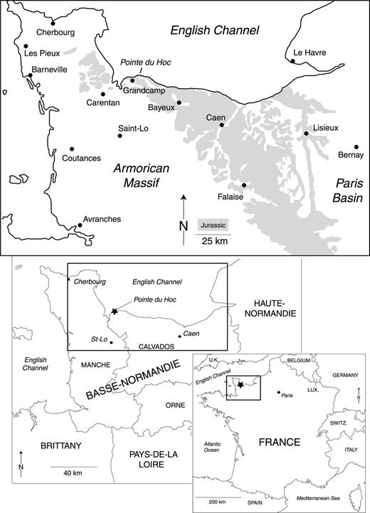
Outline maps showing the location of Pointe du Hoc in Normandy, France. Jurassic outcrops in the region between the Paris Basin and the Armorican Massif are shaded.
Today, the Pointe du Hoc battlefield remains strewn with hundreds of bomb craters and massive chunks of corroding reinforced concrete blasted apart by explosions. Many of the original fortifications however have been left in place at the site. The most important example is the OP building, on top of which the Ranger Monument has been in place since 1979. This building is perched at the most northern position on the promontory and offers a commanding view of the Channel. The OP has been closed to visitors since 2001 due to significant cliff collapses in the vicinity and fears of additional mass movement. Another fortification of great historical significance is the anti-aircraft (RCP) building which is located perilously close to the cliff edge ∼260 m eastwards of the OP building.
Fig. 2 is an aerial view of the site showing the two major at-risk buildings of historical significance. The OP, which constituted the Wehrmacht command centre for the entire Pointe du Hoc battery, is the largest building on site. The main historical significance of the anti-aircraft east (RCP) building derives from its use as the Rangers command post while the invasion unfolded.
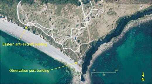
An aerial view of Pointe du Hoc showing locations of the two major at-risk buildings.
2.1 Geological setting
The complex geological history of the English Channel area (Lagarde et al. 2003) has shaped the study area. Tectonic deformation of the middle Jurassic carbonate platform is the likely origin of many of the folds and fractures that are evident in the cliffs today. Tectonic movements associated with Cenozoic uplift and Plio–Pleistocene sea level changes periodically exposed and submerged the coast (Bates et al. 2003; Dugue 2003).
The Quaternary sediment cover throughout the region is typically a quartz-calcareous, homogeneous loess (Antoine et al. 2003). Much of the loess accumulation, typically 2–8 m thick throughout the region, is attributed to the Weichsel glaciation between 15–25 ka. Large quantities of silt reworked from calcareous detrital sediments lying on the exposed floor of the English Channel were blown into the region by prevailing northwest winds.
The Jurassic outcrops at the Pointe du Hoc cliffs are mixed carbonate and siliciclastic rocks that lie between the western margin of the Paris Basin and the eastern margin of the Armorican massif (Fig. 1). The rocks occupy the lower to middle Bathonian (∼165 Ma) stage of the Normandy reference section (Fig. 3) (Rioult et al. 1991). The basal unit of the Pointe du Hoc cliff section, exposed ∼2–3 m above the beach, is the Marnes de Port formation which is a fine clastic alteration of marls and limestones. The overlying bedrock formation is the Calcaire de Creully (also known as Calcaire de St. Pierre du Mont) which is an ∼16-m-thick system of fractured limestones alternating with hard sandstones. The top layer is an ∼8-m-thick layer of unconsolidated Pleistocene silty clay soils. The general stratigraphy at the OP site based on borehole information (Briaud . 2008) is shown in Fig. 4.
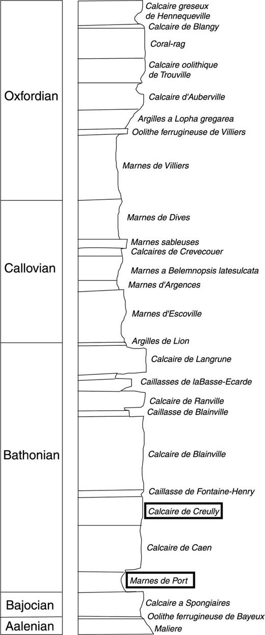
The middle-upper Jurassic succession of the Normandy reference section; outlined are the Bathonian formations found at Pointe du Hoc; after Rioult et al. (1991).
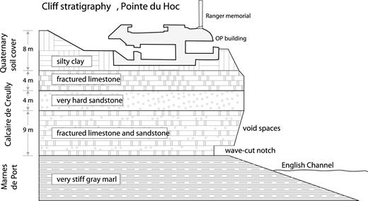
Pointe du Hoc cliff stratigraphy based on borehole information acquired by the Texas A&M geotechnical team. The top of Marnes de Port is roughly the depth of the water table at the site (Briaud et al. 2008).
2.2 Hydrogeology
Assessment of the geological stability of the cliff at Pointe du Hoc requires knowledge of the prevailing hydrogeological conditions. Tidal currents are effective at removing sand from the beach, transporting it >100 km eastwards (Anthony 2002). The beach gravel is washed out to a reservoir ∼100 m offshore during large storms and is redeposited on the beach face during quiet times (Antoine et al. 2003).
The fractures in the Jurassic strata are likely associated with Bathonian and Oxfordian tectonic stresses but many could be of later provenance and/or solution-enlarged by percolating groundwater. There are numerous fractures evident in the cliff face, some of which support vegetation and clearly transmit groundwater. The basal marl unit, in particular, appears to restrict the vertical flow of groundwater as many of the seeps at the cliff face emanate from the top of this layer (Fig. 5). The areas of heaviest vegetation on the Pointe du Hoc cliff face are associated with the groundwater seeps. The seepage is particularly notable during and after the heavy precipitation events. The top of the basal marl (Marnes de Port) layer is also roughly the depth of the water table at the site (Briaud et al. 2008).
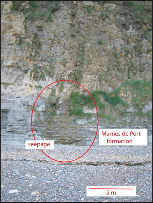
Groundwater seepage from the top of the Marnes de Port formation.
The extensive bomb craters, located in the top soil layers (see Fig. 2), generally do not retain standing water after storms except at the extreme western part of the site where the overlying soil layer thins considerably to less than 1 m. The cliffs are well drained, with infiltrating water readily percolating though the fractures within the limestones and onto the beach. It is likely that groundwater flow through the rock matrix is minimal. Here, as in many other fractured rock systems, the groundwater transport is likely dominated by fissure flow (e.g. Collins 1987; Faybishenko et al. 2005; Neuman 2005).
2.3 Site stability
The existence of historic monuments on the WWII battlefield at Pointe du Hoc is jeopardized by the risk of potentially devastating cliff collapses. These occur frequently along the English Channel coasts of Britain and France. The stability of the Cretaceous chalk cliffs to the east of Pointe du Hoc area has been particularly well studied and a number of important failure mechanisms have been identified (Mortimore & Dupperet 2004). The long-term retreat rate between 1873–2001 of chalk cliffs along the English south coast between Eastbourne and Brighton has been estimated at ∼0.35 m yr−1 based on an analysis of maps and aerial photos (Dornbusch et al. 2008). The cliff retreat rate shows spatial variations that are strongly linked to the local lithology.
There have been a number of large mass movement episodes at Pointe du Hoc in recent history as evidenced by numerous landslide scars near the cliff top, in addition to debris piles and wave-cut notches at the base of the cliffs (Fig. 6). Briaud et al. (2008) report that the rate of erosion of the cliffs between 1944–2006 is ∼0.17 m yr−1. This number was confirmed by the work of Savouret (2007) who, after an extensive study of aerial photographs, found that the rate of erosion of the cliffs from 1823–1944 was 0.18 m yr−1, while between 1944 and 2002 it was 0.15 m yr−1 on the west side and 0.21 m yr−1 on the east side.
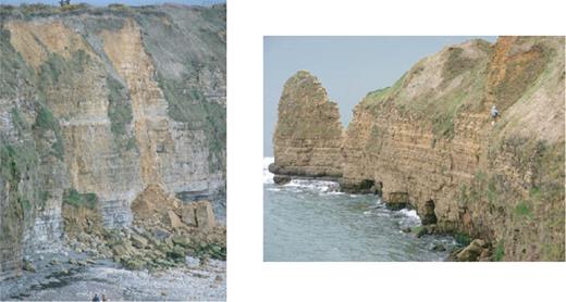
Rock collapses and marine basal notching. (a) A pair of recent collapses on the east side of Pointe du Hoc; note the persons at the top and bottom of the photo for scale; (b) marine basal notching at the bottom of the cliffs; note the rock climber for scale.
Briaud et al. (2008) have suggested failure mechanisms of the cliffs at Pointe du Hoc. Their analysis points to failures occurring via two interconnected processes: (i) slope failure in the top soil cover due to loss of suction after long periods of heavy rains and (ii) overhang collapse in the basal part of the rock cliffs due to sea wave attack.
3 Electrical Resistivity Data Acquisition
Geophysical 3-D ERT data were collected in 2008 February using the ‘SuperSting™ R8/IP’ multi-electrode system manufactured by Advanced Geosciences, Inc. (). This system is widely used for 2-D ERT and 3-D ERT studies. Switching the electrodes to serve as current or voltage pairs is performed automatically according to a sequence that is selected and pre-programmed by the system operator prior to field data acquisition. We used the hybrid dipole–dipole/Schlumberger (DD–Schlumberger) measurement protocol suggested by the manufacturer that combines the good depth of penetration of the Schlumberger array with the superior lateral resolution of the dipole–dipole array. Each resistivity line consists of 42 electrodes with nominal 2.0 m spacing. This permits a maximum n= 39 spacing in the dipole–dipole configuration and maximum AB/2 = 41.0 m in the Schlumberger configuration. The depth of penetration is ∼15–20 m.
On each ERT profile, electrode locations were set out using a tape measure draped across the field topography. Total station surveying was then used to determine 3-D electrode positions to within a few centimetres. The surveying was based on an ad hoc georeferenced control network of ∼20 points that we established at the site. The positions of control points were determined by careful traversing and resection of the network. Overall, this surveying procedure turned out to be a very effective method for precise and accurate navigation of sensor locations in extreme terrain.
The topography of the site required special access to the Pointe du Hoc cliffside. This was facilitated by setting up a safe, releasable rappel system utilizing existing fence posts, historical concrete fragments and, as needed, equalized pickets as anchors. The techniques and technology used in this system are common practice in high angle rescue and recreational climbing. Fig. 6 (right-hand side) shows an example of the cliffside electrode installation that required roped access. Our procedure was as follows: The electrodes were carried down by the climber during a first descent; On the ascent, the electrodes were staked into the cliff face, hooked up to the cable and their positions were recorded using the total station; The climber descended a second time once the ERT measurements were completed and, on a final ascent, unhooked and recovered the electrodes.
The cliffside electrodes are extremely valuable since they permit some of the current injection points to be located on a vertical boundary of the solution domain. This situation is rarely achievable in surface-to-surface ERT geophysics. Conventionally, electrodes can be deployed only on the upper surface of a site to be characterized. In such cases, electric current pathways originate and terminate at the top surface and must pass through the uppermost soil layers, which may or may not be of the primary scientific interest. In the Pointe du Hoc ERT experiment, the cliffside injection points create electric current pathways that originate and/or terminate within the layers beneath the Quaternary soil cover. These pathways provide a unique opportunity for direct energization of underlying Mesozoic strata. Borehole ERT studies (e.g. Daily & Owen 1991) also permit electrodes to be placed directly into the subsurface, but their locations are restricted to reside within an expensive and invasive borehole.
For our study, electrodes could be placed at arbitrary locations on the cliff face. Ordinary steel stakes were used and they were easily hammered into place into the Calcaire du Creully formation without the necessity to drill holes. The contact resistances of the cliffside electrodes were not exceptional compared to those of the topside electrodes. The cliffside electrode lines extend vertically from the clifftop to the base of the Calcaire du Creully formation, which, in most cases, lies within 5 m of the base of the cliff. It proved too difficult for the climbers to hammer electrodes into the underlying Marnes du Port formation.
Separate 3-D ERT resistivity surveys were acquired at the OP and RCP sites. The resistivity data were arrayed in a quasi-regular pattern with a nominal ∼3–4 m line spacing. In some respects, however, the data sets must be regarded as pseudo-3-D since there is always an information gap whenever single-azimuth, or approximately single-azimuth, 2-D data are used in 3-D inversion, as demonstrated by Gharibi & Bentley (2005). The measurement duration of each profile was ∼70 min plus a setup time of ∼45 min for each topside line and ∼3–4 hr for each cliffside line. The capability to lay out an arbitrary pattern of electrodes with respect to an unstructured modelling mesh is preferable to conventional approaches which utilize on-grid electrodes. The latter approaches require manual grid adjustment to accommodate an arbitrary electrode arrangement. The code developed by Li & Oldenburg (2000) allows for electrodes to be placed anywhere within a structured mesh of rectangular cells. Spitzer & Chouteau (2003) describe a case-study with 3-D irregular electrode arrangement; the method of Boulanger & Chouteau (2005) is independent of electrode location; and Johnson et al. (2010) present examples of arbitrary electrode arrangements.
The OP survey consists of 37 resistivity lines, enumerated OP–4 to OP–41, of which 32 are topside lines while five are cliffside lines (Fig. 7). The resistivity lines cover the area around, behind and in front of the OP as well as the surrounding cliff faces. Some of the lines, for example, OP–37 and OP–38, are bent around the OP and thus are sensitive to the geological structure directly underneath it. In general, an excellent spatial coverage of the target area has been achieved. Note that cliffside lines OP–40 and OP–41 have certain electrode points in common. The two lines fan out topside from a shared string of electrodes draped over the cliff. The fan geometry, using shared electrodes, was utilized to take best advantage of the time-consuming cliffside electrode deployment.
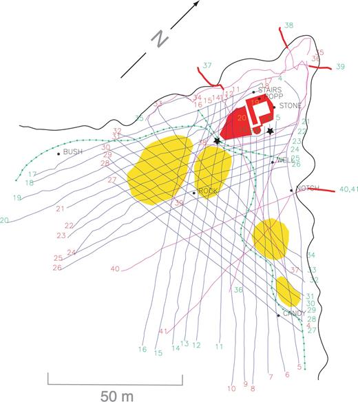
OP geophysical site map showing locations of topside resistivity lines (blue) and cliffside or other lines that required roped access (purple). The start of each line is marked by the green numbers; the end by the red numbers. Green lines are fences; yellow areas are major bomb craters; the OP building is marked in red; the approximate cliff edge is the heavy black line. Names and locations of survey control points are indicated. Vertical parts of the cliffside lines projected onto the horizontal plane are marked with a heavy red line. Borehole locations are marked by stars.
The RCP survey consists of 14 resistivity profiles, enumerated RCP–1 to RCP–14, of which six are topside lines while eight are cliffside lines (Fig. 8). The cliffside resistivity lines also fan out from shared electrode points draped over the cliff. The tomographic coverage at RCP is not as complete as the OP survey since the latter was identified as the highest priority structure; nevertheless a good spatial coverage of the RCP target area has been achieved.
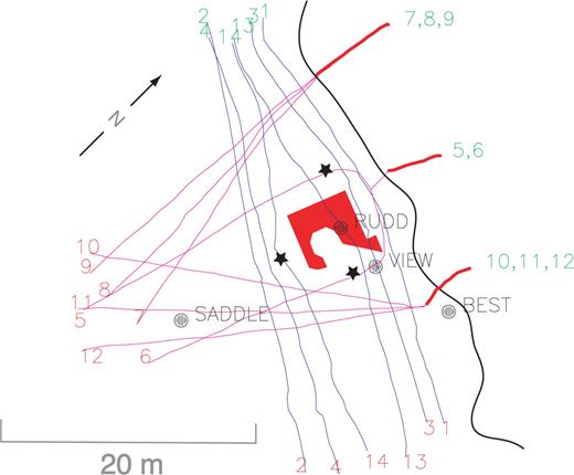
RCP geophysical site map showing locations of topside resistivity lines (blue) and cliffside or other lines that required roped access (purple). The start of each line is marked by the green numbers; the end by the red numbers. The RCP building is marked in red; the approximate cliff edge is the heavy black line. Names and locations of survey control points are indicated. Vertical parts of the cliffside lines projected onto the horizontal plane are marked with a heavy red line. Borehole locations are marked by stars.
4 Data Analysis
The BERT (Boundless Electrical Resistivity Tomography) software package was used to construct the 3-D tomograms; it is based on the inversion method of Günther et al. (2006) and the finite-element forward modelling of Rücker et al. (2006). The software is under active development, open source and available free of charge for academic research (www.resistivity.net). From a variety of data exploration and quality control perspectives, prior to construction of the 3-D tomograms we found it advantageous to conduct preliminary 2-D ERT analyses on individual resistivity profiles.
4.1 Preliminary 2-D data analysis
The initial step of the 2-D analysis is to establish digital terrain files for the individual ERT profiles, using the total station survey data. A terrain file consists, for each electrode, of the elevation and horizontal distance from start of line. The next step is to perform quality control on the measured apparent resistivity data. Poor-quality data points appearing as distinct outliers in the measured pseudo-section are removed. A poor quality datum may be caused by irregular ground coupling of an electrode, faulty connections of cables/electrodes, excessive windy or rainy conditions, extreme near-surface heterogeneities or a low battery. Note that the entire line OP–13 was discarded due to its very poor data quality. It is well known (e.g. Papadopolous et al. 2005; Yang & Lagmanson 2006; Weissling 2008) that 2-D inversions of resistivity data acquired in a demonstrably 3-D environment are problematic to interpret since they contain artefacts due to factors such as geological heterogeneities that reside in whole or in part outside of the vertical measurement plane. Nevertheless, the inverted 2-D resistivity sections at Pointe du Hoc provided us with a rapid and informative overview of the prevailing subsurface conditions prior to the full 3-D analysis.
A few representative 2-D resistivity tomograms from the OP survey area are shown in Fig. 9. These examples illustrate the structural complexity at the site. The top panel corresponds to line OP–5 which, as shown in the survey site map (Fig. 7), runs parallel to the cliff in a southwest direction starting from close to the OP building. The most notable resistivity feature of line OP–5 is the two large, highly resistive (red) zones at >10 m depths. These zones are likely intact, unfractured carbonate-siliciclastic rock blocks. Note that a conductive (blue) zone nests between the inferred bedrock blocks. The high conductivity is likely associated with groundwater accumulation. The line OP–5 also shows small-scale resistivity irregularities at the surface, which are caused either by cultural noise or poor electrode coupling.
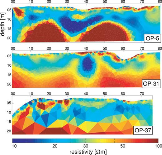
Representative 2-D resistivity tomograms from the OP survey; see text for details. Note that the colour scale is different to the other ERT images shown in this paper.
An interesting elliptical zone of conductive material, above the more resistive bedrock and beneath the near-surface heterogeneity, is evident in line OP–31, as shown in the middle panel of Fig. 9. A similar elliptical zone is also seen at the same location in many of the parallel 2-D resistivity tomograms associated with lines OP–27 to OP–33. The spatial correlation and linearity of the anomaly suggests that this feature might be a hitherto unknown tunnel. The inferred tunnel appears to have disturbed the underlying bedrock, which would have implications for the effort undertaken by the Germans in its original excavation. The high conductivity suggests that the inferred tunnel is either steel reinforced and/or water filled. The dip in the terrain at horizontal location ∼62 m is due to a bomb crater.
A cliffside 2-D resistivity tomogram, line OP–37, is shown in the bottom panel of Fig. 9. There is no vertical exaggeration on these tomograms so that the actual cliffside terrain can be seen along the top edge of the tomogram. This tomogram also reveals the familiar resistive bedrock at depth and the more conductive, less-consolidated materials in the upper layers. Line OP–37 (as shown in the geophysical site map, Fig. 7), passes directly across the concrete apron and staircase on the southern side of the OP building. This explains the large resistive zone in the upper 5–10 m depth range seen at the horizontal locations ∼15–30 m. The three tomograms shown in Fig. 9 are completely different from each other and have different interpretations in terms of buried 3-D features. Overall, the complexity of the 2-D tomograms across the Pointe du Hoc site clearly argues that a 3-D ERT geophysical analysis is needed to avoid misinterpretation of the underlying geoelectric structure.
4.2 3-D terrain analysis
The starting point of the 3-D ERT analysis is to combine all the high-quality 2-D resistivity data into a single 3-D data set that is in the format appropriate for application of the 3-D BERT software. At Pointe du Hoc, the OP and RCP data sets are treated separately. The next step is to establish a fully 3-D digital terrain model of the survey areas. This was achieved by merging the total-station electrode navigation data with terrestrial laser- scanning (e.g. Shan & Toth 2009) data that were acquired at the site.
The laser-scanning measurement campaign, which took place during 2008 February simultaneously with the 3-D ERT geophysical survey, employed a Riegl instrument capable of recording 8000 points of data per second, with 0.01 m distance accuracy at 800 m range. The lidar data set, in the form of an (x, y, z) point cloud, contains not only reflection points on the terrain but also unwanted above-ground reflections from buildings, people, vegetation, fences, vehicles, etc. Using available site photographs, such above-ground reflections were manually identified and removed insofar as possible from the point cloud.
Merging of the total-station and laser-scanning data sets into a single, merged terrain file is straightforward. The electrode positions (xE, yE, zE) are obtained from the total station navigation as described earlier. The horizontal electrode coordinates (xE, yE) are rotated into the same frame of reference used by the laser scanner. This is readily accomplished since there are horizontal control points in common between both data sets. The vertical coordinates zE of the electrodes are then adjusted so that the electrodes are positioned on the terrain, instead of suspended in air or buried inside the Earth. The adjustment is made by raising or lowering the electrode until it matches a local biquadratic function zT(x, y) that is fit using least squares to the digital terrain model derived from the lidar point cloud. In other words, the adjusted vertical coordinate of an electrode in the merged data set satisfies zE=zT(xE, yE).
The 3-D resistivity data sets of the OP and RCP areas, along with the merged digital terrain model, constitute the input to the ‘BERT’ resistivity tomography software package.
4.3 Mesh generation
In extreme terrain, the generation of an appropriate mesh is critical. On one hand, a mesh must be fine enough to capture the spatial variability of resistivity and topography and to ensure an accurate forward calculation. On the other hand, the number of mesh nodes must be limited to keep the run-time low. First, a surface mesh containing the (x, y) positions of the electrodes and given refinement points is generated (Fig. 10a) using constrained triangulation (Shewchuk 2002). This 3-D surface mesh includes an inner region on which the model parameters are defined in addition to an outer region, which is needed for the forward modelling routine. In a second step (see Rücker et al. 2006), an elevation is associated to each node based on the digital terrain file. These nodes are then Delaunay triangulated. Next, the inner and outer regions of the 3-D surface mesh are downwards continued to their desired depths, and region markers are added to the interior and exterior of the modelling domain. The result is then used as input for the tetrahedral mesh generator ‘TetGen’ () whose output is a 3-D volumetric mesh with an inner model-parameter region contained inside a larger forward-modelling region (Günther et al. 2006). A refined mesh is used for the forward calculation, whereas the coarser inner mesh defines the model parameters (Fig. 10b). A similar procedure is performed to create a 3-D volumetric mesh on which to calculate primary potentials (for details see Günther et al. 2006).
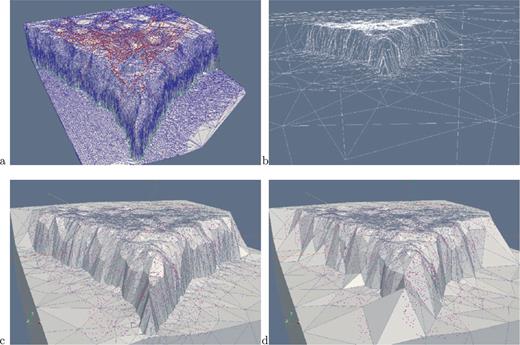
(a) OP Mesh input: topographic points and Delaunay triangulation (blue), electrode positions (red) and supplementary polygon (green); (b) surface mesh with interpolated heights and inner region as input to the ‘TetGen’ mesh generator; (c) final parameter mesh and (d) parameter mesh without the supplementary polygon.
Each surface mesh node has an elevation that is based on linear interpolation of the digital terrain model extracted from the merged lidar/total-station data. However, as the size of the mesh grows towards the boundaries, in rugged terrain some mesh elements near the boundaries may not exactly conform to the topography. For this reason BERT offers the possibility to define supplementary polygons. The polygonal lines are preserved in the surface and volumetric meshes. For example, we included a supplementary line at the base of the cliff where there is a 90° angle to the terrain. Figs 10(c) and (d) shows the surface mesh with and without the supplementary line. The improvement in the definition of the base of the cliff is readily seen. All 3-D figures were produced using the free software ParaView (www.paraview.org).
4.4 Error analysis
The assessment of measurement errors is of critical importance prior to inversion. If a realistic error model is known, data can be fitted within noise, avoiding unrealistically structured or smoothed models by, respectively, overfitting or underfitting the data (LaBrecque et al. 1996).
The data uncertainty δdi is difficult, however, to assess since it is subject to unknown statistical variations. Instrument readings can provide an error estimate based on repeatability. However, this is not a reliable measure as various systematic error sources are not considered. An analysis based on reciprocal measurements (Daily et al. 2004), that is, data that are reacquired after exchanging current and potential electrodes, is preferred. LaBrecque et al. (1996) suggest using an error model based on the observed distribution of residuals δR= (Rf–Rr)/R, where Rf is a forward resistance measurement, Rr is a reversed resistance measurement and R is their average.
Koestel et al. (2008) assume a linear relation δR=a+bR, which is the same as that used by Guenther et al. (2006). Koestel et al. (2008) bin δR according to resistance; then, within each bin the standard deviation is computed. A linear curve is fitted through the standard deviates, yielding the parameters a and b. The number of bins should be chosen such that there is a significant number of data in every bin, but also enough bins to fit a curve appropriately.
The OP data set contains ∼50 000 resistances spanning four orders of magnitude. After deleting bad data we obtained more than 20 000 pairs of normal/reciprocal data. Fig. 11 shows the scatter in the data. The standard deviations within the individual bins are also plotted, together with the fitted error model. We obtained values of a = 1.6 Ω corresponding to 100 μV voltage error and b= 1.1 per cent. The RCP data set yielded values of b= 0.25 per cent and a= 1.4 Ω, or 150 μV.
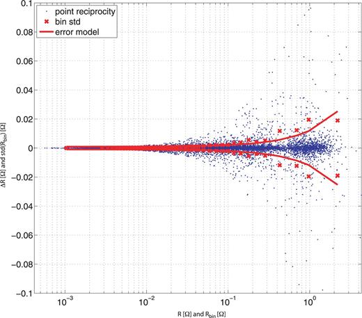
Reciprocity analysis using the OP data set. Measured normal reciprocities (blue) as a function of resistance, bin standard deviation of reciprocity (red crosses) and fitted error model (red line).
While the voltage error seems to be plausible (it is similar to the default value in the BERT algorithm), the percentage error of 1 per cent or less is relatively small. Therefore we have adopted an error floor of 2 per cent to account for error sources that are not exposed by reciprocal measurements.
4.5 Smooth inversion
After mesh generation and error model determination, the next step in ‘BERT’ is to run the full 3-D regularized inversion module, which results in a smooth resistivity tomogram. Some of the parameters used in the 3-D BERT inversions are listed in Table 1. For our study, the Bert package was installed and compiled on a linux system consisting of 16 GB RAM with 8 dual-core processors each working at 2.6 GHz. The number of unknown model parameters approximately equals the number of data. Computing the full Jacobian sensitivity matrix for the OP problem would exceed the available memory and lead to prohibitively long run time. Therefore we used a sparse Jacobian matrix by neglecting values below 10−5. This procedure reduced the storage requirement to ∼5 GB RAM.
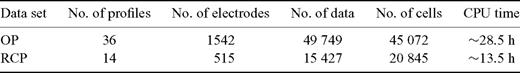
3-D BERT inversion parameters.
The regularization parameter λ controlling the smoothness of the tomogram must be adjusted to generate an earth resistivity model ρ(r) that has a prescribed amount of spatial variability. The choice of λ should also ensure that the data are fitted within their error bounds. Fixing a priori the smoothness of the reconstructed model is a standard, albeit subjective, aspect of geophysical inversion (Constable et al. 1987) and relies on the experience and judgment of the geophysicist. The ‘BERT’ inversion module is run again each time the smoothness parameter λ is adjusted. Generally, there is a wide range of acceptable values of λ for which the structure shown in the tomogram is robust and interpretable from a geological standpoint. For the model parametrization we use a logarithmic transform m = log(ρ−ρL)–log(ρU–ρ) which restricts admissible resistivity values to lie between lower and upper limits ρL= 1 Ωm, ρU= 300 Ωm.
A robust data reweighting scheme (Claerbout & Muir 1973) is used such that data outliers do not have disproportionately large effects on the tomographic reconstruction. Moreover, model responses outside the admissible resistivity range are also downweighted. As a result we find an rms misfit of 21 per cent for the OP data set and 14 per cent for the RCP data set. These rms values are dominated by a limited number of observations with large misfit while the majority of the data are fitted to within a few per cent.
As shown later, the resistivity tomograms show great complexity but this is not very surprising given the site complexity. We tried a number of 3-D inversions using different error models and regularization parameters but they all yielded very similar structures. It is therefore likely that very few of the major features seen in the tomograms are pure artefacts of a non-unique inversion process.
5 Data Interpretation
Interpretation of resistivity tomograms in terms of mass movement hazard at Pointe du Hoc is challenging, especially in view of the strong lithological variations (loess, calcarenite, bioclastic limestone, marl, etc.) and dense cultural clutter that exist at the site. The geophysical data nonetheless provide important information about bulk subsurface resistivity.
The bulk resistivity information contained within a tomographic image is ambiguous relative to an interpretation of the mass movement hazard. For example, a low resistivity zone could be caused by the presence of either clay or groundwater, assuming that the measurements are not greatly affected by the near-surface cultural clutter such as reinforced concrete slabs. Fortunately, the ambiguity is lessened since both clay and groundwater contribute to a weakening of a rock mass as they are both commonly found within fractures and joints. On the other hand, a high resistivity zone in a tomogram could be caused by either an open vug, such as a fracture or a cavern, or a mass of intact rock. The former is associated with weak rock but the latter is characteristic of high strength.
The inherent ambiguities of resistivity tomogram interpretation must be kept in mind when a mass movement hazard assessment is attempted. Incorporation of auxiliary data, such as drill core or geophysical logs, can greatly reduce the inherent uncertainty although these data are typically available at only one or a few discrete points. Several cores of ∼20–25 m length were taken in the vicinity of the OP and RCP buildings by the Texas A&M geotechnical engineering team during drilling at the site in 2006 June and 2008 March. These cores provide important clues as to the nature of the fractures and the geomaterials filling the fractures.
A cursory inspection of a fractured calcarenite core segment from the Calcaire de St. Pierre du Mont formation reveals the presence of two distinct types of fractures. One kind of fracture is open, dry, and contains weathered surfaces. The presence of weathering suggests that water is not being transmitted through this type of fracture. The other type of fracture is wet and filled with a yellowish ochre clay; suggestive of active groundwater processes. These observations suggest that groundwater infiltration and circulation bypass some of the fractures, leaving them open and dry. Much of the groundwater appears to flow preferentially within the subset of wet, clay-filled fractures. The overall strength of the cliff, and its susceptibility to failure, is affected by both types of fracture.
It is known that major wedge failures of the soil at the top of the cliffs occur after periods of heavy rainfall. The infiltration of precipitation and circulation of groundwater adds a dynamic loading to the wet, clay-filled fractures that can trigger their failure. In contrast, the open, dry fractures appear to be passive mechanical elements that respond to the slowly changing, overall stress distribution within the cliff. The stress state of the cliff is largely unknown. The open, dry fractures do not participate in the active groundwater processes and consequently their failure is less predictable, but could occur at any time in the form of a catastrophic topple or rock fall. Nevertheless, for the purposes of this study we assume that the wet, clay-filled fractures are more likely to fail before the open, dry fractures. This is consistent with the general conclusions of Briaud et al. (2008) who emphasize the role of groundwater in the cliff failure mechanisms. Accordingly, a simple conceptual basis for the geohazard interpretation of the resistivity tomograms is introduced in Table 2, in which resistive zones with a moderate mass movement potential are coloured red-orange while conductive zones with a high mass movement potential are coloured blue.
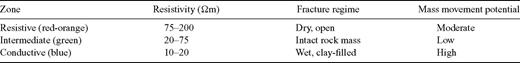
Resistivity tomography interpretation scheme.
5.1 OP data set
Bird's-eye views of the 3-D resistivity tomogram that resulted from the OP geophysical survey are shown in Fig. 12(a) (from a northeast perspective) and Fig. 12(b) (from a northwest perspective). As shown by the logarithmic colour scales, the range of resistivity values extends from log10ρ= 1.0 (ρ= 10 Ωm, shown in blue) to log10ρ= 2.3 (ρ= 200 Ωm, shown in red). The blue colours correspond to relatively conductive Earth materials while the red colours refer to relatively resistive Earth materials. The total resistivity range of the tomogram, from 10–200 Ωm, is modest. The intermediate resistivity value, shown in the green colours, is roughly log10ρ= 1.65 (ρ∼ 45 Ωm) which is intermediate between the bulk resistivity of clay (generally <20 Ωm) and that of limestone (generally >100 Ωm) (Keller 1966).
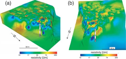
The 3-D resistivity tomogram, based on the OP data set, viewed from (a) the northeast and (b) the northwest. The borehole information is shown: 1 = Quaternary soil cover; 2 = Calcaire de Creully sandstone/limestone; 3 = Marnes de Port stiff marl.
A strong correlation between the borehole-derived stratigraphic information and the resistivity distribution revealed by the 3-D tomogram is not apparent from the external perspective provided in Fig. 12. As shown later, the stratigraphy is revealed more clearly in depth sections cut through the 3-D tomogram. The stratigraphic boundaries are also very apparent in the individual 2-D tomograms shown in Fig. 9.
The main features shown in the OP resistivity tomogram can be identified as follows: First, there are small-scale irregular variations in resistivity scattered across the entire site. These near-surface resistivity variations could be caused either by variations in electrode-ground coupling, variations in soil moisture or by the presence of cultural clutter such as buried reinforced concrete. Most of the surficial anomalies are in yellow to red colours, which indicate that they are due to the resistive near-surface structure. Poor electrode coupling would yield such a resistive signal, as would patches of relatively dry and loose soil. Reinforced concrete can generate either resistive, conductive or complex anomalies depending on several factors, including the moisture content stored in the concrete matrix, and whether the steel reinforcement is in direct electrical contact with the surrounding soil. The signature of the OP building itself is clearly seen in the tomogram. It appears as the prominent circular anomaly consisting of a conductive (blue) inner core surrounded by a resistive (red) halo. The OP has a complicated structure and was constructed by Wehrmacht engineers using ample steel reinforcement.
Another interesting feature of the OP tomogram is the apparent east–west asymmetry of the resistivity structure offshore from the base of the cliffs (see Figs 12a and b). The rocky wave-cut terrace to the west of the point (appearing as a blue-green zone) seems to be more conductive than the gravelly shingle beach to the east of the point (a green-orange zone). This may be an actual effect of subsurface geology, but it should also be mentioned that the west-side resistivity data were acquired predominantly at high tide when the sea was close to the base of the cliffs. The east-side data were taken mainly at lower tide when the sea was further out. The sea is highly conductive, with resistivity ρ= 0.3 Ωm. Thus, the east–west asymmetry shown in the tomogram is likely caused by the proximity of the sea to the electrode profiles at the time of data acquisition.
On both the east and the west cliff faces, there are some interesting resistivity anomalies in the OP tomogram. On the east cliff face, as best shown in Fig. 12(a) there is a distinct resistive zone (shown in orange) located approximately in the middle of the cliff line and continuing down to the beach. This resistive zone indicates a zone of open, dry fractures and, according to the scheme discussed earlier, is assigned as a moderate stability hazard. While the orange zone is certainly an area of concern, a greater risk to the OP is posed by the large conductive anomalies (shown in blue) that lie along the east cliff edge and base in Fig. 12(a). These anomalies are interpreted as zones of wet, clay-filled fractures and are associated with a very high mass movement potential.
On the west face, as shown in Fig. 12(b), there is also a very large resistive (orange) anomaly immediately beneath the OP. This anomaly is interpreted as a zone of a moderate stability hazard. The large conductive (blue) anomaly indicates a greater risk of mass movement hazard as it is interpreted to be a zone of wet, clay-filled fractures. This high-risk anomaly is examined in greater detail in Fig. 13. The OP tomogram is draped over the lidar point cloud and combined with textural information from digital photography. A view of the west-facing cliff is shown. Note that the blue, conductive anomaly is associated with large wave-cut caverns at the base of the cliffs near the promontory. This image indicates that the rocks inside and above the caverns are wet; either from sea water, groundwater or both. The wave action is particularly strong at the position of the blue anomaly because incoming waves from the English Channel are refracted around the headland and their energy is focused on the cliff base at some distance behind the actual promontory.
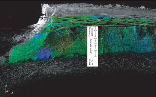
The OP resistivity tomogram draped over the lidar point cloud and combined with textural information from digital photography. The borehole stratigraphic information is shown.
From a geological standpoint, it is not surprising that this region is identified as high risk for mass movement. Consider the geological processes involved in the formation of a sea stack, as illustrated in Fig. 14. Note that the weak area identified in Fig. 14(a) corresponds to the location of the blue conductive anomaly at Pointe du Hoc. In Fig. 14(b), it is seen that, over time, the susceptible area becomes enlarged by erosion to form a sea arch. As shown in Fig. 14(c), further erosion of the arch leads to the collapse of the roof and the formation of an isolated sea stack. This process has already occurred at Pointe du Hoc. In Fig. 14(d), the formation of a series of sea stacks occurs in associated with inland retreat of the headland. This process is occurring today at Pointe du Hoc. The blue conductive zone shown in Fig. 13 (note also there is a second blue zone on the opposite, east-facing cliff close to the promontory) marks a region that eventually will widen and deepen and form a sea arch. When the roof of this sea arch collapses, the OP building may be badly damaged or destroyed.
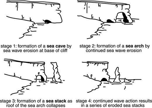
Erosion of a headland resulting in formation of a sea arch and stack; adapted from www.geobytesgcse.blogspot.com.
The formation of a sea stack in a soft coastal cliff environment is a rapid geological process. Historical photographs, for example, reveal that the isolated sea stack now at Pointe du Hoc was connected to the mainland during the 1944 June invasion. Sea arches in general are ephemeral structures that typically survive only a few decades before collapsing, often during great storms.
Due to the great complexities inherent in coastal erosion processes, and the many variables involved, it is not possible to make a definitive prediction of when the putative sea arch at Pointe du Hoc will form and then collapse. Coastal recession is an episodic geological process that is greatly accentuated by events such as large storms, which are inherently unpredictable more than a few days in advance. For evaluation of the erosion risk, coastal engineers largely agree that elements of stochastic modelling and estimation should be included (Hall et al. 2002). Further discussion on quantitative aspects of coastal geomorphology is beyond the scope of this paper.
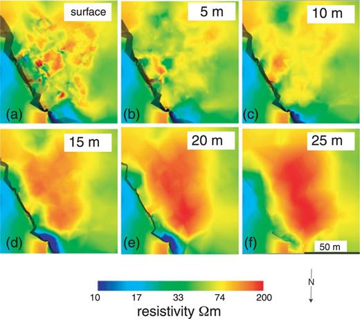
There is much additional information contained in the OP tomogram. The bird’s-eye views shown in Figs 12(a) and (b) reveal only the surface expression of the resistivity distribution. To examine directly the subsurface geoelectric structure it is convenient to take 2-D constant-depth slices through the tomogram. A series of horizontal slices through the OP tomogram at the depths z = 0, 5, 10, 15, 20 and 25 m is shown in Fig. 15. The resistivity distribution within each slice reveals important geological information at the corresponding depth. Note that the topographic datum z of the overall Pointe du Hoc study area is defined relative to the lidar point cloud (Fig. 13), which varies from z=–30 m on the beach to z=+2 m at the southern end of the site. Elevations in the vicinity of the OP building area range, for example, from z∼–5 m at the cliff edge close to the promontory to z∼–2 m at the topmost part of the building.
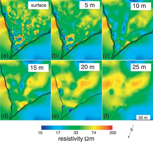
Horizontal slices through the OP resistivity tomogram: (a) surface; (b) 5 m depth; (c) 10 m depth; (d) 15 m depth; (e) 20 m depth and (f) 25 m depth.
An examination of the horizontal slice for depth 5 m (Fig. 15b) reveals that the circular resistivity anomaly associated with the OP building extends at least this far beneath the surface (cf.Fig. 15a). There is a weaker but significant indication of the OP building in the 10 m depth slice (Fig. 15c) but it has essentially disappeared by the 15 m depth slice (Fig. 15d). The lack of a strong OP building signature at depths greater than 5 m suggests that the building foundations are not deeply rooted to the underlying calcarenite/limestone bedrock.
The horizontal slices through the OP tomogram also reveal the presence of a large resistive (orange-red) zone on the west side of the site (the right-hand side of the horizontal slices). The large resistive zone persists to depths >2 m and is accompanied by a second large resistive area below 20 m depth (Figs 15e and f). These resistive zones, according to the scheme in Table 2, are interpreted as areas consisting mainly of open, dry fractures that indicate a moderate mass movement hazard.
In general, the subsurface beneath the OP building becomes more resistive (orange-red) with increasing depth. This trend reflects the fact that the consolidated Mesozoic siliciclastic/carbonate rocks are inherently more resistive than the silty-clay Quaternary cover. Note that, at 10 and 15 m depths (Figs 15c and d), the east side of the site appears in green colours, even though it is composed of Mesozoic rocks. This probably means that the east side is slightly wetter or has slightly greater clay content than the west side, although there is insufficient conductive material on the east side to raise significantly the mass movement hazard potential, which would be indicated in our colour-coding scheme (Table 2) by the presence of a blue zone. In fact, there are few extensive blue regions of conductive materials, interpreted as wet clay-filled fractures, in the vicinity of the OP building. Such blue zones would indicate a high mass movement hazard. There are several small blue areas evident in the 10 m depth slice (Fig. 15c). One that is of particular note, and conceivably caused by a buried cultural structure of unknown provenance, is the linear feature running roughly north–south in the middle of the site landward of the OP building.
A series of 2-D vertical slices through the OP tomogram at 15 m horizontal intervals is shown in Fig. 16. Each vertical slice contains a resistivity distribution that reveals potentially important subsurface information. The prominent linear conductive (blue) zone passing through several of the slices is suggestive of a subsurface cultural feature such as a steel-reinforced tunnel. Further investigation of this intriguing anomaly should be made but it does not appear to be related to cliff stability. Of more concern are the blue zones at the cliff edges. These are indicative of wet clays in the Quaternary soil cover and indicate a high soil wedge-failure hazard. The dry resistive (orange-red) zones along the cliff edges correspond to lower wedge-failure potential.
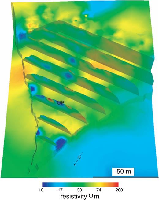
Vertical slices through the OP tomogram. The slices are at 15 m horizontal intervals and extend to 20 m depth.
5.2 RCP data set
A bird's-eye perspective of the 3-D RCP tomogram is shown in Fig. 17. The range of resistivities is similar to that of the OP tomogram. The RCP tomogram shows small-scale irregular variations in resistivity scattered across the topside surface. The signature of the RCP building itself is clearly seen as the prominent quasi-circular anomaly near the centre of the tomogram. The offshore structure appears as a mainly blue region, indicative of the conducting sea water.
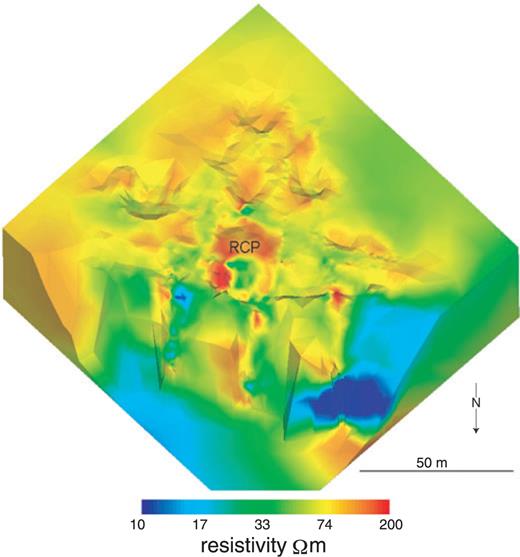
The 3-D resistivity tomogram based on the RCP data set.
There is a very large conductive anomaly (blue) in the RCP tomogram that cuts across the north-facing cliff face to the west of the RCP building. This anomaly is interpreted as a zone of wet, clay-filled fractures. There is smaller blue zone (less prominent; lighter blue colours) on the cliff face to the east side of the RCP building. In general, the cliff face at the RCP site is moderately conductive and represents an area of moderate-to-high mass movement potential. Fig. 6 (left-hand side) shows a pair of recent collapses along the top of the cliff between the OP and RCP buildings. The region around the RCP building might well be the next site of a similar cliff collapse. The next collapse could have potentially damaging consequences for the RCP building.
A series of vertical slices through the RCP tomogram at 15 m horizontal intervals is shown Fig. 18. A series of horizontal slices through the RCP tomogram at the depths z = 0, 5, 10, 15, 20 and 25 m is shown in Fig. 19. Note that the datum z= 0 of the RCP area is based on the lidar point cloud elevation data, which varies from +1.6 m on the top side to –30 m on the beach. The elevation of the cliff edge closest to the RCP building is, on average, –3 m. Both horizontal and vertical slice views of the RCP tomogram reveal that the subsurface beneath the RCP building is very resistive at depth, as shown by the large red zone. Any fractures are likely to be open and dry. Overall, the geoelectrical structure corresponds quite closely to the expected resistivity distribution of a two-layer stratigraphy consisting of Quaternary silty clays overlaying consolidated Mesozoic rocks. There does not appear to be significant blue zones associated with wet, clay-filled fractures beneath the interior of the RCP site. The most conductive zones are found near the cliff edge where both the horizontal and vertical slices show green colours even at greater depth.
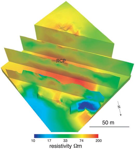
Vertical slices through the RCP tomogram. The slices are at 15 m horizontal intervals and extend to 20 m depth.
Horizontal slices through the OP resistivity tomogram: (a) surface; (b) 5 m depth; (c) 10 m depth; (d) 15 m depth; (e) 20 m depth and (f) 25 m depth.
6 Discussion
The cliff stability assessment at Pointe du Hoc, for the purposes of cultural resources preservation, is a challenging and complex Earth sciences problem that is best addressed using an interdisciplinary approach. A resistivity tomographic solution has been developed, based on rigorous and state-of-the-art geophysical forward modelling and inversion. Within the inherent limitations of the methodology, the subsurface resistivity distribution ρ(r) to the target depths of ∼20–25 m beneath the site has been determined, especially beneath the two major at-risk buildings (OP and RCP) which lie close to the cliff's edge. The resistivity tomography is informed by complementary efforts in terrestrial lidar and geotechnical site characterization.
The lower parts of the resistivity tomograms have been interpreted in terms of sea arch formation and the influence of sea water, yet the data coverage at the base of the cliffs is poor. It would have been desirable to have included horizontal survey lines installed near to the vertical cliff face at beach level. However, this was not done since the semi-diurnal high tide completely inundates the beach. There are only a few hours each day during which beach access is possible.
Geophysics plays a prominent role in the evaluation of cliff stability since electrical resistivity is related to important bulk physical properties such as water content, clay content, lithology and fracture density. These quantities are important factors that control the bulk strength of rock formations and hence the mass movement potential. The complex stratigraphy at Pointe du Hoc, including the clay-silt soils, calcarenites, hard sandstones, bioclastic limestones and marls, in addition to the extreme topography and dense cultural clutter, render electrical geophysics and the interpretation of resistivity tomograms very challenging.
7 Conclusions
3-D resistivity tomography data at Pointe du Hoc have been successfully acquired in the presence of extreme topography and dense cultural clutter. The cliff stability in the areas around the two major at-risk buildings has been analysed. A hazard assessment scheme has been designed in which regions of high resistivity are interpreted as zones of open, dry fractures with a moderate mass movement potential. Regions of low resistivity are zones of wet, clay-filled fractures with a high mass movement potential.
The results of the OP tomography indicate that the highest mass movement hazard appears to be associated with the marine caverns at the base of the cliff that are positioned at the point of strongest wave attack. These caverns likely occupy the future site of development of a sea arch that will definitely threaten the historic building. There is also a high probability of a soil wedge failure on the east-facing cliff edge close to the OP building. Such a failure could damage or destroy the building. The rest of the topside area shows mainly resistive features that are indicative of open, dry fractures. The possibility of a sudden catastrophic failure along any one of these fractures, due to inherent limitations of resistivity tomography as a monitor of bulk rock strength, cannot be ruled out. The mass movement potential at the second site, the RCP area, is low to moderate. The greatest risk at the RCP area is associated with soil wedge failures at the top of the cliffs.
Among geophysical techniques, the resistivity method is generally regarded as the most favourable for providing subsurface information relevant to cliff or slope stability issues. In this paper we have demonstrated how, under difficult circumstances such as challenging terrain and amidst dense cultural signals, an interpretable, high-resolution subsurface image nevertheless can be obtained. A major requirement of the tomographic construction process is the acquisition of high-resolution terrain data; in this case we used lidar scanning and conventional total station measurements. Advanced unstructured mesh generation routines are needed to ensure accurate tomographic inversion. Outstanding challenges that require further research are methods to calibrate resistivity tomograms against geotechnical core and log data, the development of robust petrophysical relationships between resistivity and rock strength and better techniques to discriminate between geological and cultural signals.
Acknowledgments
The project was sponsored by the American Battle Monuments Commission. Thanks to Richard Burt, Richard Carlson, Chris Everett, Josh Gowan, Jason Kurten and Dax Soule for valuable discussions and assistance with the data acquisition. Oliver Kuras and two anonymous reviewers, along with editor Oliver Ritter provided thoughtful comments, which greatly improved the paper.
References
