


Summary
Pure shear wave data are only very rarely acquired for offshore site investigations and exploration. Here, we present details of a novel, seabed-coupled, shear wave vibrator and field data recorded by a densely populated, multicomponent ocean-bottom cable, to improve shallow soil characterization.
The prototype shear wave vibrator uses vibroseis technology adopted for marine environments through its instalment on top of a suction anchor, assuring seabed coupling in combination with self-weight penetration. The prototype is depth rated to 1500 m water depth, and can be rotated while installed in the seabed. The philosophy is to acquire fully complementary seismic data to conventional P- and P-to-S-converted waves, in particular for 2-D profiling, VSP (vertical seismic profiling) or monitoring purposes, thereby exploiting advantages of shear waves over compressional waves for determining, for example, anisotropy, small-strain shear modulus and excess pore pressures/effective stress. The source was primarily designed for reservoir depths. However, significant energy is emitted as surface waves, which provide detailed geotechnical information through mapping of shear wave velocities in potentially high resolution of the upper soil units. To fully utilize pure shear wave content, a proper analysis of surface waves is paramount, due to the proximity of surface wave propagation speed with shear wave velocities.
The experiment was carried out in the northern North Sea in 364 m water depth. Cable dragging was necessary to obtain close receiver spacing (2.5 m effective spacing), with total line length of 600 m. Frequency–waveform transforms reveal both Scholte and Love waves. Up to six surface wave modes are identified, that is, fundamental mode and several higher surface wave modes. The occurrence of these two different dispersive surface wave types with well-resolved higher modes allows for a unique analysis and inversion scheme for high-resolution mapping of physical properties in the shallow subsurface as well as anisotropy, which is discussed in an accompanying paper. The data presented in this paper are thus a unique (long and densely populated receiver array allows for multimodal Love and Scholte surface waves from the marine environment) but challenging (marine operations) marine data set.
1 Introduction: Shear and Surface Waves
Joint analysis of shear (S) wave and compressional (P) wave data yields improved knowledge of the subsurface (Caldwell 1999; Engelmark 2001; Yilmaz 2001; Stewart et al. 2003). Whereas conventional P-wave data are essential to understand margin architecture and sedimentary processes, several instances exist for which either imaging is poor, or data are inadequate in accurately determining in situ properties. This is due to the fact that P-waves sense both matrix and pore fluids, whereas pore fluids influence S-waves to a lesser degree (Caldwell 1999). S-waves have shorter wavelengths resulting in higher vertical resolution and manage to image through, for example, gas clouds, basalts and salt bodies (Engelmark 2001; Yilmaz 2001). S-wave data are not only important for lithology and fluid prediction/discrimination, fracturing and anisotropy, but also to quantify subsurface conditions and constituents, like excess pore pressure (e.g. shallow water flows), saturation, gas and hydrate (Caldwell 1999; Engelmark 2001; Haacke & Westbrook 2006; Westbrook et al. 2008). As shear wave velocity is directly related to small-strain shear modulus—a fundamental geotechnical parameter more closely linked to shear strength than any other geotechnical parameter—shear wave data are highly relevant for geotechnical site characterizations and geohazard studies (Vanneste et al. 2007).
Extracting shear wave information usually involves non-symmetric P-to-S-wave conversions (converted waves) (Thomsen 1999; Stewart et al. 2002) or analysis of subtle amplitude changes (amplitude versus offset/angle, Castagna & Backus 1993). These methods rely on downgoing P-waves, and may fail to deliver as the wavefield itself may be severely attenuated along the travel paths, thereby not generating high-quality S-wave data. Multilevel shallow gas accumulations above leaking reservoirs are classic examples. This calls for using controlled shear wave devices for marine exploration and monitoring, considering that this implies seabed coupling of both source and receivers. However, only very few marine shear wave sources exist. Recently, a reusable implosive source was suggested to generate shear waves, but the drawback was that this source must be returned to the surface between each firing (Dorman & Sauter 2006). A towed sledge system has also been used to map shear wave velocities, but subsurface depth was limited to only a few metres (Winsborrow et al. 2003). To this end, the Norwegian Geotechnical Institute (NGI)—in collaboration with Statoil—designed and manufactured a controlled, robust, fully operational and versatile prototype shear wave vibrator, aiming at illuminating reservoir levels (Westerdahl et al. 2004).
When an elastic/acoustic source is coupled to the seabed, low-frequency surface waves will be emitted (Yilmaz 2001). Their geometrical dispersion and attenuation contain high-resolution information on the shallow subsurface, in particular shear wave velocity (Socco & Strobbia 2004). In vertically layered media, phase velocity becomes frequency dependent and the governing wave equations have multiple solutions for given frequencies, each solution corresponding to eigenfunctions or various modes of propagation (Aki & Richards 2002). These modes should be taken into account when inverting for shear wave velocity (Socco & Strobbia 2004), as they can extend the depth of investigations and increase resolution of the inverted shear wave profile (Xia et al. 2003; O'Neill 2004).
A particular advantage of a shear wave vibrator in combination with three-component ocean-bottom cables (OBCs) lies in the possibility of recording different surface wave types, for example, Scholte and Love waves. These waves have different particle motion and will be recorded on differently oriented receiver components (Semblat & Pecker 2009). Scholte waves are a combination of P- waves and vertically polarized S-waves (SV). Love waves are horizontally polarized S-waves (SH), guided by and trapped within elastic layers, thereby producing multiple reflections. Surface wave analysis is not a common practice in offshore soil investigations (Socco & Strobbia 2004; Eslick et al. 2008). Sometimes Scholte waves are used, as they are easier generated (Bohlen et al. 2004; Shtivelman 2004; Socco & Strobbia 2004; Park et al. 2005). Love waves, on the other hand, are only rarely used [for one example, see Winsborrow et al. (2003)]. This is partly due to the higher attenuation of S-waves in the top few metres (Nolet & Dorman 1996).
Shear wave surveying at the Gjøa field, an oil/gas/condensate field discovered in 1989 in the Norwegian sector of the northern North Sea, was part of extensive activities to better characterize shallow sediments, in particular with respect to geomechanical properties and geohazards, prior to production (started in autumn 2010). The underlying motivation was to investigate a possible shallow water flow risk for ongoing field development using this novel technique, considering the sensitivity of shear waves to effective stress and thus excess pore pressure, as a preparation for the production phase which started in 2010. Therefore, a detailed surface wave analysis was necessary to model the upper soil layers properly. Objectives of this paper are to introduce NGI's novel shear wave vibrator technology for offshore soil characterization, before using field data in particular with respect to surface wave generation, processing and its potential to characterize the uppermost soil layers in a non-invasive way, as a pilot study. Subsequently, field data illustrating multimodal surface waves of both Scholte and Love type are identified and their dispersion curves determined, for both global and local coverage. A follow-up paper discusses joint inversion of these multimodal surface waves in further detail, using a Monte Carlo as well as linearized laterally constrained inversion scheme (Socco et al. 2011). The high amplitude of surface waves implies that careful assessment of their properties is necessary to apply wavefield separation, before shear wave refractions/reflection data can be properly analysed.
2 Geological Setting
The Gjøa reservoir lies on the eastern flank of the Norwegian Channel, a prominent depression that runs parallel to the entire southern Norwegian coastline (Fig. 1) (Ottesen et al. 2005). Sea level fluctuations, changes in oceanographic patterns and dynamics of ice sheets exerted major influences on rates and patterns of sedimentation and erosion during the last 2.5 Myr. Glaciers repeatedly reached the shelf break during the last 1.1 Myr (Sejrup et al. 2000). The last three periods of shelf-edge glaciations of the Fennoscandian ice sheet occurred during the Weichselian (110–10 ka), with ice-free periods in between. Mega-scale lineations in seabed sediments indicate palaeo-ice-stream activity (Ottesen et al. 2005). The Norwegian Channel comprised a convergence of ice streams draining different parts of the Fennoscandian ice sheet (Ottesen et al. 2005), thus soil conditions within the Norwegian Channel may vary significantly from place to place. The last deglaciation started around 18 ka.

Overview map (source: etopo2v2 bathymetry, National Geophysical Data Center) of the northern North Sea showing the location of the seabed-coupled shear wave source experiment at the Gjøa field, on the eastern flank of the Norwegian Channel, a prominent ice-stream pathway (white arrows) through which large volumes of glacial sediments were fed into the North Sea Fan area (solid white line) (Ottesen et al. 2005; Nygård et al. 2007). The outline of the Holocene Storegga landslide (Bryn et al. 2005) is shown by the bold black line. The thin black line marks the border between the Norwegian and UK sectors in the northern North Sea. Shaded areas within the Norwegian sector represent oil, gas and condensate fields and discoveries (source: Norwegian Petroleum Directorate).
The overall stratigraphy in the Norwegian Channel and its flanks reflects these alternations between glacial and interglacial conditions, and is made up of extensive, relatively uniform deformation till sequences separated by glacial erosional surfaces, which in places are draped with a veneer of glacio-marine to marine sediments (Sejrup et al. 2000). At the site of the shear wave source experiment, the seabed is 364 m deep, generally deepening towards the southwest. Local irregularities in seabed morphology, in the form of pseudo-linear depressions, are interpreted as iceberg ploughmark. From 3-D seismic data, the main geological interfaces are flat reflections. The top soil is soft Holocene clays deposited on predominantly glacial to glacio-marine sediment between 170 and 245 m thick, spanning the Quaternary (Nordland Group). Within the Quaternary succession, a number of distinct reflections separate different opaque to semi-transparent units, presumably corresponding to a variety of till deposits. The lowermost Quaternary unit is well stratified and comprises glacio-marine to marine clayey and sandy layers. The Base Quaternary unconformity forms an anticline structure, probably related to the first major cross-shelf advance of the glaciers. It truncates sediments of Eocene age. The hiatus between top Eocene and Base Quaternary is presumably related to erosion following Tertiary uplift of mainland Scandinavia.
A shallow water flow—a sedimentary formation with abnormally elevated fluid pressure underneath a low-permeability formation—was encountered in an exploration well within Eocene sands underneath the anticline Base Quaternary consisting of low-permeable clays.
3 NGI's Prototype Shear Wave Vibrator and Wavefield Generation
3.1 Design
The prototype shear wave vibrator for seabed applications (Fig. 2) was designed and developed by NGI, in cooperation with key hardware suppliers for hydraulics, valves, servo-control, components and assembly, and partner Statoil (formerly Statoil, Norsk Hydro and StatoilHydro). The objective behind the initiative was essentially to illuminate reservoir depths with pure shear waves for advanced seismic profiling or vertical seismic profiling (VSP). The physical principles are similar to those used for conventional land vibrator sources (vibroseis), considered preferable over other types of sources. A hydraulic cylinder, fixed to the rigid part of the foundation coupled to the seabed soil, moves a seismic mass (3700 kg) back-and-forth with low friction at the base, thereby producing a maximum horizontal dynamic force capacity up to circa 250 kN. Stroke is limited to approximately 50 mm. Dry total weight is about 17 tons. The steel ring- or disc-shaped foundation skirt is operated according to well-proven suction anchor principles for deployment and retrieval, and ensures optimum attachment to the seabed with a repeatable seismic coupling. Upon deployment, coupling is guaranteed by self-weight penetration in the soft seabed followed by pumping entrapped water out of the skirts for suction penetration. For release, water is pumped back into the skirts by excess pressure. The source is modular, with the ability to rotate the vibrator part relative to the skirt foundation. Only limited P-wave energy is generated, with the bulk of the energy going into surface waves and downwards emitting S-waves. Skirts can be adapted, dependent on soil conditions, with typically short skirts for stiff soil and deeper skirts for soft seabed conditions. For the field survey discussed here, skirts were 2.5 m deep with 3.25 m diameter. As a contingency, the expensive force generator and control unit of the vibrator can be disconnected from the fairly inexpensive skirts for recovery, in case the unit gets stuck in the seabed.


From top to bottom (a) picture of NGI's prototype seabed source before deployment at Gjøa; (b) snapshots from a remotely operated vehicle of deployment and suction penetration of the vibrator in the seabed; (c) sketch (not drawn on scale) of the most important components of the shear wave source design, with the force, mass, stroke, suction anchor and wavefield generation and (d) orientation and thus polarization of the shear waves can be changed to any direction after seabed installation, maintaining the repeatable seabed coupling.
The prototype is water depth rated to 1500 m, with most of it pressure compensated. Operation depth can be increased by replacing some electronic parts and using longer umbilicals. The source is further equipped with on-board camera, inclinometers, differential pressure sensor, altimeter and accelerometers to monitor seabed operations, behaviour and signal output. The sensors on the source consist of force and stroke for the hydraulic actuator used in closed-loop digital feedback control, accelerometers on the seismic mass and at the outer frame of the source. Most of the system's components for energy supply and data communication are based on standard remotely operated vehicle (ROV)-type of equipment. Electrical energy is supplied by high-voltage (3000 V) transformers through the umbilical cable to a hydraulic power pack unit (HPU) on the source. A CANBUS data network on the source with fibre optic communication through the umbilical, controls data streams to and from the source. Valves and pumps to handle the deployment and recovery are hydraulically operated and controlled through the onboard CANBUS. Source signatures are monitored and controlled through this network. Customized seismic signatures can be generated by the source over a frequency range between about 2 and 60 Hz including pure tones, sweeps, pulses and random signal. Also an earthquake can be simulated. The sole limitation is the performance envelope, restricted by the stroke, hydraulic flow rate and hydraulic pressure capacity (Fig. 3). Ultimately, and in addition to seismic surveying, the design of the vibrator allows for advanced in situ dynamic soil testing under horizontal loading. The procedure of generating shear waves on the seabed is patented (nr. 310747) by NGI. Typical deployment and recovery of the vibrator on/from the seabed takes 15 min.
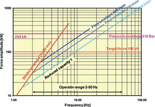
Performance limits of NGI's prototype seabed-coupled wave source: horizontal dynamic force amplitude versus frequency. Performance is limited by three physical constraints, here listed as they are encountered from low towards higher frequency: (red solid lines) maximum possible displacement of sliding inertial body, limited by stroke capacity of hydraulic actuator and of guidance system for inertial body, in combination with mass of inertial body; (blue solid lines) maximum possible velocity of inertial body, limited by flow capacity of hydraulic power supply and of servo valves in combination with piston area of actuator and mass of inertial body. The upper limit is obtained by utilizing hydraulic accumulators. (Purple line) Maximum possible force, limited by maximum hydraulic pressure and piston area of actuator.
3.2 Wavefield generation
The design of the source was complemented with full wavefield simulations to understand and visualize wave patterns emitted by the source, upon horizontal loading of a disc. This is accomplished through 3-D dynamic finite-element (triangular mesh) simulations at single frequencies, accomplished with commercial ‘Comsol MultiPhysics’ code, utilizing perfectly matched layers (PMLs) to enable wave energy to radiate out of the finite-element zone. Simulations illustrate that a complex wavefield is generated by the prototype shear wave source during excitation (Fig. 4). In this visualization, showing total displacement at 16 Hz, the amplitudes from the finite-element simulations are largely exaggerated. In reality, displacements are less than 1 mm, even when the maximum load is applied. The wavefield contains both body and surface waves. Also their spreading pattern or propagation can be detected. Wave types include Love and Scholte waves, S-waves and limited P-waves that will generate reflections and refractions. The small amount of P-waves is caused by tilting movement of the source, causing compression.

Comsol MultiPhysics finite-element simulation of mono-frequency (16 Hz) movement and the wavefields generated from the shear wave vibrator source. The plot shows total displacement. Maximum deformation is approximately 0.4 mm. From this animation (movie available online; see Supporting Information), the different wavefields generated, in particular Love, Scholte and downward propagating S-waves, can be identified.
4 Seismic Data Analysis
Prior to the survey, a careful survey planning was carried out to meet the objectives of the project, which included both surface wave imaging and reflection/refraction shear wave profiling focusing on deeper targets (not further discussed here). The pre-survey planning included design of adequate sweep signatures as well as detailed positioning of the source and receivers, based on high-resolution 3-D seismic and swath bathymetry data (see also Table 1).
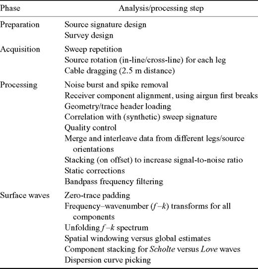
Overview of analysis and processing steps during the different phases of the activities involved.
4.1 Sweep signatures
For this study, the seabed-coupled shear wave vibrator was operated in sweep mode. Prior to the survey, in-depth modelling was undertaken to determine optimal sweep signatures that satisfy two critical conditions: (i) the signature must be strong enough to illuminate target depths for pure shear wave reflections, and (ii) the vibrations generated must not degrade the soil around the skirts. To this end, NGI's in-house geotechnical database was used in combination with our expertise on suction anchor design and dynamically loading foundations. Inertia related to the source's weight and design is taken into account. Two dynamic, horizontal, linear, up-sweep force signatures were provided for the shear wave source to transfer the dynamic force into the seabed at constant amplitude over a fairly wide frequency bandwidth, with exception made for the tapered lead and tail (Fig. 5). The first sweep represents the ideal signal that theoretically should radiate into the subsurface. The second signature is the one imposed on the source, to obtain as close as possible the ideal radiating signature after compensating for inertia from the dead mass of the source and the added interaction soil mass and stiffness. In essence, the designed source signature thus counteracts the loss of amplitudes at higher frequency due to inertia, to obtain a near-perfect sweep signature penetrating the subsurface. The sweep lasted for 7.5 s, and was followed by an equally long listening time. The sweep has frequency content between a few Hertz up to 60 Hz (Fig. 5). Available capacity in stroke, hydraulic flow rate and hydraulic pressure limit force capacity at low frequencies.
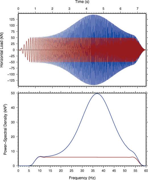
(Top panel) Time-domain representation of horizontal tapered, linear, sweep signatures as programmed for the shear wave source and used for correlation. The signatures are designed to generate enough directional shear wave energy into the subsurface without causing soil degradation of the very soft seabed conditions. The blue sweep signature takes into account frequency-dependent inertia of the source design and surrounding soil in order that—ideally—the red sweep penetrates the subsurface. (Bottom panel) Power-spectral density representation of the sweeps.
4.2 Set-up and field survey
The use of a seabed-coupled shear wave source implies complicated marine operations with two operating vessels and a ROV. The shear wave vibrator source remained stationary throughout the experiment, allowing for rotation in in-line and cross-line directions relative to the receiver array (source polarization). The latter consisted of a 1-km-long, 4-component OBC consisting of 42 accelerometers with 25 m spacing, in split-offset mode (Fig. 6). The cable was deployed partly on the seabed and partly submerged in the water as no lead-in cable was available. To limit spatial aliasing for surface waves, a much smaller spacing between receivers was necessary. This was accomplished by sequentially dragging the cable over 2.5 m intervals, yielding an effective receiver spacing of 2.5 m in the final gathers. At each leg, multiple sweeps were generated, typically six to nine, to allow stacking to enhance signal-to-noise ratio. Sweeps were generated in both in-line and cross-line polarization relative to the cable orientation, to allow both Love- and Scholte-wave types to be generated, in addition to downward emitted SH-waves. In general, source repeatability was reasonable, in particular up to 20 Hz, as indicated by coherency analysis conducted on each pair of data traces for a given leg.
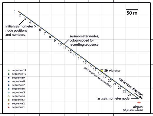
Acquisition layout for shear wave profile at Gjøa. The final multicomponent single-shot gather is made up of 11 cable drag sequences (colour coded), with 2.5 m effective spacing and total length of 600 m. The source positions for shear wave vibrator (yellow square) and airgun (red cross) remained fixed during the survey.
In addition to the shear wave source, a conventional airgun was used to record P wavefield and P-to-SV-converted waves. The airgun was held fixed at the end of the cable at 4 m below sea surface. These data lie beyond the scope of this paper as they are not directly used for analysis or interpretation. However, they were used for properly rotating the OBC components.
4.3 Data processing
Table 1 summarizes the different processing steps undertaken on the data. Isolated noise bursts or spikes were removed by de-spiking. After loading specifications and geometry into the trace headers, seismic traces were correlated with the sweep signature. As several hundreds of sweeps were generated, theoretical sweep signatures that take into account the effect of source inertia (Fig. 5) was used rather than determining sweep-specific signatures using the accelerometers installed on the source as this is a cumbersome and time-consuming task. Comparison with signatures determined from the accelerometers on the source for arbitrary-selected sweeps indicates that there is a reasonable match between the two signals.
The three orthogonal receiver components were rotated into in-line, cross-line and vertical components based on first-break analysis (hodogram analysis) of the airgun records. This is an important step to properly discriminate between the different events within the complicated full waveform data. Shot gathers were subsequently merged and interleaved into an asymmetrical split-spread, 4C 240-channel gather, after which the data were stacked for all shots at the same leg, receiver component and source configuration. This yields a total of six seismic profiles, that is, a triplet of in-line, cross-line and vertical receiver orientations for both in-line and cross-line source polarization. The data were furthermore zero-phase bandpass-frequency filtered (upper frequency 35 Hz) to remove noise trails, likely caused by uncontrolled source vibration or resonance.
5 Results
The time-domain representation of the data is shown in Fig. 7, for the three most important source–receiver combinations, being in-line source orientation with in-line and vertical receiver component, and cross-line source orientation with cross-line receiver component. Surface waves are identified as the steeply dipping (low-velocity), dispersive events. The displays also illustrate the high source repeatability. Other events that are identified are shear wave refractions, its multiples, shear wave reflections and diving waves.
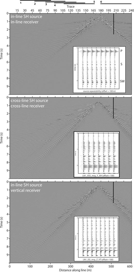
Multicomponent shear wave vibrator data acquired at Gjøa, North Sea. (Top panel) In-line source polarization with in-line receiver registration (Scholte-wave component); (middle panel) cross-line source polarization with cross-line receiver registration (Love-wave component); (bottom panel) in-line source polarization with vertical receiver registration (Scholte-wave components). Surface waves are identified as high-amplitude events with steep dips, thus slow, spreading waves. Other events are refracted or head waves for S, multiple refractions and subtle S-wave reflections. Effective node spacing was 2.5 m, yielding 600 m total line length. Solid lines with indices (1–6) at the top of the figure indicate the locations of the moving windows used in detailed surface wave analysis. The insets illustrate the high source repeatability at given offset.
Vertical and in-line horizontal components contain Scholte wave information, whereas data with the cross-line source with cross-line receiver orientation contain Love wave information.
Due to the dominance of surface wave data on the seismic records, accurate and reliable dispersion curves must be extracted from the field data before proper corrections can be applied to separate different wavefields. Phase velocities of surface waves are only marginally less (say around 10 per cent) than S-wave velocity, which in turn is significantly lower than P-wave velocities in shallow marine sediments, making wavefield separation more challenging using shear wave source data.
5.1 Global surface wave dispersion curves
Several approaches exist to extract dispersion curves from field records (Herrmann 1973; McMechan & Yedlin 1981; Stokoe et al. 1990; Park et al. 1999; Socco & Strobbia 2004; Holschneider et al. 2005; Grandjean & Bitri 2006; Luo et al. 2008). The large number of regularly spaced sensors (240) makes this data set ideal for wavefield transforms, in particular frequency–wavenumber (or f–k) (Nolet & Panza 1976). Data quality is enhanced through zero-trace padding and recovering aliased energy in the negative quadrant. Zero-trace padding (typically 5–10 times the number of available traces) significantly improves wavenumber discretization, whereas phase unwrapping results in doubling the Nyquist wavenumber. The normalized frequency–wavenumber domain representation of the cross-line source orientation with cross-line receiver component, restricted to the longest offset range of the split-spread record, is shown in Fig. 8. Despite the 2.5 m effective receiver spacing, energy is still aliased to some extent (Fig. 8), which would call for even denser population of three-component nodes in the OBC (currently not available). Frequency–wavenumber amplitudes are subsequently mapped into dispersion curves, using the relationship between phase velocity, wavenumber and frequency (Fig. 8).
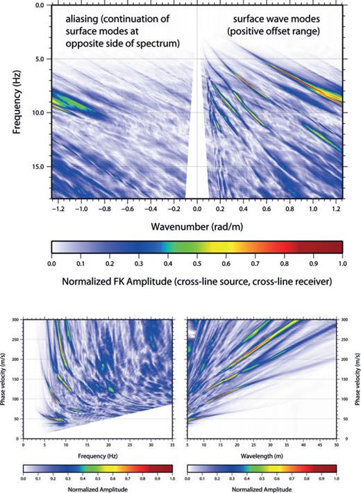
(Top panel) Global f–k spectral image obtained from surface wave data (positive offset range, cross-line source orientation and cross-line receiver, after zero-trace padding) showing multimodal Love waves as high-amplitude events. The spectrum can be unwrapped, by circular shift of negative wavenumbers. (Bottom panel) Global spectra of phase velocities as a function of frequency (left-hand side) or wavelength (right-hand side) from one-sided time-offset data (174 traces), extracted from cross-line source excitation data with cross-line receiver orientation. The high amplitude events correspond to five surface wave modes of Love-wave type. The highest identified mode has lower signal-to-noise ratio.
In case propagated energy also involves higher surface wave modes, different branches of dispersion curve can be retrieved by such spectral analysis. According to the achieved spectral resolution, which mainly depends on the acquisition spread length, the retrieved dispersion curve branches may be related to either fundamental and higher modes or an apparent dispersion curve due to modal superposition. For the global approach focusing on Love waves, five different branches are identified on the spectral images (Fig. 8), which represent the fundamental surface wave mode complemented with four higher surface wave modes. The data clearly illustrate the usefulness of dense geophone spacing in combination with long offset spread which facilitates extracting broad-band dispersion curves, which is important for subsequent inversion (Strobbia 2002; Socco et al. 2011).
The f–k domain data can be analysed either individually or stacked in f–k domain, the latter typically yielding higher signal-to-noise ratios. Spectra with global dispersion curves extracted from the field data are shown in Fig. 8 (Love waves). The picked dispersion curves from the spectral images for individual components are shown in Fig. 9 for both Scholte and Love waves. The dispersion curves obtained after stacking the different components yielding Scholte and Love waves, respectively, are shown in Fig. 10. On the latter, there is evidence of even higher surface wave modes, albeit with lower signal-to-noise ratio.
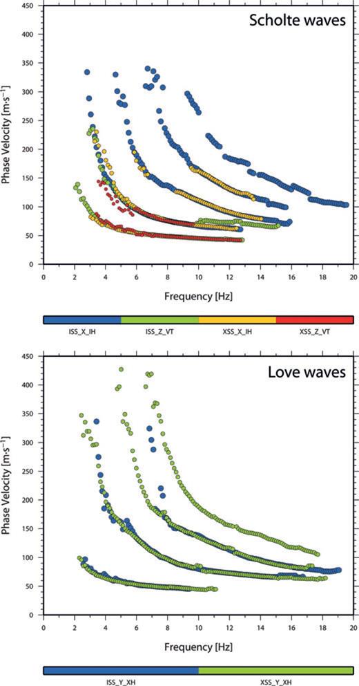
Dispersion curves extracted from field data for different components (X_IH: in-line horizontal; Y_XH: cross-line horizontal; Z_VT: vertical) and source orientations (ISS: in-line; XSS: cross-line) as a global estimate for single-sided offsets for Scholte waves (top panel) and Love waves (bottom panel). These curves correspond to local maxima in the f–k spectra and are interpreted as surface wave modes (fundamental mode and higher order modes) and picked automatically. At least five Scholte modes and four Love modes are distinct on the f–k spectra for all the different components.
Dispersion curves extracted from field data after stacking the spectra for Scholte and Love waves, respectively, resulting in global estimates (320 m window length). The background colour image is the Haskell–Thomson matrix, with the dots representing the picked dispersion curves, that is, the local maxima in the f–k spectra. At least five Scholte modes and four Love modes are distinct throughout the data set on the different components.
At high frequencies, thus representing the uppermost sediments, the phase velocity approaches values less than 50 m s−1. These low values imply that the shear wave velocities in the shallow soil units will be similarly low, indicating very soft clays. At low frequencies, thus for the deeper part of the subsurface, phase velocities reach 350 m s−1 (Scholte) to above 400 m s−1(Love) (Fig. 9). The frequency range of the dispersion curves between 2 and 20 Hz is sufficiently wide to guarantee both high resolution at shallow target depths and reasonable investigation depth. It must be stressed that the maximum investigation depth is determined by the velocities of the materials through which the surface waves propagate. Hence, the low velocities in the shallow soils limit the maximum achievable wavelength. For the slowest branch of the dispersion curve (fundamental mode) with phase velocity around 100 m s−1 at 2 Hz, the investigation depth is predicted to be in the order of 40–50 m.
In case lateral variations in subsurface conditions are anticipated, (tapered) spatial windowing should be considered to extract local dispersion curves. After testing, a relatively wide window of 320 m was used to optimize spectral resolution and improved the bandwidth of the dispersion curve for Monte Carlo inversion purposes (Socco et al. 2011, Fig. 10).
5.2 Local surface wave dispersion curves
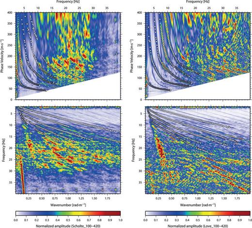
To investigate lateral changes in subsurface shear wave velocities, specific segments were retained from the full profile and processed independently. Six stacked local dispersion curves were retrieved using a 150-m-long moving window with partial overlap (100 m) between neighbouring positions of the moving window (Socco et al. 2011). These windows are indicated on the time-domain seismic data (Fig. 7). Raw data in time-offset domain were tapered with a Hanning window before computing the f–k spectra. Also for local dispersion curves, stacking of Scholte and Love, respectively, was performed. The local dispersion curves also reveal five branches related to different modes of propagation (Fig. 11).

Dispersion curves extracted from field data after stacking the spectra for Scholte and Love waves, respectively, resulting in local estimates using a 150-m-wide window. The background colour image is the Haskell–Thomson matrix, with the dots representing the picked dispersion curves.
6 Discussion: Multimodal Scholte and Love Surface Waves
The two main types of surface waves detected are Scholte and Love waves. Scholte waves have particle motion in the vertical plane of propagation, whereas Love wave particle motion is transverse with respect to propagation direction. As such, Scholte and Love waves are recorded on different receiver components dependent on source polarization (Fig. 9). The pure shear wave, thus Love surface wave, is recorded on cross-line receivers when the source operates in cross-line polarization. Scholte waves on the other hand will occur on in-line and vertical receiver components when the source operates in in-line direction. Ideally, other components would only contain conversions, noise and out-of-plane events.
6.1 Dispersion curves: global and local analysis
The dispersion curves obtained from the stacked spectra (Fig. 10) show five clear and well-separated branches which could be associated to different modes of propagation. Both the curves and the spectra evidence a clear cut-off maximum velocity equal to 350 m s−1 for Scholte waves and around 400 m s−1 for Love waves. These values could be assumed as the value of the velocity in the deepest investigated layer (half-space). Both Scholte- and Love-wave dispersion curves exhibit a low minimum velocity below 50 m s−1 that witnesses the presence of a very soft top layer, that is, the Holocene drape. Similar to even lower surficial shear wave velocities were reported from other geological settings earlier (Winsborrow et al. 2003; Klein et al. 2005; Kugler et al. 2005; Dorman & Sauter 2006). The obtained frequency band (from 2 to about 20 Hz) is wide enough to guarantee both high resolution at shallow depth and reasonable investigation depth. The maximum investigation depth is limited by the low velocity of the materials involved in the propagation that limits the maximum achievable wavelength. Considering the maximum wavelength relative to the slowest branch of dispersion curve, it is reasonable to predict an investigation depth of 40–50 m.
The five local dispersion curves essentially contain information on lateral variations in subsurface conditions. However, the changes are not significant from window to window, indicating that the site itself approaches a flat-layered 1-D medium. Differences in the dispersion characteristics between Scholte and Love waves may provide information on shear wave anisotropy in the shallow subsurface.
7 Conclusions
NGI has successfully designed and operated a versatile seabed-coupled shear wave vibrator to illuminate targets at reservoir depths. To our knowledge, this pilot study in which multicomponent seismic data generated with NGI's prototype shear wave vibrator are recorded, are the first of its kind in the offshore marine environment. The acquisition culminated in an asymmetric, split-spread, three-component, 240-channel shot gather for both in-line and cross-line shear wave polarization, with effective receiver spacing of 2.5 m. Data quality is good.
Inspection of the data indicates that the source emits significant energy as surface waves, in addition to shear wave refractions and reflections. The use of different source polarizations (in-line and cross-line), closely spaced, triaxial receiver nodes and large spatial spreads, allows for detection of both Love and Scholte surface wave types. Frequency–wavenumber spectral images of the recorded data reveal that, for both surface wave types, the fundamental modes as well as several higher modes of excitation occur consistently with high quality. This is to our knowledge the first evidence of jointly recorded, multimodal Scholte and Love surface waves in the marine realm and bears important information on geotechnical properties of shallow soils and anisotropy, a property that is rarely measured.
The dispersions spectrum for the fundamental mode tends asymptotically to 45–50 m s−1 at high frequencies, indicative for shear wave velocity in the uppermost very soft Holocene clays. Such low shear wave velocities explain some spatial aliasing, indicating that—ideally—even denser receiver spacing would be advantageous (around 1 m). The fairly low shear wave velocities encountered imply that the investigation depth sampled by surface waves is limited. This is, however, site specific rather than methodological.
This unique data set allows for an unprecedented joint inversion of multimodal Love and Scholte waves, which may provide high-resolution shear wave profiles over a length of 600 m (see follow-up paper). Joint inversion and the use of multimodal curves have the potential to extend the depth of investigation and shed light on anisotropy at shallow depths.
Despite some uncertainties and irregularities that are not yet fully understood, the geophysical data acquired at Gjøa with NGI's prototype marine shear wave vibrator is a unique and challenging seismic data set. In addition, the field work using the shear wave source would benefit from a densely populated OBC over the conventional cable systems available.
Acknowledgments
The design, development and field survey received support from NGI, Statoil (formerly Statoil, Norsk Hydro and StatoilHydro) and the Norwegian Research Council (Demo 2000). Part of the survey was covered by the Gjøa license partners (Statoil, GDF Suez E&P Norge, Petoro, RWE Dea Norge and Norske Shell). The authors acknowledge Espen Stensrud, formerly at READ AS, for data pre-processing. D. Tollefsrud, K. Tronstad, E. Lied and S.-B. Hansen (NGI) performed field operations, with J.H. Løvholt (NGI) project manager behind the shear wave concept. We express our gratitude to Statoil AS, Gjøa license partners and NGI for permission to publish the data. RXT provided the OBC. The availability of freeware geoscientific source code, for example, Generic Mapping Tools (GMT) (Wessel & Smith 1998) and Seismic Unix (http://www.cwp.mindes.edu) is greatly appreciated. Analysis and processing codes were partly developed within activities at the International Centre for Geohazards (ICG), hosted at NGI. The results described in this paper are partially supported by the Research Council of Norway through the International Centre for Geohazards (ICG). Their support is gratefully acknowledged. This is ICG publication no. 309. We also express our gratitude to the reviewers and editor.
Supporting Information
Additional Supporting Information may be found in the online version of this article:
Movie clip S1.Comsol MultiPhysics finite-element simulation of mono-frequency (16 Hz) movement and the wavefields generated from the shear wave vibrator source. The plot shows total displacement. Maximum deformation is approximately 0.4 mm. From this animation, the different wavefields generated, in particular Love, Scholte and downward propagating S- waves, can be identified.
Please note: Wiley-Blackwell are not responsible for the content or functionality of any supporting materials supplied by the authors. Any queries (other than missing material) should be directed to the corresponding author for the article.
References
Author notes
Now at: Statoil, Drammensveien 264, Vækerø, Norway.
