A benchmark study for glacial isostatic adjustment codes

Summary

1 Introduction

Numerical simulations of glacial isostatic adjustment (GIA) have an important historical role in global geodynamics since they are a key to constrain the rheological profile of the mantle (Cathles 1975) and help in the interpretation of present-day sea level variations and geodetic observations (King et al. 2010). Although various benchmark studies of mantle convection have been successfully completed since the late 1980s (Busse et al. 1994; Blankenbach et al. 1989; Muhlhaus & Regenauer-Lieb 2005; Zhong et al. 2008), to date no extensive GIA benchmark has been published on an international journal of Geophysics, in spite of two remarkable initiatives in the last two decades. In the mid-1990s, a benchmark project for GIA codes was launched by Georg Kaufmann and Paul Johnston. Some results were collated until 1997, when the flow of contribution from the participants ceased (the initial proposal and some results are still available from the web page http://rses.anu.edu.au/geodynamics/GIA_benchmark/). Since the importance of a GIA benchmark was further stated at the eighth European Workshop on Numerical Modeling of Mantle Convection and Lithospheric Dynamics, held in Hruba Skala (Czech Republic) in 2003, another call for an international collaboration was opened. This new initiative, leaded by Jan M. Hagedoorn, was not limited to GIA only but also included the study of the sea level equation (SLE, Farrell & Clark 1976). While some GIA results are still available from the dedicated web page http://geo.mff.cuni.cz/gia-benchmark/, as far as we know the SLE benchmark has never been initiated. Our aim here is to present some results from a new benchmark initiative at a stage in which a significant number of submission has been reached, addressing all of the main aspects of GIA modelling. To strengthen our collaboration (and to increase the probability of success) these activities have been placed in the framework of the European COST Action ES0701 ‘Improved constraints on models of Glacial Isostatic Adjustment’ (see http://www.cost-es0701.gcparks.com/). Our aims are (i) testing the codes currently in use by the various teams, (ii) establish a sufficiently large set of agreed results, (iii) correct possible systematic errors embedded in the various physical formulations or computer implementations and (iv) facilitate the dissemination of numerical tools for surface loading studies to the community and to early career scientists. Though the benchmark activities described here have been initially limited to members of the Action, they will be open to the whole GIA community through the COST Action ES0701 web pages (see ). The collaboration will continue with an SLE benchmark whose details are now under discussion.

There are several motivations for a benchmark study of GIA codes. First, a number of methods and computer packages are now in use from different groups, which include an increasingly sophisticated description of the physics of GIA. Benchmarking the codes, in this context, is useful to strengthen confidence in the results and to validate the methods. A second motivation is the progressively increasing role played by GIA in the framework of global climate change. Fundamental issues such as future projections of vertical crustal movements and sea level variations on a regional and global scale critically rely upon correct modelling of GIA. Predictions of the geophysical quantities involved in this process often depend on several model assumptions and simplifications, whose impact may be crucial for future projections, and that must be verified within a benchmark programme including a significant number of investigators. This would help to identify the most critical issues from a numerical standpoint, and, possibly to determine upper and lower bounds to the errors intrinsically associated with numerical modelling. Third, improvements in modelling techniques are needed to place tighter constraints on ongoing GIA in regions of current ice mass fluctuation. In particular, a benchmark study may be useful for the interpretation of future geodetic measurements in deglaciated areas and for ongoing satellite missions focused on the study of GIA gravity signatures such as GRACE (Paulson et al. 2007; Tamisiea et al. 2007; Barletta & Bordoni 2009; Riva et al. 2009) and GOCE (Schotman et al. 2009; Vermeersen & Schotman 2009). Last, since no GIA benchmark of this extent has ever been accomplished to date (see discussion earlier), it is our opinion that the community could take advantage of the presentation of a number of agreed results obtained from independent techniques which are the basis for future model development. Since some of the scientists working on this benchmark agree to release their numerical codes (and some are available already, see Table 1), we expect that scientists approaching the topic of GIA for the first time could benefit from this project.

Table 1

Top: participating WG COST Action ES0701 members and external contributors (starred), with notes about the independently developed codes and methods. Bottom: contributions to the benchmark tests so far. (Here abbreviation TX/Y denotes test ‘X’ of Test Class ‘Y’.)

Open in new tabDownload slide

Owing to space limitations, a complete review of the GIA theory is not possible here. In the body of the manuscript a basic (but certainly not exhaustive) outline is given to facilitate the reader. A complete summary of state-of-the-art GIA theory is presented in the recent report of Whitehouse (2009). The viscoelastic normal mode (VNM) method for a spherical Earth, introduced in the seminal work of Peltier (1974) and later refined by Wu & Peltier (1982), Sabadini et al. (1982) and Peltier (1985), is at the basis of several numerical contributions presented in this manuscript. An ancillary presentation of mathematical details for the VNM is given by the booklet of Spada (2003), while for a broad geophysical view of the topic the reader is referred to the treatise of Sabadini & Vermeersen (2004). Possible caveats of the VNM approach, particularly regarding the implementation of compressibility and multilayered models in GIA investigations, have been discussed by James (1991) and Han & Wahr (1995), and later reconciled by Vermeersen et al. (1996a) and Vermeersen & Sabadini (1997). In this study, some GIA results obtained by the VNM method are compared to finite elements (FEs) or spectral-finite element (SFE) computations. The applications of these techniques to GIA are briefly summarized in Sections 3.3 and 3.6, respectively.

An important aspect of GIA concerns the rotational variations of the Earth in response to the melting of the continental ice sheets, which is in fact one of the topics of this benchmark. The problem has been stated by Nakiboglu & Lambeck (1980) and analysed in depth by Sabadini & Peltier (1981), who set the theoretical framework which is used in our polar motion benchmark. Then, it was further developed by Yuen et al. (1982), Wu & Peltier (1984) and Yuen & Sabadini (1985). Since the observed secular drift of the rotation axis is currently small (somewhat less than 1 degree Myr⁻¹, see, e.g. Lambeck 1980; Argus & Gross 2004) linearized Euler equations (Ricard et al. 1993) can be employed on the GIA timescales, as done here (for a review of the True Polar Wander problem, which entails the fully non-linear Liouville equations, the reader is referred to Sabadini & Vermeersen 2004, and references therein). The study of polar motion excited by deglaciation has continued through the 1990s (Spada et al. 1992; Peltier & Jiang 1996; Vermeersen & Sabadini 1996; Vermeersen et al. 1997), accompanied by a number of contributions addressing the more general problem of rotational feedbacks, in which sea level fluctuations are driven by the changing position of the Earth's rotation axis responding to unloading (Han & Wahr 1989; Sabadini et al. 1990; Milne & Mitrovica 1996; Sabadini & Vermeersen 1997; Milne & Mitrovica 1998; Peltier 2001; Mitrovica et al. 2005). A further aspect studied is the harmonic degree one displacement, which describes the geocentre motion. Here, GIA contributes a significant secular trend (Greff-Lefftz 2000; Klemann & Martinec 2009).

The paper is organized as follows: in Section 2 the two Test Classes considered in this study are defined and described and their background theory is presented; they pertain to the spectral (2.1) and to the spatial domain (2.2), respectively; numerical methods employed by the contributors are presented in Section 3; results (Section 4) are presented separately for the spectral (4.1) and the time domain analyses (4.2) and discussed in Section 5.

2 Definition of the Benchmark Cases

This benchmark study is mainly focused on the response of a layered, spherically symmetric earth with Maxwell viscoelastic rheology to surface and tidal loads. This section describes a number of relatively simple benchmark cases which can be classified into two tests suites, referred to as Test Class 1 and Test Class 2, illustrated in Sections 2.1 and 2.2, respectively. Test Class 1 (also referred to as ‘wavenumber domain test’) collects case studies that involve the spectral response of the earth model, focusing on loading and tidal Love numbers and their spectra of characteristic times within a range of harmonic degrees (hence the attribute ‘wavenumber’). Love numbers are provided in the Laplace or in the time domain, depending on the solution method employed. Test Class 1 also includes a study of the polar motion transfer function (PMTF), which is pre-requisite to the solution of the Liouville equations. Regardless of the solution method employed, all the Test Class 1 problems can be solved studying the effects of an impulsive (i.e. delta-like) surface or tidal loading to the external surface of the model. In the case studies of Test Class 2 (‘spatial domain test’), we consider loading problems that demand the computation of the surface deformations, gravity and rotational variations in response to finite-size surface loads.

The complexity of the tests proposed here varied from low to moderate, since from our experience in this field and previous benchmark attempts (see Introduction), we know that an agreement on case studies of high complexity is often difficult to reach for various reasons (these include misunderstandings about the theory, unclear specification of problems and human errors). As a consequence, we have made efforts to establish a set of agreed results that can be extended in the future to include more complex case studies. In this respect, the set of tasks proposed here will serve as a basis for other benchmark efforts such as solving the GIA problem by means of the SLE (e.g. Spada & Stocchi 2006). Since intercomparison of codes and techniques is useful to the community and to future GIA investigations, no restrictions have been placed on the solution methods listed in Table 1. However, investigators working with purely numerical methods (e.g. FEs) are mainly involved in spatial case studies (Test Class 2) rather than in wavenumber domain analyses that tend to be difficult (or time consuming) to implement numerically. For this reason, FE investigators Pg and Bl could not provide VNM results. Similarly, predictions based on special Laplace inversion techniques as those employed by Gsa cannot be employed to retrieve the Love numbers spectra in tests belonging to Class 1. Contributors using the VNM theory are able, in principle, to provide solutions to all case studies presented in the following. However, not all available codes produce the necessary output to fill all the entries of Table 1. Solutions obtained using different and independent methods are of particular importance. Hence, the suite of tests will be continued and the results published in a specifically designed web page also open to GIA scientists not involved in this COST Action.

Table 2 provides a list of conventional symbols used throughout the manuscript and the numerical values of constants of interest to the Test Classes to be used in all numerical implementations. The reference model for all benchmark tests (M3–L70–V01) is described in Table 3. Model M3–L70–V01 is characterized by a spherical geometry, it is incompressible, and accounts for self-gravitation of the solid Earth. Mantle layers and the lithosphere have a Maxwell and a purely elastic rheology, respectively; the core is an inviscid fluid and uniform. The viscosity profile of M3–L70–V01, depicted in Fig. 1 by a thick line, corresponds to that of model ICE-3G (Tushingham & Peltier 1991). A special test has been designed for a multilayered viscosity profile, since the determination of Love numbers for finely stratified models has been the subject of investigation during the last decade (see Vermeersen & Sabadini 1997, and references therein). Thus, the benchmark contributors were invited to provide Love numbers for model VSS96 (Vermeersen et al. 1996a) characterized by 28 mantle layers of variable thickness as shown by a thin line in Fig. 1 (the geometry of VSS96 density and shear modulus profiles is fully described in file ‘VSS96.dat’, available from the benchmark web page). Contributors have been also invited to provide results based on variants of M3–L70–V01 according to the type of numerical implementation preferred (e.g. some modellers interested in local investigations may be more oriented to provide flat-Earth computations ignoring self-gravitation at least in a first phase of the benchmark study). Boundary conditions for tidal and loading forcing have been described in a number of previous studies. While there is a consensus about the boundary conditions appropriate for surface loading, core–mantle boundary (CMB) conditions have been the subject of considerable debate in the past (see, e.g. Spada 1995, and references therein). We assume that contributors are using the CMB solid–fluid boundary conditions described by, for example, Wu & Ni (1996), which currently are agreed on within the GIA community.

Table 2

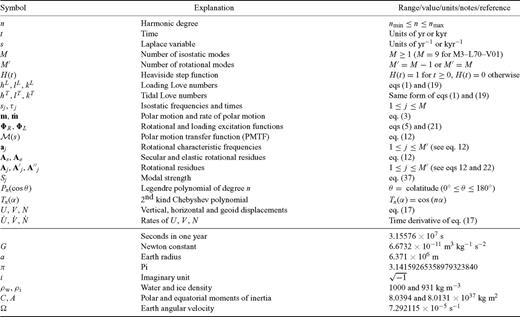
The top part of this frequently used symbols throughout the manuscript. Numerical values of physical constants used as parameters and common to all test suites are shown in the bottom part.

Open in new tabDownload slide

Table 3

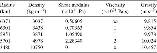
Model parameters for M3-L70-V01, the reference model for this benchmark study. The (unperturbed) gravity at the interfaces is computed according to the reference density profile. These parameters are also adopted in model M3-L70-V01f, the flat-Earth variant of M3-L70-V01 implemented in the FE scheme of Bl (see Section 4.2.3).

Open in new tabDownload slide

Figure 1

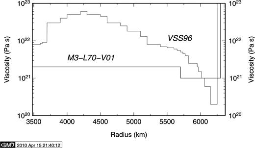
Viscosity profile of models M3–L70–V01 (a three-layer viscosity profile, see Table 3) and VSS96 (a 28-layer profile from Vermeersen et al. 1996a). VSS96 is used in Test 6/1.

Open in new tabDownload slide

2.1 Test Class 1: wavenumber domain

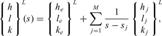
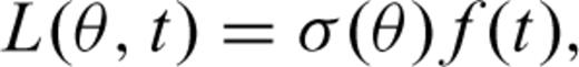
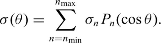
Wavenumber domain tests are designed to provide predictions of loading and tidal Love numbers and to compute the PMTF. Within the VNM method, these quantities computed in the Laplace transform (LT) domain are a pre-requisite for the solution of isostatic and rotational spatial domain problems. For ease of presentation, we only discuss the basic mathematical background, referring to, for example, Spada (2003) for a more in-depth account. The benchmark is presently concentrated on the spheroidal Love numbers and associated field quantities; toroidal Love numbers (Martinec 2007) will be the subject of future investigations.

According to the VNM theory (see, e.g. Spada 2003), the Laplace-transformed loading Love numbers have the spectral form

1

where symbols (h, l, k) refer to vertical displacement, horizontal displacement and incremental gravity potential, L stands for ‘loading’, subscript e denotes the elastic response, s_j are characteristic frequencies, (h_j, l_j, k_j) are the viscoelastic residues associated with each frequency and the dependence on the harmonic degree n is implicit to simplify notation. For the tidal Love numbers (h, l, k)^T(s), which correspond the case of an externally applied potential that does not load the surface of the Earth, a form similar to (1) holds, with the s_j's unchanged since these only depend upon the model structure. For a stably stratified incompressible earth (in which density is constant or increasing with depth), poles s_j are found along the real negative axis of the complex plane, which ensures asymptotically stable time-domain Love numbers. The number M of the viscoelastic modes in eq. (1) scales linearly with the number of layers with distinct viscoelastic properties and is the same for all Love numbers for degrees n≥ 2 (Wu & Ni 1996). In the special case n= 1, the number of modes is smaller than M (Greff-Lefftz & Legros 1997). Since we are dealing with an incompressible model, Love numbers of degree n= 0 vanish.

Elastic Love numbers (h_e, l_e, k_e) are unaffected by the viscosity profile. The same holds true for the fluid loading (or tidal) Love numbers, having both the form

2

obtained by the zero-frequency limit (s↦ 0) of eq. (1).

The VNM method also provides the framework for the description of the rotational response of the Earth to surface loading. In the time domain, the linearized Liouville equations for polar motion read

3

where σ_r is the Chandler wobble (Cw) angular frequency for a rigid earth, is the polar motion vector, ω is the angular velocity vector, Ω is the average angular velocity and

4

is the total polar motion excitation function, which accounts for rotational and a loading deformation through Φ_R(t) and Φ_L(t), respectively (Munk & MacDonald 1975). Eq. (3) is only valid for small displacements of the pole relative to its initial position, an approximation that is appropriate in the context of GIA. The rotational excitation function is

5

where k^T(t) is the tidal Love number of degree n= 2, k_s is the degree 2 secular tidal Love number (Munk & MacDonald 1975) and * is time convolution. Substitution of (4) into (3) using (5) gives the Liouville equations in the form

6

where δ(t) is Dirac's delta. Solving eq. (6) may be tackled in two ways. The first way is simply to neglect the term , which is physically justified considering that the timescale of GIA (a few thousands of years) largely exceeds the Cw period for a rigid earth (∼10 months). In this case, the LT of (6) is

7

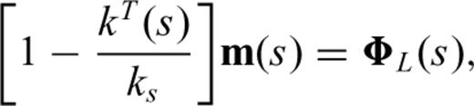
where is the LT of . In the second way, the term is not neglected, which gives the ‘exact’ LT of Liouville equations

8

where the initial condition

9

has been explicitly assumed.

Eqs (7) and (8) can be transformed into a convenient spectral form

10

where is the PMTF. Physically, represents the displacement of the instantaneous pole of rotation for a unit loading excitation in the frequency domain. Assuming

11

the PMTF can be expanded as

12

where the a_j, which are roots of a degree M′ polynomial dispersion equation, represent the (complex) rotational counterparts of the isostatic frequencies s_j in eq. (1). Terms A_e (elastic), A_s (secular) and A_j are (complex) rotational residues. Their amplitude and the value of M′ in eq. (12) depend on the way the Cw is accounted for. In particular

13

whereas

14

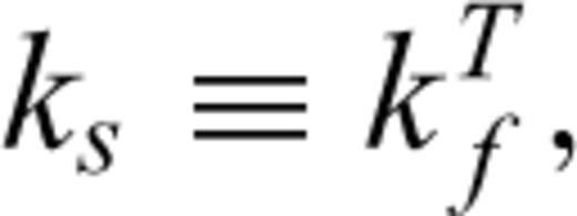
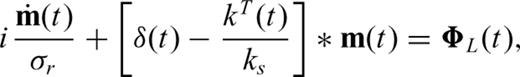
We note that assumption (11) implies that the Earth is rotating in a state of hydrostatic equilibrium before loading. This corresponds to the usual assumption in GIA modelling where any non-hydrostatic effect from mantle convection on the shape of the rotating Earth is normally ignored, as discussed by Mitrovica et al. (2005). Furthermore, since in our GIA modelling we employ a perfectly elastic lithosphere, eq. (11) is not adequate for modelling of long-term polar motion because it implicitly accounts for a finite lithospheric strength. Aware of those issues, we have decided to benchmark results based on eq. (11) because it constitutes the starting point towards more advanced forms of the Liouville equations, in which, for example, k_s≡k^T_obs, where k^T_obs is the currently observed tidal Love number of degree 2 (Mitrovica et al. 2005). However, since eq. (11) has been recently the source of considerable debate (Nakada 2002; Mitrovica et al. 2005; Nakada 2009; Peltier & Luthcke 2009), this issue will be addressed within our ensuing SLE benchmark tests.

2.1.1 Test 1/1. Isostatic relaxation times

This test consists in the computation of the (isostatic) relaxation times τ_j≡−1/s_j(j= 1, … , M) for model M3–L70–V01 (see Table 3) in the range of harmonic degrees 2 ≤n≤ 256.

2.1.2 Test 2/1. Loading Love numbers

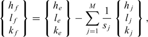
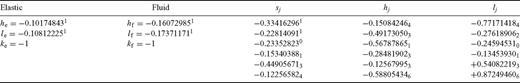
In this test, the computation of the elastic (h_e, l_e, k_e)^L and fluid (h_f, l_f, k_f)^L Love numbers is required (all these quantities are non-dimensional). Residues (h_j, l_j, k_j)^L (j= 1, … , M) are also required. The earth model and range of harmonic degrees are the same as in Test 1/1.

2.1.3 Test 3/1. Tidal Love numbers

This case is the same as Test 2/1, but devoted to the tidal Love numbers.

2.1.4 Test 4/1. PMTF

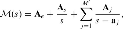
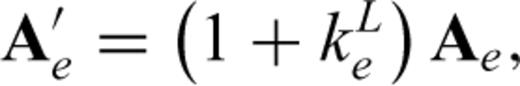
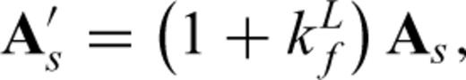
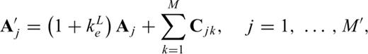
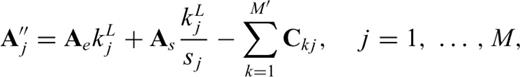
This test applies to the rotational relaxation times a_j(j= 1, … , M′) (kyr⁻¹) and the rotational residues A_e (non-dimensional), A_s and A_j(j= 1, … , M′) (kyr⁻¹), which define the normal mode expansion of the PMTF in the Laplace domain for model M3–L70–V01.

2.1.5 Test 5/1. Time domain Love numbers

This test is suitable for all computation methods that are not based on the VNM theory. For a significant number of degrees in the range 2 ≤n≤ 256, it consists of the computation of the Heaviside Love numbers for model M3–L70–V01 (and possibly its variants) directly in the time domain. The suggested (logarithmically spaced) time window is 10⁻²≤t≤ 10⁶ kyr.

2.1.6 Test 6/1. Love numbers for multistratified models

For the multistratified model VSS96 (28 Maxwell mantle layers, a uniform core, and a homogeneous elastic lithosphere), this test requires the computation of Love numbers in spectral form (by the VNM method) or by any time-domain technique, for a significant number of degrees within the range 2 ≤n≤ 256. The suggested time window is the same as in Test 5/1.

2.1.7 Test 7/1. Love numbers of degree 1

This test requires the computation of the degree n = 1 loading Love numbers, which can be provided in the VNM or in the time domain form. The Love numbers should be expressed in the centre of mass (CM) reference frame (discussion can be found in Greff-Lefftz & Legros 1997), based on model M3–L70–V01 or VSS96.

2.2 Test Class 2: spatial domain

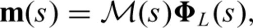
The Class 2 tests concern the computation of surface deformation, geoid height variations and rotational variations (polar motion and length of day) in response to an axisymmetric surface load. If the VNM method is employed, these quantities can be computed starting from the results of the wavenumber tests (see Section 2.1), mainly using convolution methods.

A simple loading episode is simulated employing the loading history f(t) =H(t), where H(t) is the Heaviside function. The load (mass per unit surface) is

15

where θ is the colatitude relative to its axis of symmetry; and the surface mass density σ(θ) is conveniently expanded into a series of Legendre polynomials.

16

The coefficients σ_n can be computed by simple analytical methods (see Spada 2003, and references therein). They are given in Table 4 for three relevant surface loads: the (δ-like) point load, the disc load (with rectangular cross-section) and the cap (parabolic cross-section). Mass conservation is not accounted for in the expressions of σ_n.

Table 4

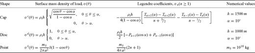
Description of the geometry of the ice loads. For all loads, the ice density is ρ_i= 931 kg m⁻³. The reference value for Earth radius a and the definition of T_n(x), the Chebyshev polynomials of the second kind, are given in Table 2. Here h and α denote the ice thickness and the load half-extension, respectively, while m_δ is the mass of the point load. The Legendre coefficients σ_n are adopted from Spada (2003). Reference numerical values for h, α and m_δ suggested for the spatial domain tests are also given. For Test 2/3, the colatitude and longitude of the centroid of the load geometries are θ_c= 25° and λ_c= 75°.

Open in new tabDownload slide

The response to the load (eq. 15) can be expressed in terms of geodetic variables, which include vertical displacement (U), horizontal displacement (V) and geoid displacement (N) computed at the Earth's surface (r=a). Using standard spectral methods (e.g. Spada 2003), these scalar fields can be cast into the form

17

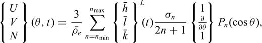
where is the average density of the Earth, and

18

where δ(t) is the Dirac delta function and the n-dependence is implicit. For f(t) = H(t), eq. (18) defines the Heaviside (time domain) loading Love numbers. From the spectral form (1) recalling the basic properties of time convolutions, in this particularly important case we obtain

19

Rates of geodetic quantities at present time (i.e. vertical velocity , horizontal velocity and rate of geoid height variation ), can be obtained computing the time derivative of eq. (17) using eq. (19).

The solution of the Liouville equations in the time domain is obtained starting from the definition of the PMTF (eq. 10). According to Munk & MacDonald (1975), the loading excitation function can be expressed as

20

where ΔI=ΔI_xz+iΔI_yz is the inertia tensor variation due to surface loading. Dynamic compensation is accounted for writing ΔI(t) =ΔI_r(t) * [δ(t) +k^L(t)], where k^L(t) is the loading Love number of degree 2 and ΔI_r(t) is the inertia variation assuming a rigid earth. With ΔI_r(t) =G_σf(t), where constant G_σ is solely determined by the load geometry, the LT of (20) is

21

where f(s) =LT[f(t)]. Substituting eq. (21) into (10) using (12) and recalling the spectral form of Love numbers in the Laplace domain (1), we obtain a further spectral form of polar motion, which now includes loading effects.

22

where the quantity in parentheses only depends on the numerical coefficients that enter the PMTF (eq. 12) and on the loading Love number of degree 2k^L(s). After straightforward algebra one obtains

23

24

25

26

where

27

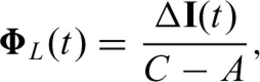
For an Heaviside loading (), the inverse Laplace transform of eq. (22) can be obtained by elementary methods. The result is

28

hence the rate of polar motion is

29

where we note that, consistently with eq. (9), m(0₊) = 0 if the Cw is not neglected in the calculations, whereas m(0₊) = G_σA_e if the Cw is neglected.

A rigorous analytical study of the spectral form of the Liouville equation explicitly yields the condition

30

which, as far as we know, has been first brought to light from Sabadini & Vermeersen (2004) and verified by Vb within the benchmark activities (details available from Vb upon request). Hence, eqs (28) and (29) can be further simplified and expressed in terms of rotational residues A′_s, A′_e, A′_j and characteristic frequencies a_j; isostatic residues A″_j and frequencies s_j do not explicitly contribute to the time domain polar motion.

The geometrical factor G_σ in eqs (28) and (29) can be made explicit following the reasoning of, for example, Spada (2003) that gives

31

where θ_c and λ_c are the colatitude and the longitude of the centroid of the axisymmetric surface load, respectively, and σ₂ is the n= 2 harmonic component of σ(θ) (see Table 4).

Following, for example, Munk & MacDonald (1975), the length-of-day (LOD) variation is

32

where LOD is a reference value of the length-of-day, ΔI_zz is the variation of the axial momentum of inertia in response to loading. Using the expressions given by, for example, Spada (2003) for ΔI_zz, eq. (32) becomes

33

where k^L(t) is the degree two loading Love number for gravity potential. Apart from a scaling factor, ΔLOD/LOD is thus expressed by 1 +k^L(t), a quantity that is benchmarked within Test 5/1. Nevertheless, to facilitate the physical interpretation of the results, LOD computations are explicitly included within Test 3/2 later.

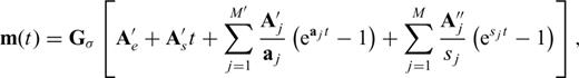
2.2.1 Test 1/2. Geodetic quantities

This test pertains to the evaluation of vertical displacement U(θ, t), horizontal displacement V(θ, t) and geoid displacement N(θ, t). Within the VNM approach, these quantities can be computed using eq. (17) for model M3–L70–V01 (and possibly variants of it) as a function of colatitude θ on a regular angular grid for times t= 0, 1, 2, 5, 10,‘∞’ kyr after the instantaneous loading. For VNM outputs, the range of harmonic degrees is defined by n_min= 2 and n_max= 128. At least one out of the three load models described in Table 4 should be employed. Two grids of different spacing should be used. The first, suitable to visualize near-field results, has the range 0°≤θ≤ 2.5α with a spacing of 0.25°; the second one is global (0°≤θ≤ 180°) with a spacing of 1°.

2.2.2 Test 2/2. Rates of geodetic quantities

This test is identical to test 1/2 above, but ‘rates’ of geodetic quantities [ and ] are to be considered.

2.2.3 Test 3/. Polar motion and LOD

In this test polar motion (eq. 28), rate of polar motion (29) and LOD are considered (33). The surface load, with the same shape and time history as in Tests 1/2 and 2/2, has its centroid at colatitude θ_c= 25° and longitude λ_c= 75°. Values of ..3 and LOD are required at times t= 0, 1, 2, 5, 10,‘∞’ kyr after loading.

3 Methods and Codes

For each contributor, here we briefly illustrate details of the methods and codes employed.

3.1 Gs

Computations from Gs have been carried out using two different methods. The first is the classical VNM method (Gs), implemented within code TABOO, a Fortran post-glacial rebound calculator, while the second (Gsa, see below) is based on a less traditional, recently rediscovered numerical algorithm (code ALMA). TABOO is now part of a more general code (SELEN), which solves the SLE (Spada & Stocchi 2007). The theory behind TABOO is detailed in Spada (2003) and Spada & Stocchi (2006), while the general features of the code are illustrated in Spada et al. (2004). TABOO comes with a user guide, available from http://samizdat.mines.edu. To fit the benchmark requirements, the original structure of TABOO has been modified in a number of points. The most significant modification consists in the implementation of the degree n= 1 loading Love numbers, needed for Test 7/1. In addition, a special script (PMTF, available from the author) has been written with the purpose of computing the numerical coefficients that enter into the PMTF (eq. 12) starting from the degree n= 2 loading and tidal Love numbers obtained from TABOO (Test 4/1). These and other improvements will soon be implemented in a new release of the code (TABOO 2).

3.2 Gsa

Time domain Love numbers provided by ALMA (Gsa) result from the implementation of the Post–Widder Laplace inversion formula (Post 1930; Widder 1934, 1946). The theoretical background is illustrated by Spada & Boschi (2006) while code ALMA is described by Spada (2008). ALMA, which is released under the GNU General Public License (GPL), is now available for download from http://www.fis.uniurb.it/spada/ALMA_minipage.html. In spite of the ill-posedness of the Post–Widder formula (it requires, in principle, the computation of derivatives of order ↦∞ of the Love numbers in the Laplace domain), it has been proven to be especially effective in the case of multilayered models and in the presence of complex transient theologies. For these problems, the root finding algorithms required by the traditional VNM method may fail because of the large number of roots of the secular equation that can be difficult to solve numerically (Spada 2008). Since the Post–Widder formula samples the Laplace transform of Love numbers along the real positive axis (hence the attribute of ‘real’ formula) and no root finding is necessary, in ALMA these problems are overcome preserving, at the same time, the convenient and elegant formalism of the traditional viscoelastic propagators (Spada & Boschi 2006). Major shortcomings of the Post–Widder method, that is, the need of a multiprecision numerical environment and the slow logarithmic convergence to the solution are overcome using public domain packages (Smith 1989) and efficient convergence accelerators (Valko & Abate 2004).

3.3 Pg and Bl

The computations by Pg and Bl were independently performed using the commercial FE package Abaqus (Abaqus 2007). An FE implementation of the GIA equations provides easy access to models with complicated geometry or material parameters varying rapidly in three dimensions or non-linear rheologies (Gasperini et al. 1992; Wu 1992). Wu (1992) described the first implementation of the GIA equations using Abaqus for a flat, incompressible, non-self-gravitating Earth. The Abaqus implementation was later expanded by Wu (2004) to an incompressible spherical, self-gravitating Earth with the SLE included. The Abaqus GIA implementation has been used extensively for studies of lateral heterogeneities (e.g. Kaufmann et al. 1997; Wu & van der Wal 2003; Wang & Wu 2006), non-linear rheology (e.g. Wu 2002a,b), asthenospheric low-viscosity zones (Schotman et al. 2008) optimal placement of new GPS stations (Wu et al. 2010), glacially induced faulting (Lund & Näslund 2009) and, at a smaller scale, current glacial rebound in Iceland (Árnadottir et al. 2009). In the last few years, the FE method has been complemented by the finite volume approach (see e.g. Latychev et al. 2005), which however has not yet seen application within this benchmark.

Commercial FE packages typically solve the Navier–Cauchy equilibrium equations in the absence of body forces, which read

34

where σ is the stress tensor. For an incompressible earth, introducing the body force associated with the gravity field yields to

35

where ρ₀ is density, g₀ is gravity acceleration and w is vertical displacement. Since g₀ is assumed to be constant, eq. (35) does not account for self-gravitation of the solid Earth. To solve it with a commercial FE package (Wu 1992, 2004) it is convenient to redefine the stress tensor to

36

where I is the identity tensor, so that eq. (35) is transformed to ∇·σ′= 0, which is formally identical to eq. (34) hence suitable for the FE analyses. As a result of this transformation of the stress tensor, the stress boundary conditions have to be redefined (for details of this see Wu 2004). These are implemented in Abaqus by supplying Winkler foundations (Williams & Richardson 1991) at all boundaries where the ρ₀ changes, including the free surface. Although strictly defined for an incompressible earth, the Abaqus implementation can be used with compressible materials. However, since gravity is not modelled the compressibility does not produce any buoyancy effect, a condition explored by, for example, Klemann et al. (2003). Bangtsson & Lund (2008) showed that the Abaqus GIA implementation with compressible materials deviates slightly from the correct description, due to the implementation of the GIA terms as surface forces. For a self-gravitating spherical model, the redefined stress tensor has to include also the GIA momentum term relating to self-gravitation. Again, boundary conditions have to be redefined, now also with the gravitational potential. Wu (2004) solves the Laplace equation for the gravitational potential separately, outside of Abaqus, for each iteration of the FE scheme.

In this study, Bl provided benchmark results for the flat Earth Abaqus implementation and Pg independently provided the spherical, self-gravitating Abaqus results. More details on the latter implementation can be found in Dal Forno et al. (2010).

3.4 Rr

The Fortran code FastLove-HiDeg was originally developed by Vermeersen and colleagues (Vermeersen et al. 1996a; Vermeersen & Sabadini 1997) and later improved by Rr to allow the stable computation of high-degree Love numbers (Riva & Vermeersen 2002). FastLove-HiDeg is based on the VNM approach and allows us to compute the response of a spherically layered Maxwell body to different loads. By means of the matrix propagator technique, the problem is solved analytically with the exception of the procedure used to find the roots of the secular determinant (representing the Earth's eigenfrequencies, i.e. the s_j of eq. 1 that is based on a bisection algorithm).

Green's functions are available for both incompressible and compressible rheologies, where the former are directly dependent on powers of the distance from the Earth's centre and the latter are based on the (numerically challenging) spherical Bessel functions. For the incompressible case, the inverse matrices required by the propagator technique are also available in analytical form (Spada et al. 1992; Vermeersen et al. 1996a), while for the compressible case they are computed numerically by Gaussian elimination.

The calculation of the Earth's eigenfrequencies exploits the fact that they change slowly with increasing spherical harmonic degree: after the first set of modes has been determined by finely sampling a broad relaxation spectrum, each individual mode is followed to the next spherical harmonic degree by limiting the search in its immediate neighbourhood, which highly increases the efficiency of the root-finding procedure. To ensure that no important relaxation mode is missing, there is a check on the fluid limit of the Love numbers (see eq. 2), which are also expected to change slowly for increasing degree: when it fails, the root-searching procedure is reinitialized. This last step is particularly important for finely layered earth models, where the frequency of the dominating mode M0 often becomes very close to that of several Maxwell modes. FastLove-HiDeg uses quadruple precision to ensure maximum accuracy.

3.5 Vb

Contributions from Vb have been obtained by an implementation in a symbolic manipulator (Mathematica™4.1) of the algorithm for the analytical evaluation of the Love numbers by means of the matrix propagator technique, within the scheme of VNM theory, whose fundamentals are described by Sabadini et al. (1982), Vermeersen & Sabadini (1997) and Sabadini & Vermeersen (2004). Since the fundamental matrix has elements proportional either to rⁿ or r⁻ⁿ, where r is the radius and n is the harmonic degree (Sabadini et al. 1982), numerical instability arises when the matrix elements exceed machine precision for large n values (see Riva & Vermeersen 2002). To circumvent the problem, all calculations are based on arbitrary-length exact integer numbers of Mathematica™ to secure the highest accuracy until the very end of the calculations, when they are approximated by real numbers or when the roots of the secular determinant and residues are evaluated (Barletta & Sabadini 2006). More precisely, since Mathematica™ can deal with integers (and rational numbers) with an arbitrary number of digits, in MHPLove any real number which is rational is written as a fraction, and irrational numbers such as π have to be approximated by a rational number (by using the Rationalize function). In particular, any input parameter is provided as integer (or rational) number. In this way, since the other internal variables are already in the rational form, any computational operation between numbers gives an exact integer (or rational) result. In detail, after the computation of the determinant of the fundamental matrix as a function of the complex variable s, that is, a polynomial ratio, the numerical evaluation of the polynomial coefficients for s is performed. Then the Mathematica™ root finder is employed (function Solve), and the resulting roots s_j are stored. Each solution s_j is rationalized and used in the fundamental matrix to compute the j-th residue; at this point for the second and last time the numerical evaluation is performed with the n-digit precision (in the contributions presented here n= 100 is used). For this reason, possible ‘numerical’ instabilities (when plotting results) may appear when variables are smaller than 10⁻¹⁰⁰, that is, the effect of the numerical evaluation with the 100-digit precision. Note that, to avoid further numerical inaccuracies, the analytical expression of the residues as a function of s could have been found (leaving the numerical evaluation only after replacing s with the numerical value of s_j), but in this case the CPU (central processing unit) time required by the algebraic manipulator would be exceedingly long.

3.6 Vk

The code VILMA is based on the SFE approach to the forward modelling of the viscoelastic response of a spherical earth with a 3-D viscosity structure loaded by a point mass originally developed by Martinec (2000). For a fixed time, the problem is reformulated in a weak sense and parametrized by tensor surface spherical harmonics in the angular direction, whereas piecewise linear FEs span the radial direction. The solution is obtained with the Galerkin method, which leads to solving a system of linear algebraic equations. Time dependence is treated directly in the time domain as an evolution problem with a homogeneous initial condition prior a surface mass load is applied. The time derivative in the constitutive equation for a Maxwell viscoelastic body is approximated by the explicit Euler time-differencing scheme, which results in time splitting of the stress tensor. Advantages of the method are (i) the explicit time-differencing scheme allows an easy implementation of the non-linear SLE (Hagedoorn 2005); (ii) the extension to lateral variability in viscosity is straightforward and (iii) it allows, in combination with the first aspect, to extend the code to non-linear rheologies (in progress). A previous 1-D version of the code was successfully applied to modelling GIA in several studies (e.g. Fleming et al. 2004; Hagedoorn et al. 2006; Wolf et al. 2006). The influence of rotational deformations on the viscoelastic response was additionally considered in Martinec & Hagedoorn (2005). The code was extended to a 2-D viscosity structure and applied to regional problems (Jacoby et al. 2007; Klemann et al. 2007) and the fully 3-D version is considered in Klemann et al. (2008) and Tanaka et al. (2009) for the problem of postseismic deformation. The compressibility has recently been implemented by employing FEs with a constant density and compressibility (Tanaka et al. 2010). The code is written in FORTRAN; for the 3-D routines, an OPENMP parallelization is applied (OpenMP 2005). For the benchmarks considered in this paper, the 3-D version of the code is used by applying it to the respective 1-D structures.

3.7 Zm

Contributions from Zm have been obtained using code VEENT, which implements the matrix propagator technique in the Laplace transform domain for computing the response of a self-gravitating, incompressible, layered linear viscoelastic sphere to a surface gravitating load. It is based on the analytical formulae for the layer propagator matrix (Martinec & Wolf 1998). Its explicit dependence on the Laplace-transform variable s allows us to determine the amplitudes of viscous (isostatic) modes analytically.

4 Results

4.1 Results for the wavenumber domain

4.1.1 Results for Test 1/1 (isostatic relaxation times)

The spectrum of relaxation times τ_j(j= 1, … , M) for model M3–L70–V01, displayed by small circles, is shown in Fig. 2. The nine branches of the spectrum, labelled according to the usual conventions in VNM theory (Peltier 1985; Spada et al. 1992), include four ‘transient modes’ (T1-T4), a ‘core’ mode (C0), a ‘lithospheric’ mode (L0) and three ‘mantle’ modes (M0, M1 and M2). For insight into the physical origin of these modes and how their number depends upon the complexity of the model, see, for example, Peltier (1985) and Wu & Ni (1996).

Figure 2

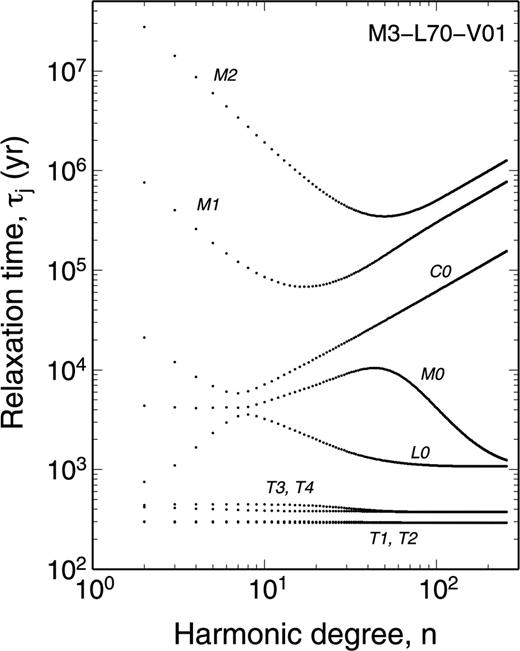
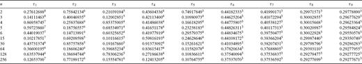
Spectrum of the isostatic relaxation times τ_j, (j= 1, …, M), expressed in years, for model M3–L70–V01 in the range of degrees 2 ≤n≤ 256, according to data sets provided by Vb, Rr, Gs and Zm (Test 1/1). The number of modes is M= 9, branches are labelled according to usual conventions.

Open in new tabDownload slide

In Fig. 2, data from Vb, Rr, Gs and Zm are superimposed and show an excellent mutual agreement with each other. According to Table 5, where numerical values of τ_j are shown for some n values, predictions based on these four independently written codes are in agreement at least in the first six significant figures (this holds for all harmonic degrees in the range of Test 1/1). Considering the distinct approaches followed by the contributors (see Section 3) and by the different numerical implementations, the results of this first test have a particular importance, and confirm that the computation of the isostatic spectrum of incompressible earth models is a straightforward task (Vermeersen et al. 1996b). This is true in spite of some complexity in Fig. 2, as the coalescence of the T modes in the lower part of the spectrum and the crossing of L0, M0 and C0 branches for n≈ 8.

Table 5

Description of the geometry of the ice loads. For all loads, the ice density is ρ_i= 931 kg m⁻³. The reference value for Earth radius a and the definition of T_n(x), the Chebyshev polynomials of the second kind, are given in Table 2. Here h and α denote the ice thickness and the load half-extension, respectively, while m_δ is the mass of the point load. The Legendre coefficients σ_n are adopted from Spada (2003). Reference numerical values for h, α and m_δ suggested for the spatial domain tests are also given. For Test 2/3, the colatitude and longitude of the centroid of the load geometries are θ_c= 25° and λ_c= 75°.

Open in new tabDownload slide

4.1.2 Results for Test 2/1 (loading Love numbers)

Elastic and fluid loading Love numbers, according to Test 2/1, are displayed in Fig. 3, where predictions from Vb, Rr and Gs are superimposed and shown as a function of harmonic degree n. The fluid Love numbers have been computed by all contributors (Vb, Rr and Gs) using eq. (2), which entails the computation of the viscoelastic residues. Alternatively, these could be evaluated via the propagation of the solution through a perfectly fluid mantle up to the elastic lithosphere (Wu & Peltier 1982). This latter approach, which for an incompressible earth merely represents a consistency test, would certainly be extremely helpful in the case of a compressible model, for which the number of normal modes is infinite and their numerical determination is extremely challenging (Vermeersen et al. 1996b).

Figure 3

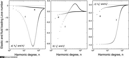
Elastic (e, circles) and fluid (f, squares) loading Love numbers for model M3–L70–V01 as a function of harmonic degree (Test 2/1), computed according to contributors Vb, Rr and Gs. Vertical, horizontal and potential Love numbers are shown in frames (a), (b) and (c), respectively.

Open in new tabDownload slide

The offset between the elastic (labelled by ‘e’) and fluid (‘f’) curves provide, at any given harmonic degree, the total amount of viscoelastic relaxation that each loading Love number undergoes. For small n values, the load is close to a state of perfect isostatic equilibrium in the fluid limit (k^L_f≈−1 in frame c). For sufficiently large n values, elastic and fluid Love numbers reach the same asymptote since loads of sufficiently short lateral extent are fully supported by the elastic lithosphere, which prevents mantle relaxation. All loading Love numbers are negative, with the exception of the horizontal Love number (frame b), which may change its sign in the transition from the elastic to the fluid regime. Interestingly, for degree n≈ 15 the horizontal Love number shows a negligible amount of total relaxation (l^L_e≈l^L_f) but varies substantially between these two states.

From the results of Fig. 3 it is clear that the agreement between predictions of elastic and fluid Love numbers provided by Vb, Rr, Gs and Zm is fully satisfactory. Inspection of some numerical values, displayed in Table 6 for reference, shows that predictions from Vb, Rr and Gs coincide in the first eight digits in the range of harmonic degrees. Small discrepancies are shown for computations by Zm in the case of the horizontal Love number. Although it is not possible to determine which set of Love numbers is ‘correct’ (it is not the purpose of this study), it can be argued that the differences shown in Table 6 reflect differences in the relaxation times (see Table 5). However, it cannot be discounted that they may result from numerical noise in the propagation of the fundamental matrix (see, e.g. Spada 2008), which can affect the computation of the residues and, consequently, the value of fluid Love numbers computed via eq. (2).

Table 6

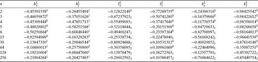
Elastic and fluid loading Love numbers according to predictions from Vb, Rr, and Gs (VRG) for Test 2/1. Results provided by Zm differ from VRG by less than one part in 10⁵ for degrees in the range 2−128. Here y^x and y_x are abbreviations for y× 10^x and y× 10^−x, respectively.

Open in new tabDownload slide

Fig. 4 shows absolute values of residues of the loading Love numbers (i.e. constants h^L_j, l^L_j and k^L_j in eq. 1, respectively), computed by Rr (circles) and Vb (crosses), as a function of degree n in a log–log plot (residues provided by other contributors are not shown for parsimony, but they are available from the benchmark web page). Results from Rr and Vb show smooth, virtually identical branches down to values of ∼10⁻¹⁰ (the same plot would be obtained using data provided by Gs). Since for an incompressible mantle the propagator matrix elements are rational functions of n (see Spada et al. 1990; Wu & Ni 1996; Vermeersen et al. 1996a), oscillating or ‘noisy’ branches should not be observed in the spectrum of residues. A more detailed analysis would show that they may be sometimes visible in the bottom parts of these spectra, for values below ∼10⁻¹³, when the traditional VNM method is employed (Gs and Rr). Since the Vb results remain stable below this threshold, they can be used to test numerical stability of codes. Although these features do not affect significantly the spatial domain results (at least to within one part into 10³), they provide a chance for tuning the numerical methods to improve consistency with other contributors.

Figure 4

Comparison between absolute values of residues of the loading Love numbers computed for model M3–L70–V01 by Rr and Vb (Test 2/1). Smoothness of the nine branches with varying n may indicate that Love number formalism is correctly implemented.

Open in new tabDownload slide

The loading Love number k^L of degree 2 plays a special role, since it defines the loading excitation function for polar motion (see eq. 21). For this reason and to facilitate reproducibility of the results, the spectral components of k^L have been collected in Table 7 (left-hand side), according to contributions obtained from Vb, Rr and Gs. Outputs from these three codes agree to within one part in 10⁸, which is promising for the ensuing polar motion tests.

Table 7

Spectral components of loading Love number k^L (left, Test 2/1) and of tidal Love number k^T (right, 3/1) of harmonic degree n= 2 according to predictions from Vb, Rr, Gs and Zm. All these codes agree to within one part in 10⁸.

Open in new tabDownload slide

4.1.3 Results for Test 3/1 (tidal Love numbers)

Elastic and fluid components of tidal Love numbers h^T, l^T and k^T are shown Fig. 5 as a function of harmonic degree for contributors Vb, Rr and Gs, according to requirements of Test 3/1. As tides only excite the n= 2 harmonic (Munk & MacDonald 1975), the results obtained for n > 2 do not have an immediate geophysical interest. Since computing the tidal Love numbers involves a modification of the surface boundary conditions relative to the loading case (see e.g. Sabadini et al. 1982), the results of Fig. 5 should be regarded as a further validation test of the GIA codes. Love numbers follow smooth curves in the whole range of harmonic degrees, and predictions from the contributors are overlapping. It is worthwhile noting that tidal Love numbers are positive for all n values with the exception of the horizontal ones (frame b), that is, they show a trend opposite to that of loading Love numbers (see Fig. 3). As in the case of loading, elastic and fluid branches of horizontal Love numbers cross each other for n≈ 15.

Figure 5

Elastic (e) and fluid (f) tidal Love numbers for model M3–L70–V01 as a function of harmonic degree n (Test 3/1), computed according to codes Vb, Rr and Gs (results are indistinguishable in this figure). Vertical, horizontal and potential Love numbers are considered in frames (a), (b) and (c), respectively. In frames (b) and (c), low-degree Love numbers are out of range of figure.

Open in new tabDownload slide

To facilitate reproducibility of our results, on the right-hand side of Table 7 numerical values of the spectral components of Love number k^T at harmonic degree n= 2 are shown (results for the whole set of tidal Love numbers are available from the benchmark web page). Similarly to k^L, Love number k^T at degree 2 plays a particularly important role within the theory of the rotation of the Earth, since it defines , the excitation function associated with centrifugal deformation (see eq. 5) and represents one of the basic ingredients of the PMTF . As for the loading case (see Table 7, left-hand side), results from Vb, Rr and Gs agree to within one part into 10⁸.

4.1.4 Results for Test 4/1 (PMTF)

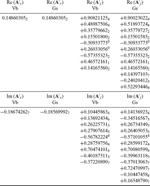
Benchmark results for the PMTF are shown in Table 8, where coefficients A_s, a_j and A_j provided by Vb and Gs are directly compared, with real and imaginary components shown at the top and bottom parts of the table, respectively. The PMTF, which has been computed including the Cw term in the Liouville equations, shows M= 9 and M= 12 modes for Vb and for Gs, respectively (the three extra modes contributed by Gs derive from keeping the three Maxwell modes in the spectrum of isostatic modes). Results pertaining to the case in which the Cw is neglected since the onset of computations, will be employed in the spatial-domain test for polar motion (see Section 4.2.4).

Table 8

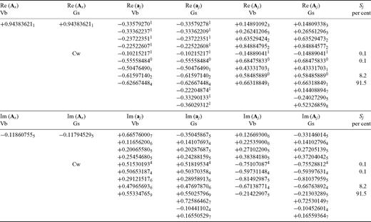
Test 4/1 comparison between real (top) and imaginary parts (bottom) of the coefficients that enter the PMTF contributed by Vb and Gs ( defined by eq. 12). A_s is non-dimensional, all other quantities have units of kyr⁻¹. For both solutions, the Chandler wobble term is included in (the rotational mode carrying the Chandler wobble is marked by Cw). For Gs, M= 12 since the Maxwell modes (of vanishing strength) are included in the Love numbers. Only modal strengths S_i≥ 0.1 per cent are shown.

Open in new tabDownload slide

The agreement between Vb and Gs in Table 8 is good, but some significant differences are clearly seen, especially in the imaginary components of modes with small amplitude (see the first few entries in the lower part of the table). These differences may come as a surprise, given the excellent agreement between Gs and Vb predictions for the isostatic relaxation times and residues (see Sections 4.1.1 and 4.1.2). However, computing the PMTF from these quantities demands, in the Laplace domain, a number of operations with polynomials (including complex root finding) that can cause differences in the final results if not performed with comparable precision of the codes (the algebraic complexity and the pitfalls of the problem is well illustrated by e.g. Wu & Peltier 1984). We have verified that codes employed by Gs and Vb are able to reproduce results based on another three-layer model (Vermeersen & Sabadini 1996), qualitatively showing the same level of misfit demonstrated in Table 8. To appreciate correctly the effective implications of the discrepancies in Table 8, we have computed the strength S_j of the j-th rotational mode, expressed as a percentage in the last column, where strength is defined as

37

Since differences between the stronger modes do not exceed 1 per cent (including the secular term A_s and the Cw term), it is clear that Gs and Vb are effectively producing the same PMTF, in spite of misfits between individual residues evidenced above. The physical equivalence between results from Vb and Gs is confirmed in Section 4.2.4 later, where is employed to compute polar motion in the time domain.

4.1.5 Results for Test 5/1 (time-domain Love numbers)

In Fig. 6 we present results pertaining to loading Love numbers (h, l, k)^L (t) computed in the time domain, in the case of a Heaviside loading, for model M3–L70–V01 (no contributor has provided solutions for tidal Heaviside Love numbers). Three solutions are compared in a time window ranging between 1 and 10⁸ yr, far in excess of the GIA timescales. The first solution (Gs, solid lines, obtained by TABOO) is based on the VNM method. In this case, Heaviside Love numbers are obtained by time-convolution applying eq. (18) in 201 logarithmically spaced points within the time interval considered, with results connected by segments. The second, provided by Vk (open squares), is obtained by an SFE approach using code VILMA, while the third (Gsa, crosses) is based on code ALMA (see Section 3 for details of the codes). For the sake of clarity of presentation, in the case of Gsa the time grid is coarser than the one employed by Vk. Loading Love numbers are computed in three different ranges of harmonic degrees as shown in caption of Fig. 6.

Figure 6

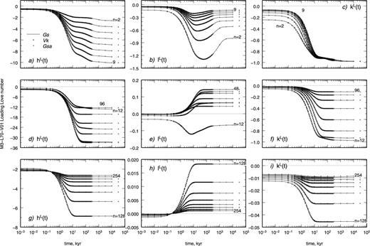
Time-domain loading Love numbers for Test 5/1 in the ranges of harmonic degrees 2 ≤n≤ 9 (top panels), 12 ≤n≤ 96 (middle panels), 128 ≤n≤ 254 (bottom panels). Love numbers have been contributed by Gs (solid lines), Vk (squares) and Gsa (crosses) based on three independent solution methods (see text).

Open in new tabDownload slide

The match between the three solutions in Fig. 6 is remarkable across the whole time window considered. This result is particularly important since these solutions have been obtained with methods (and codes) actually independent one from another. Numerical values of Love numbers, which are provided as accompanying material, will allow the reader to quantitatively appreciate misfits between the results. By visual inspection of Fig. 6, Vk has noted a slight, systematic offset between VILMA and the two competing codes TABOO and ALMA. This can be barely appreciated in frame (i) of Fig. 6, where k^L(t) is computed in the range 128 ≤n≤ 256. Due to the mismatch for large n, Vk, in a second run reduced the step size of the radial FEs in the elastic lithosphere from 5 to 2.5 km. This refinement decreased the deviation from the other two solutions reasonably and confirms the importance of employing semi-analytical tools (e.g. TABOO) to validate numerical codes (and vice versa), especially in the case of computation of short-wavelength (or long-time) limits. The challenging issue of the computation of very large degree Love numbers is not addressed in this study, but would deserve an in-depth analysis due to its relevance in regional investigations of glacio-isostasy (Barletta et al. 2006; Spada et al. 2009). Recently, Spada et al. (2010) have shown that ALMA provides reliable results up to n=O(10⁴), which however are still awaiting for a validation by means of a code based on the VNM method (TABOO fails for very large n values, see Spada 2008) or on FE.

4.1.6 Results for Test 6/1 (Love numbers for multistratified models)

The computation of Love numbers for multistratified models is a challenging problem that has been discussed in length during the past (see, e.g. Vermeersen & Sabadini 1997, and references therein). Using model VSS96, whose viscosity profile is shown in Fig. 1, in Fig. 7 we compare contributions from Vk (SFE method), Gsa (Post–Widder Laplace inversion formula) and Rr (VNM). The complexities shown by VSS96, that is, a low-viscosity sublithospheric region, a relatively large number of layers (28), tiny mantle layers and a low-viscosity core–mantle boundary region, are sufficient to make the computation of Love numbers by the traditional VNM method a difficult task, as illustrated by Spada & Boschi (2006). In particular, as noted by Rr, the complex layering of VSS96 makes it difficult to isolate the fundamental M0 VNM from the relaxation spectrum, where modes are tightly interlaced. For these reasons, Test 6/1 has a particular importance in this study. The direct comparison between contributions from Vk (open squares), Gsa (solid lines) and Rr (dots) in Fig. 7, shows a satisfactory agreement between time domain (Gsa and Vk) and VNM (Rr) Love numbers in the time window 10⁻¹≤t≤ 10³ kyr. Outside this range, Rr and Gsa match very closely. Similarly to the case of M3–L70–V01 (see Fig. 6), discrepancies between Gsa and Vk are visible in the case of Love numbers of large degree (see three bottom frames). Further numerical experiments, whose results are not reported here, have shown that these differences can be mitigated by increasing the spatial resolution of VILMA and/or tuning the number of digits in the multiprecision environment on which ALMA depends.

Figure 7

Time-domain loading Love numbers for Test 6/1 (multistratified model VSS96) in the ranges of harmonic degrees 2 ≤n≤ 9 (top panels), 12 ≤n≤ 96 (middle panels), 128 ≤n≤ 254 (bottom panels). Love numbers have been contributed by Vk (squares), Gsa (solid lines, 201 points in the whole time range) and Rr (dots, 144 points) based on codes VILMA, ALMA and FastLove-HiDeg, respectively. Note that the y-axes range is not the same as in Fig. 6.

Open in new tabDownload slide

4.1.7 Results for Test 7/1 (degree one Love numbers)

Results for degree n= 1 loading Love numbers are shown in Table 9 and Fig. 8. The table shows numerical values of the inverse relaxation times s_j and spectral components of h^L and l^L provided by Vb using the VNM method, expressed in the reference frame with the origin in the centre of mass (CM) of the system (Earth + Load) (see Greff-Lefftz & Legros 1997; Greff-Lefftz 2000). As for the other VNM contributors, the approach to these special Love numbers follows the recipe proposed by Greff-Lefftz & Legros (1997). Note that the k^L Love number is equal to −1; this is true for any possible earth model since this corresponds to the boundary condition of vanishing total incremental potential on the surface of the Earth (Greff-Lefftz & Legros 1997). The elastic solutions are quite close to those pertaining to the homogeneous incompressible sphere (namely h^E=l^E=−1, independently from the physical parameters of the sphere), but the fluid values depart significantly from these values. The VNM solution by Gs and Rr are not reported in Table 9 (but are available from the benchmark web page). Rather, along with solutions by Vb, they are transformed into the time domain by convolution with the Heaviside function, shown Fig. 8 (as far as we know, this is the first time that degree n= 1 Love numbers are shown in this form and benchmarked). The time evolution is complex, but a close agreement between the solutions is apparent. The same holds for Love numbers that are directly computed in the time domain (Gsa, 201 time points in the interval considered) and (Vk, open squares).

Table 9

Spectral form of loading Love numbers of degree n= 1 in the CM provided by Vb for Test 7/1. Others have contributed a different number of modes (M= 9 for Gs and M= 12 for Rr), but the agreement between VNM and time-domain solutions shown in Fig. 8 clearly demonstrates that all the strength is contained in the M= 6 modes reported here.

Open in new tabDownload slide

Figure 8

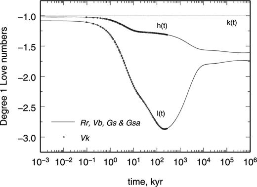
Time-domain loading Love numbers of degree n= 1 for Test 7/1 obtained by contributors Rr, Vb, Gs (by VNM), Gsa (by Post–Widder formula) and Vk (by SFE, squares). Note that k^L(t) = −1 (dashed line).

Open in new tabDownload slide

4.2 Results for the spatial domain

4.2.1 Results for Test 1/2 (geodetic quantities)

In Fig. 9, we directly compare the geodetic quantities U, V and N according to Gs (solid lines, obtained by VNM code TABOO) and Vk (crosses, by the SFE implementation used in VILMA). According to Test 1/2 description, these quantities are shown for different times after loading, as a function of colatitude θ measured with respect to the load centre. For a better visualization of the results, Gs predictions are shown with a spacing of δθ= 0.5° in the range of colatitudes, while for Vk this grid is used only for 0 < θ≤α= 15°; a coarser resolution (δθ= 1°) is employed outside this range. Results for the parabolic and for the disc load are shown in the left and right frames, respectively; in both cases a Heaviside time history is used and mass conservation is not imposed (the load parameters are detailed in Table 4).

Figure 9

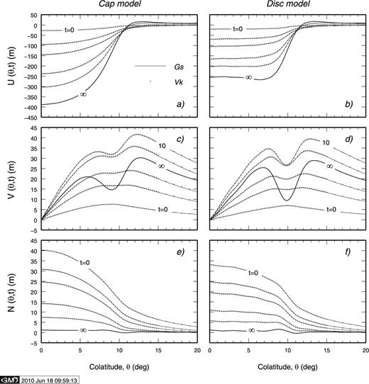
Vertical, horizontal and geoid displacements at the Earth's surface (Test 1/2) according to Gs (VNM method, solid lines) and Vk (SFE, dots) for a cap ice-sheet model (left-hand side) and a disc (right-hand side) imposed at time t= 0. Symbol ‘∞’ stands for t= 10³ kyr for Gs and corresponds to isostatic equilibrium, this datum is not available for Vk.

Open in new tabDownload slide

The results of Fig. 9 pertaining to U (frames a and b) and N (e and d) have an elementary physical interpretation in view of the simple loading time history employed. After the instantaneous elastic response, these fields monotonously evolve to final values in which the load is isostatically compensated. In this state, marked by ‘∞’ in the Gs results (this corresponds to t= 10³ kyr), vertical displacement attains its maximum amplitude, while the geoid undulations are ≈0. Horizontal displacements, shown in frames (c) and (d), vanish for θ= 0° by virtue of the load symmetry and show a more complex pattern with varying θ compared to U and N, with local minima that develop in the proximity of the load margin (θ≈α= 10°). Furthermore, they do not show a monotonous time evolution towards equilibrium; rather, maximum amplitudes are reached at time t≃ 10 kyr, and they decay by a factor of ∼2 before a full compensation is reached. In the range of colatitudes considered, all horizontal displacements are positive (i.e. along the direction of increasing θ, away from the load centre); for large θ values, they change sign (see Table 11).

Table 11

As in Table 10, but for horizontal displacement V(θ, t) in Test 1/2.

Open in new tabDownload slide

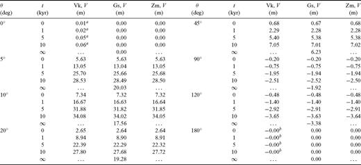
The overall agreement between Gs and Vk is qualitatively apparent from the results of Fig. 9. To provide the reader with a more precise comparison that may be useful for benchmarking their codes, in Tables 10, 11 and 12 we report, in the case of the cap, numerical values of U, V and N for some points of the spatio-temporal grid, also including colatitudes outside the near-field range of Fig. 9 (full arrays of values available from the benchmark web page). The tables compare three solutions, where those of Vk and Zm apply the SFE method and Gs applies the VNM method. In most of the cases presented, differences between predictions are of the order of a few decimetres at most. However at the load margin (θ=α= 10°), discrepancies between Vk and the other two solutions are significantly larger (for vertical displacements, these amount to 1–2 m for times t≥ 1 kyr). The principle difference between the two methods is the handling of the load spectrum. Whereas Gs took the analytical representation of Table 4, Vk and Zm transformed the given shapes numerically into the spectral domain. The results of Zm, which coincides much better with those of Gs, were achieved with a very fine spatial discretization of the load (16 n_max gridpoints) to determine the load spectrum, whereas Vk considered only a grid of 4 n_max points. Vk could show in a further run applying the analytical representation of the spectral load that the discrepancies vanish.

Table 10

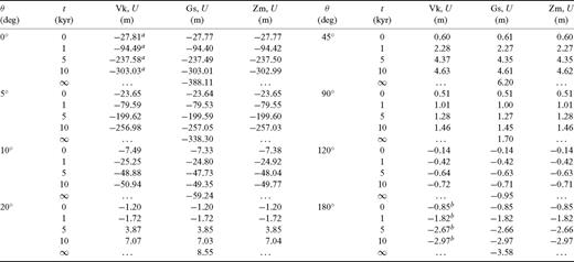
Comparison between vertical displacements U(θ, t) independently computed by Vk, Gs and Zm for Test 1/2 (cap load model). Numbers in parentheses following the contributor abbreviation is time in units of kyr. Units for U, V and N are metres throughout. The figures are obtained by truncating the outputs of codes at the centimetre level. Superscripts a and b indicate that the corresponding quantities are computed by Vk at θ= 0.01° and θ= 179.99°, respectively. Symbol ‘∞’ stands for t= 10³ kyr for Gs. The corresponding values are not available for Vk and Zm, since the computations would require an exceedingly long CPU time.

Open in new tabDownload slide

Table 12

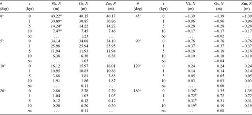
As in Table 10, but for the variation of geoid height N(θ, t) in Test 1/2.

Open in new tabDownload slide

4.2.2 Results for Test 2/2 (rates of geodetic quantities)

Fig. 10 shows the time derivatives of geodetic quantities (Test 2/2), independently computed by Gs (solid lines, VNM) and Vk (dots, SFE) using model M03-L70-V01. Quantities and are computed at times t = 0, 1, 2, 5, 10, ∞ (i.e. 10³) kyr after loading (units are mm yr⁻¹), using the same settings and ice models as in Section 4.2.1. The rates attain their largest amplitude immediately after loading (t= 0) because of the large isostatic disequilibrium and subsequently decrease until the load is fully compensated for sufficiently large times. In the near-field region considered (0°≤θ≤ 20°), vertical displacement is clearly the dominating signal; as a rule of thumb exceed and (which have a comparable magnitude) by a factor of ∼ 10. The agreement between Gs and Vk is satisfactory in all the frames; inspection of numerical values reveals that the misfit between VNM and SFE results are of the order of 0.1 mm yr⁻¹ at most (this misfit level can possibly be reduced acting on the grid spacing in the SFE approach in Vk or refining in the VNM algorithm in Gs). The level of disagreement between the results of Gs and Vk shown in Fig. 10 appears to be significantly smaller than the error bars commonly characterizing GPS (BIFROST 2006) or VLBI (Spada 2001) observations in deglaciated areas (see King et al. 2010, for a full review in the context of GIA).

Figure 10

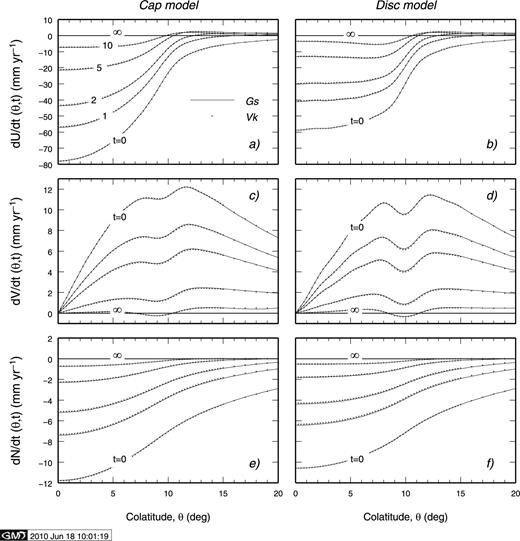
Rates of vertical, horizontal and geoid displacements at the Earth's surface (Test 2/2) according to Gs (VNM method, solid lines) and Vk (SFE, dots) for a cap ice-sheet model (left-hand side) and a disc (right-hand side) imposed at time t= 0. Symbol ‘∞’ marking the horizontal lines in each plot stands for t= 10³ kyr.

Open in new tabDownload slide

4.2.3 More results for Tests 1/2 and 2/2

Within the spatial domain tests, we have also provided insight into two further problems: (i) the effective role of harmonic degree one signals in GIA modelling and (ii) the relationship between FEs results and VNM predictions. The outcomes of these analyses are summarized in this section.

To assess the contribution of the harmonic degree n = 1 of the load to the displacement fields, we consider the results in Fig. 11, where vertical (left frames) and horizontal components of displacements and velocities (right frames) are computed, for the cap load, in the reference frame of the CM of the system (Earth + Load). Solid and dashed lines show results obtained including and neglecting the degree n= 1 load component in eq. (17), respectively (dashed lines reproduce the results in Figs 9 and 10). All quantities are presented for times 0, 1 and 2 kyr after loading. SFE results by Vk are shown by crosses. Geoid displacements are not shown since in CM reference frame their harmonic degree 1 component vanishes. This follows from MacCullagh formula (Greff-Lefftz & Legros 1997), which imposes k^L=−1 (see Fig. 8). Including the degree 1 of the surface load produces the maximum effects beneath the load for U, whereas for V the offset between solid and dashed curves increases with colatitude. This pattern is explained by the colatitude dependence of the degree 1 Legendre polynomial and its derivative in the series (17), which varies as cos θ and sin θ, respectively, and can physically be understood as the geocentre motion described by the degree 1 components of the displacement (Klemann & Martinec 2009). The overall effect of degree 1 is to increase U up to ∼10 per cent beneath the load, while the effect upon horizontal displacement is, at the load margins, of comparable amplitude. These estimates are associated with viscosity model employed here (M3–L70–V01) and on the timescales considered. In view of the time dependence of degree 1 Heaviside Love numbers shown in Fig. 8, larger effects are expected for longer timescales, especially for component V, which shows their maximum amplitude for t∼ 100 kyr.

Figure 11

Vertical (a) and horizontal displacements (b) computed for model M3–L70–V01 in the CM frame. VNM predictions by Gs are shown for the case where the degree n= 1 component of the surface load (cap) is included (solid lines) or excluded (dashed). Crosses denote solutions of Vk (SFE method). In the two bottom frames the test is repeated for vertical (frame c) and horizontal velocities (d).

Open in new tabDownload slide

Fig. 12 shows a comparison between VNM computations (Gs) and FE results (Pg and Bl) based on model M03-L70-V01. At this stage of the benchmark activities, we can only provide a study of vertical displacements (U, top) and rates of displacement (, bottom) pertaining to a cap model with a Heaviside time history. Gs computations, shown by solid lines, are truncated at harmonic degree n_max = 72 and do not include the load component of harmonic degree 1. Using a spherical FE realization of M03-L70-V01 which includes the effects of self-gravitation (the approach is detailed in Dal Forno et al. 2010), Pg has provided predictions (shown by crosses) that reproduce the general features of VNM results but slightly underestimate them especially in the early stages of loading. A possible cause is the coarse FE grid spacing in the region beneath the load, which can be improved in further computations. According to previous experience, after tuning these geometrical features of the FE model, an excellent agreement with VNM results is expected, both for non-self-gravitating (Giunchi & Spada 2000) and self-gravitating models (Wu 2004). The FE results provided by Bl (circles) are not expected to match the VNM ones by Gs exactly, since they are based on model M3–L70–V01f (the flat-earth realization of M03-L70-V01), in which self-gravitation is not implemented. Bl results for vertical displacement (a) exceed the ones by Gs beneath the load, and clearly show a lateral fore-bulge of considerably smaller amplitude in the region θ≥ 10°. These results are in agreement with Amelung & Wolf (1994) who compared analytical flat-earth models to spherical models and observed a similar difference in magnitude and sense of the displacements. Schotman et al. (2008) recently compared flat-earth FE models with spherical models and concluded that the difference between the two are larger during loading than during unloading. In the range of times t≥ 1 kyr (b), the three models considered in this test provide comparable results for .

Figure 12

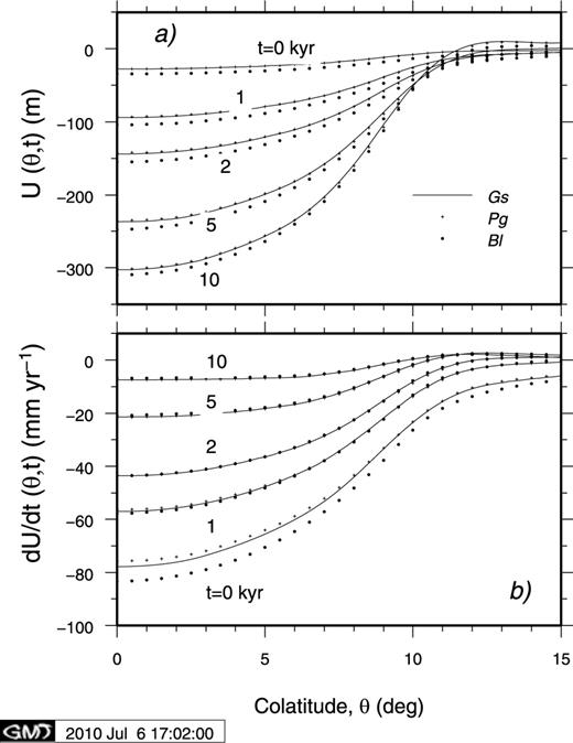
Vertical displacement (a) and rate of vertical displacement (b) computed for Tests 1/2 and 2/2 using two FE implementations of model M3–L70–V01. The first provided by Pg (crosses) is based on an FE spherical model and includes self-gravitation. The second, provided by Bl (dots) is for a flat Earth (M3–L70–V01f). The FE results are compared with the VNM results obtained by Gs. A cap ice model is used.

Open in new tabDownload slide

4.2. Results for Test 3/2 (polar motion and LOD)

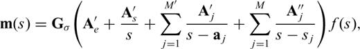
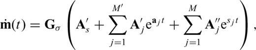
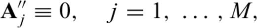
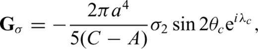
The coefficients A′_s and A′_j that enter the polar motion solution in the time domain (see eqs 28 and 29) are shown in Table 13 according to results provided by Vb and Gs. Results for polar motion in the time domain (Test 3/2) are presented in Table 14. Rather than individual Cartesian components, we provide numerical values of |m| and for various values of t and for the three load models of Table 4. The corresponding geometrical factors G_σ are provided in the table header. Results by Gs include the contributions of the small numerically determined A″_j coefficients in eqs (28) and (29), whereas in computations from Vb the exact algebraic result (eq. 30) is applied. Left- and right-hand parts of Table 14 show results obtained including (Cw ≠ 0) and excluding (Cw = 0) the Cw term from eqs (28) and (29). Since the real parts of A′_s and (A′_j) exceed their imaginary parts by several orders of magnitude (see Table 13), Arg(m) and essentially coincide with ; if Cw ≠ 0, this condition is met after a transient determined by the real part of the rotational mode carrying the Cw (the rotational mode M0, see Table 8 and Vermeersen & Sabadini 1996).

Table 13

Real (top) and imaginary parts (bottom) of constants A_s and A′_j (in units of kyr⁻¹) provided by contributors Vb and Gs. In the numerical computations by Gs, upper bounds on the moduli of coefficients are |Re(A″_j)| ≤ 10⁻⁶ kyr⁻¹ and |Im(A″_j)| ≤ 10⁻⁵ kyr⁻¹ for all rotational modes, while according to Vb the algebraically exact result holds.

Open in new tabDownload slide

Table 14

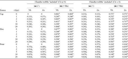
Solutions of Liouville equations for polar motion and the rate of polar motion for Test 3/2. Three ice load models are employed, with corresponding geometrical factors G_cap=−(0.541₄+ i 0.202₃), G_disc=−(0.539₄+ i 0.201₃) and G_point=−(0.152₄+ i 0.570₄). The cases Cw ≠ 0 and Cw = 0 are separately considered. Numerical values are obtained by truncating the outputs provided from Gs and Vb to three significant digits. Some of these solutions are displayed in Fig. 13.

Open in new tabDownload slide

The two time domain solutions of Table 14 differ in several aspects. The one with Cw ≠ 0 (left) obeys the initial condition m(0⁺) = 0 (see eq. 9), whereas the one with Cw = 0 (right) contains, at t= 0, an elastic contribution determined by A_e (see eq. 28). Furthermore, because of the high frequency of the Cw, for Cw ≠ 0, we observe large rates of excursion of the pole of rotation, which approaches the Cw = 0 results only after a few kyr (the decay time of the Cw is, for model considered here, of the order of ∼1 kyr according to Table 8). These marked differences between the two solutions are not in contradiction with the argument of Section 2.1, where Cw effects are argued to be negligible in GIA studies. In fact, the solutions of Table 14 pertain to a Heaviside loading, whose ‘characteristic period’ is vanishingly small compared with both the GIA and the Cw timescales. Using a smooth load history, with a characteristic timescale of a few thousands of years (typical of GIA), would prevent this abrupt excitation of the Cw. The agreement between the contributions of Vb and Gs in Table 14 is satisfactory. However, some mismatch is observed for small times in the case Cw ≠ 0 (see left part of the table). One reason may reside in the small differences in the A′_j coefficients determined by the two contributors and particularly in the terms corresponding to the Cw (see Table 8). Another possible source of error is the numerical noise introduced by the A″_j residues, which are computed and included in the expressions (28) and (29) by Gs, while Vb uses the analytical result (eq. 30).

In frames (a) and (b) of Fig. 13, the two solutions considered in Table 14 are compared to gain more insight into the time evolution of m (expressed in degrees) and (degrees per Ma). Only solutions corresponding to the ice cap model are shown. The solid curves have been obtained by Gs using code PMTF while points along the curves correspond to benchmark calculations by Vb also based on the results of Table 14. From frame (a) it is apparent that solutions with Cw = 0 physically correspond to the time average of those with Cw ≠ 0 and match when the Cw has been completely damped (this occurs after ∼4 kyr in this case study). The rate of polar motion, shown in frame (b) in the case Cw = 0, attains its largest amplitude at the time of loading and decays exponentially to values close to 1° Ma⁻¹ after ∼5 kyr. According to eq. (29), the asymptotic limit is , which is consistent with the linear trend of visible in frame (a) after the initial transient.

Figure 13

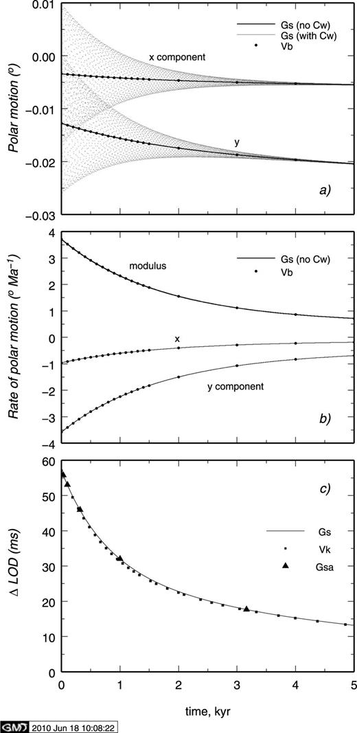
Polar motion (a), rate of polar motion (b) and LOD variation (c) computed for model M3–L70–V01 (Test 3/2). In all computations, a cap surface load is assumed.

Open in new tabDownload slide

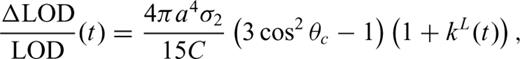
In Fig. 13(c), the variation of LOD, ΔLOD, is shown as a function of time. Solutions for 1 +k^L(t) provided by Gs, Vk and Gsa in the time domain for Test 5/1 (see Section 4.1.5) have been rescaled by Gs using eq. (33). The results for ΔLOD are shown in units of ms (milliseconds) assuming LOD = 86 400 s. The positive values of ΔLOD indicate that the total inertia variation ΔI_zz driven by the load is producing an increase of the LOD relative to the reference value. In the fluid limit (t↦∞), these perturbations will not vanish since at harmonic degree 2 the isostatic condition 1 +k^L(t) = 0 is not attained because of the presence of the elastic lithosphere (for a discussion see e.g. Ricard et al. 1993). The three solutions shown Fig. 13(c) are matching to within ±2 ms, a small discrepancy that can be attributed to the approximations imposed by the spatial discretization (Vk) or to the number of significant digits employed in modelling (Gs and Gsa).

5 Discussion and Conclusions

The analysis of spectral quantities in Tests 1/1 to 3/1 has shown a general agreement between the results obtained. Though the determination of the isostatic spectrum of relaxation is not a straightforward exercise and the numerical implementation of the VNM method differs between contributors, the results for loading and tidal Love numbers agree to a very high precision (at least to within one part in 10³) up to degree 128. Differences in the outputs between ‘competing’ VNM codes (namely Gs and Vb) are more significant in the case of the rotational response (see Test 4/1). The reason ultimately resides in the wide range of timescales involved, ranging from the ‘fast’ Chandler oscillation (period of ∼1 yr), to those associated with the rotational M-modes (∼10⁶ yr). The resulting stiffness and possibly the propagation of errors in the handling of large-degree polynomials makes the model outputs quite sensitive to the settings of the algorithms employed (e.g. complex polynomial root finding) and to the precision allowed in computation. As shown explicitly for model M3–L70–V01, these factors may produce sensible differences in the PMTF coefficients, which however only affect the rotational modes with small strength. Since we could not extend the rotational analyses to more complex models, the general validity of these observations is difficult to establish. From the work done, however, we confirm that the determination of the rotational spectrum is indeed a challenging problem, but it can be significantly alleviated by cross checking and collaboration.

Results from Tests 5/1 to 7/1 are particularly valuable, since these tests have been tackled by at least three contributors, who provided computations based on a wide spectrum of independently developed methods. In the relatively straightforward case of model M3–L70–V01, characterized by a limited number of layers hence by a relatively simple spectrum of relaxation, it has been possible to find a satisfactory agreement between time-domain Love numbers computed by VNM, Post–Widder inversion formula and SFE. Remarkably, after tuning of the numerical codes involved, the same level of agreement between the numerical outputs has been verified also using a complex multistratified model with a non-monotonous viscosity profile (VSS96), in spite of the rich spectrum of relaxation timescales that can make it difficult to ‘follow’ the interlacing branches of the relaxation diagram (i.e. to resolve individual modes) with increasing harmonic degree. The computation of harmonic degree 1 Love numbers is necessary to refer unambiguously geodetic quantities to the CM frame (Blewitt 2003). Through Test 7/1, five contributors have provided an agreed set of loading Love numbers for this degree, on a broad time range and a set of viscoelastic residues determined by VNM. Although the physics of degree 1 Love numbers was established long ago (Farrell 1972), some of the workers contributing to this test (e.g. Gs) have been forced to update their own codes in view of the special boundary conditions demanded by degree n= 1 Love numbers (Greff-Lefftz & Legros 1997). The achieved agreement between the various predictions is the pre-requisite to the SLE benchmark that the COST ES0701 community is undertaking and for a correct interpretation of geodetic observations (e.g. GPS data) in terms of GIA.

Spatial domain Tests 1/2 and 2/2 have tackled by VNM, SFE and FE techniques. Although the agreement between VNM and SFE has been clearly established in both tests, FE solutions still diverge slightly though they clearly provide a pattern of deformations that reproduces those obtained by VNM. We do not have any evidence that this mismatch is due to some fundamental problem with the FE method; rather, on the basis of previous experience (Giunchi & Spada 2000; Wu 2004), we consider that these problems may be overcome by an improvement of the geometrical features of the integration domain. At this stage, from the results displayed in Fig. 12, we can conclude that (incompressible) FE and VNM (SFE) implementations available within the WG4 community are in agreement to within ∼± 10 per cent if we are concerned with vertical motion, where this error bar cumulatively reflects grid effects and the lack of important physical ingredients in modelling (Earth sphericity and self-gravitation of the solid Earth). The success of the third spatial domain test (Test 3/2) has demonstrated that the polar motion problem can be successfully approached numerically once the general features of the theory are clearly stated and agreed. Though the traditional VNM method used by Gs and the analytical implementation of Vb differ in some aspects, as discussed in the body of the manuscript, the results illustrated in Fig. 13 show a complete physical equivalence both in terms of polar motion and LOD variations.

From above, we can draw the main conclusion that the analytical, semi-analytical and numerical codes employed here to model the GIA problem provide results that are largely consistent and that the differences are sufficiently small such that they can be ignored both in the spectral and in the time domain. Achieving this result has required a considerable amount of work from all the contributors. In some cases, the available codes were oriented to complex applications and not immediately suitable for elementary tasks as those proposed here. In some other cases, individual workers have developed new numerical tools from scratch, which have been validated by others. The outcome of this activity has been a general improvement of the methods, which is a fundamental requisite for our collaboration and for the geophysical community.

The results obtained by various contributors have been compared and discussed, but by no means we have identified ‘preferred’ or ‘reference’ results. Rather, the purpose of intercomparisons was to define an interval that could contain, with some degree of confidence, the ‘true’ solutions to the test problems. Indeed, this could be possible in some important cases (see, e.g. the time-domain Love numbers considered in Tests 4/1 to 7/1), where at least three solutions have been contributed, based on fully independent methods. When only two solutions have been proposed (see, e.g. Test 4/1), it is our opinion that some more tests should be performed before full confidence in the results can be achieved, even if their match appear satisfactory at a first glance. In the future, further tests will be made available to the community via the web by this COST collaboration or, hopefully, can be submitted by other investigators. In this respect, one major field of investigation will be the response of layered viscoelastic compressible earth models, whose theoretical aspects have been a subject of debate in the past (Han & Wahr 1995). Though some contributors (Rr and Vk) have submitted outputs for compressible models, the results are still significantly divergent and demand a thorough reanalysis, also in view of recent results (Cambiotti et al. 2008; Cambiotti & Sabadini 2009).

We believe that the results presented in this study will be of some benefit for the GIA community and, specifically, for scientists approaching the study of GIA for the first time. This is coherent with the rationale of all previous benchmark studies on the same topic that, unfortunately, did not reach the final stage of reporting results. Beside these important pedagogical aspects, this work has already provided a number of tangible benefits for the scientists involved. In fact, during the various stages of the benchmark activities, the contributors have had the opportunity of (i) addressing previous misunderstandings about the GIA theory, (ii) correcting subtle mistakes in the numerical implementation of the theory, (iii) improving existing numerical algorithms and (iv) developing original analytical and numerical techniques. Since some of the participants make their codes publicly available (though the documentation is sometimes missing or poor), we believe that these significant improvements of theoretical and numerical aspects of the GIA research may also have a significant impact on the scientific community.

Acknowledgments

Most of this work was supported by COST Action ES0701 ‘Improved Constraints on Models of Glacial Isostatic Adjustment’. We are indebted to all the Working Group 4 (WG4) members of COST Action ES0701 (http://www.cost-es0701.gcparks.com/) for a number of discussions that have helped to improve the manuscript and to the promoters of previous GIA benchmarks that did not reach a publication stage (see Introduction). Niki Evelpidou is acknowledged for providing advice and for supporting the benchmark activities. We thank Florence Colleoni for very helpful advice and discussions during the preparation of the manuscript. We also thank two anonymous reviewers for their very constructive suggestions and Isabella Velicogna as Editor. The figures have been drawn using the GMT public domain software (Wessel & Smith 1998). The development of code VILMA employed by Vk has been supported by the DFG Priority Program SPP1257. ALMA and TABOO have been developed by Giorgio Spada and coworkers under the auspices of PRIN 2004 and PRIN 2006 grants of MIUR, the Italian Ministry of the Instruction, University and Research. Matt King was partly funded by NERC grants and a RCUK fellowship. Zdenek Martinec acknowledges support from the Grant Agency of the Czech Republic through grant No. 205/09/0546. Giorgio Spada acknowledges the ice2sea project, funded by the European Commission's 7th Framework Programme through grant number 226375 (ice2sea manuscript number 012).

References

Author notes