The maximum likelihood dating of magnetostratigraphic sections

Summary

1 Introduction

The main geomagnetic field is generated in the outer core by processes so complex that mathematical modelling of them is still rudimentary. Almost all our knowledge about field behaviour comes, therefore, from observations. Direct observations spanning the past few centuries can be extrapolated over many million years in the past using the remanent magnetization acquired by rocks during or soon after their formation. The magnetic field observed near the Earth's surface is of the poloidal type, and may be described by the scalar potential expanded in spherical harmonics. This expansion can be interpreted in terms of (apparent) equivalent sources located at the Earth's centre; in particular, the first term of the expansion is associated with an axial dipole. The magnetic record in rocks shows that in the geological history there have been long periods when the first term with stable sign dominated the above expansion, alternating with relatively short periods of instability in the geomagnetic field, possibly resulting in a change in the sign of this term (cf.Merril et al. 1998). This sign represents the polarity of the geomagnetic field, and by convention, the present-day negative sign is regarded as normal polarity. For the purpose of this paper, other basic terms are defined as follows: The time interval between two successive polarity reversals, being much longer than the reversals themselves, is referred to as a polarity interval; a stratum of a sedimentary section that acquired its remanent magnetization during one polarity interval is called a polarity zone; and the boundaries between successive polarity zones are termed geomagnetic polarity reversal horizons.

Each of the above-mentioned horizons represents a surface of approximately constant age in stratified rocks all over the world. Because of this importance for stratigraphy, first recognized by Khramov (1958), all information concerning reversal history has been periodically analysed and incorporated into a consistent system; the present-day version is given by the Geomagnetic Polarity Time Scale 2004 (GPTS 2004) (Gradstein et al. 2004). The chronologically arranged list of polarity reversals is particularly complete over the last 165 Ma, because it is based on magnetic anomalies detected in the oceans by seaborne magnetometer surveys and interpreted to be due to polarity intervals recorded in the volcanic rocks of a steadily spreading ocean floor. This long and continuous record has been calibrated, for example by correlation to many short records accessible on land whose stratigraphic ages are known or that have been dated absolutely. Having been calibrated, this record provides a template against which polarity zones found in sedimentary or volcanic sections can be identified. This identification represents only a final step taken in the stratified rock dating procedure known as magnetic polarity stratigraphy (MPS), usually referred to as magnetostratigraphy, for short.

A time difference between the formation of rocks and the acquisition of their primary remanent magnetization should be mentioned in this context. In the case of the detrital remanent magnetization (DRM), which is one usual type studied by the MPS, magnetic grains with their magnetic moments, aligned once to the ambient magnetic field, may become realigned by the action of bioturbation or other disturbances until their orientations are ‘frozen’ in the process of sediment consolidation. This post-depositional remanent magnetization (pDRM) is expected to be dominant in deep-sea sediments, which are the rocks most convenient for magnetostratigraphy (Kent 1973). To assess the above delay, the Matuyma–Brunhes boundaries observed in sections that differed in sedimentation rates have been compared with astronomically forced cycles of oxygen isotopes. This way, deMenocal et al. (1990) found that the process of consolidation took place about 0.16 m below the sediment surface, whereas Tauxe et al. (1996) assessed this depth as being only a few centimetres. To deduce the time delay, this ‘lock-in depth’ must be divided by the instantaneous sedimentation rate. A special attention must be focused on the possibility of the diagenetic overprint or partial remagnetization, which processes may produce strongly delayed records of the reversal sequences, especially in continental sediments.

The prevailing opinion on the relationship of MPS to other dating techniques may be expressed as follows: It is essential to have some biostratigraphic constraints on the polarity zone pattern resolved from any given section to propose a non-ambiguous correlation to the reference geomagnetic polarity timescale (Gradstein et al. 2004). Having roughly determined the age of a section by biostratigraphy, we can repeat section sampling in search of specific polarity reversal horizons, progressively constraining their levels, until the result seems satisfactory. However, this economical strategy is useless if uncertainty about the age spans many polarity intervals. In this case, section sampling and identification of the detected polarity zones are two strictly separated procedures. The former should be performed with an almost constant sampling interval depending on the supposed sedimentation rate, and the latter, to be objective, may be carried out by an algorithm. This algorithmic procedure is the focus of this paper.

Some authors (Lowrie & Alvarez 1984; Langereis et al. 1984) have identified sequences of polarity zones against that of polarity intervals by means of a cross-correlation between these sequences. However, as Opdyke & Channel (1996) observed, the applicability of this procedure is confined to cases of fairly constant sedimentation rate. Recently, I have shown (Man 2008) that, when the impact of variable sedimentation rate is reduced by a transform incorporated into a flow chart before cross-correlation, polarity zones may be reliably identified under more general conditions. This paper deals with the same topic from another point of view: Theoretically, the most general approach to identification should be based on the Bayesian inference, employing both the above-mentioned prior knowledge and the information resulting from the palaeomagnetic observations themselves. In practice, however, the prior information can be hardly expressed in terms of probabilities. Instead, the polarity zones are identified only against a selected part of the GPTS and all possible patterns drawn from this part of the GPTS are considered with equal prior probability. For example, this selected part never includes the cretaceous superchron. This way, the Bayesian inference is reduced to the maximum likelihood method.

The likelihood function is to be inferred from a stochastic model of the formation of sedimentary sections. Sedimentologists sometimes use these models to study some features of sedimentary sections; an account of earlier results in this respect was given by Strauss & Sadler (1989). It is widely accepted that … stratigraphic sections result from a succession of depositional increments and erosional decrements … As a consequence, these sections record Earth history in two formats: truncated depositional increments (beds), which record part of some episodes of deposition, alternate with surfaces of hiatus. The surfaces of hiatus are the only record both of episodes of erosion or nondeposition and these episodes of deposition whose sediments are eroded subsequently… (Strauss & Sadler 1989). The events of erosion or non-deposition appear to be well documented in sedimentary sections; even the basic units of sedimentary geology are defined in these terms (Campbell 1967). From this point of view, sedimentary sections are much like a recorder tape moving forward and backward by chance, either writing or erasing a record, and confining any statistical inference to the preserved parts. On the other hand, the palaeomagneticians often interpret the results of magnetostratigraphy as if the sedimentation rate were almost constant (e.g. Lorio et al. 1998). The stochastic model given later has the ambition to put these seemingly contradictory concepts together. The choice of this stochastic model may be, however, controversial. Although distributions in statistical physics, for example Maxwell's distribution of velocities, are usually derived from natural assumptions leading to simple functional equations, and may be subsequently verified by means of statistical tests using experimental data, in the Earth sciences, by contrast, we often have to adopt a more pragmatic approach due to the enormous complexity and the lack of quantitative data. The model of deposition and erosion described in Section 3 is not very realistic. Strong objections may be raised namely against the assumption of the independence of consecutive section increments and against the assumption of Gaussian distribution of these increments, because some catastrophic events both in deposition and erosion clearly go beyond it. Nevertheless, this choice of the model has led to relatively simple algorithm of identification, whose application gave satisfactory results.

Moreover, for the sake of this simplicity, the deposition history is assumed to be fitted by a single stochastic model, characterized by two constant parameters over the entire section. On the other hand, there is a darker side to the relative simplicity of our assumptions. We cannot expect that the algorithm given herein can be applied generally. Some limitations are discussed in Section 7. For example, long sections can hardly be fitted by a single stochastic model with constant parameters. The application of the algorithm is, therefore, mostly confined to sections of medium length.

2 The Principal Idea

Let us suppose that each of the samples collected from a section is described by its position in the section and by the direction of its primary remanent magnetization.

Using these directions, the set of samples is partitioned into three disjoint classes, assigned to normal, reverse, and intermediate polarities, respectively (Man 2008). Omitting the third class, the remaining samples are arranged in ascending order of their levels. Provided that the isolated samples differing from their neighbours by polarity are also ignored, to avoid short events that cannot be correlated with the GPTS, each pair of consecutive samples of opposite polarities in the remaining sequence brackets a polarity reversal horizon or an odd number of such horizons. In the former case, each polarity zone is represented by at least two samples.

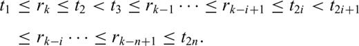
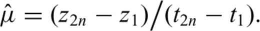
To identify the detected polarity zones, we shall consider only these bracketing samples. Because of the complexity of computations, we could hardly take into account all the samples of the above-mentioned sequence. Moreover, only the positions of the bracketing samples are usually published in digital form. Considering a section where n polarity reversal horizons have been detected, let us denote by z₁ < z₂ < … < z_2n the levels of samples bracketing these horizons. For example, the oldest polarity reversal horizon occurs between levels z₁ and z₂ and the most recent between z_2n−1 and z_2n. Similarly, let us denote by t₁ < t₂… < t_2n the yet unknown times when the bracketing samples have acquired their primary remanent magnetization. Being expressed with respect to the present, these times have the negative sign. The problem to be solved consists in the estimation of times t₁, …, t_2n by comparison of the detected polarity zones with the reference GPTS.

Let us denote by r₁=− 0.781 Ma, r₂=− 0.988 Ma, …, the times of polarity reversals arranged in descending order; if k is an odd or even positive integer, the polarity interval (r_k, r_k−1) has the normal or reverse polarity, respectively.

Provided that no polarity zone has been completely erased by erosion events during the deposition history of the section and all polarity zones present in the section have been detected, there is a one-to-one correspondence between the detected polarity zones and a sequence of equal number of consecutive polarity intervals in the GPTS. In other words, there must be a positive integer k, either odd or even according to the polarity of the zone above the oldest detected polarity reversal horizon, such that the times t₁, …, t_2n satisfy the following inequalities:

1

Inequalities (1) are illustrated in Figs 1 and 2, which refer to actual magnetostratigraphic data (cf.Section 6). These figures show the times t₁, …, t₂₄, satisfying inequalities (1) with k= 39 and 103 respectively, plotted against the levels z₁, …, z₂₄, bracketing the polarity reversal horizons. Whatever times may be chosen, points (t₁, z₁), …, (t₂₄, z₂₄) can be interpolated by a curve representing a possible version of the magnetic record of the section deposition history. For a moment, let us pretend that the times t₁, …, t₂₄ in the above figures have been chosen to make this curve as smooth as possible. Finally, if we compare the versions presented by Figs 1 and 2, the former seems more likely.

Figure 1

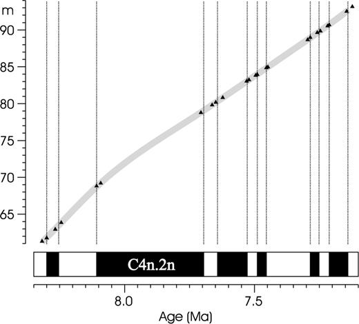
The principle of dating a magnetostratigraphic section. This figure relates the level of samples bracketing the detected polarity reversal horizons (the ordinates of the plotted points) with the possible age of their primary remanent magnetization (the abscissae). The oldest sample acquired its remanent magnetization during a reverse polarity interval, the following two samples during the following normal polarity interval, etc. (cf.Table 1 in Section 6). The times of acquisition were, therefore, constrained by inequalities (1) with the not yet known odd value of index k. We must try all such values and then select the most likely of them. This figure applies to value k= 39. Given this value, we must find the most likely ages subject to constraints (1). The term ‘most likely’ will be specified in the next two sections.

Open in new tabDownload slide

Figure 2

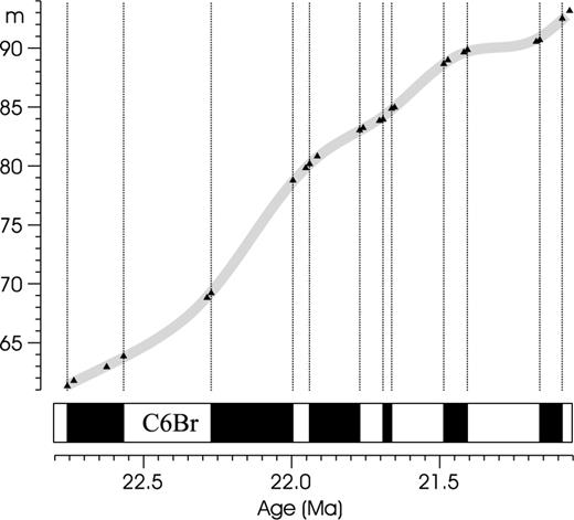
The principle of dating a magnetostrtigraphic section. In contrast with Fig. 1, this one applies to value k = 103.

Open in new tabDownload slide

Below, the intuitive concept of smoothness will be replaced by the likelihood function, defined in terms of probability theory. Nevertheless, the earlier example gave insight into the problem and suggested the following steps for a dating procedure:

• 1

  Using prior information, we choose that part of the GPTS against which the polarity zones are to be identified. This choice and the polarity of the zone above the oldest detected polarity reversal horizon determine the set of possible values for the index k.

• 2

  For each possible value of this index, the likelihood function is maximized with respect to times t_2n satisfying inequalities (1), and with respect to the parameters of the model of deposition. This particular step will be described in detail in Section 4.

• 3

  This way, a value of the likelihood function is assigned to each index k of the above set. If the largest of these values deviates significantly from the average, the corresponding times t1, …, t_2n may be regarded as a solution of the problem. This final step will be discussed in Section 5.

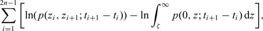
Clearly, the likelihood function depending on levels z₁, …, z_2n, times t₁, …, t_2n, and not yet specified model parameters is a crucial concept of this paper, reflecting the stochastic dependence of the thickness of the polarity zone on the duration of the imprinted polarity interval, which results from the random character of deposition mentioned in Section 1.

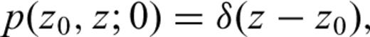
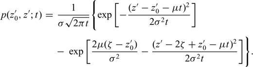
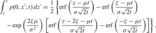
The deposition history of the section is studied, however, through its magnetic record. The relation between these two processes, explained metaphorically in Section 1, is illustrated in Fig. 3. The deposition history may be described by the dependence z(t) of a stratigraphic position z, observed in the compacted section, on the time t of deposition (in intervals where function the z(t) is increasing, that is the instantaneous sedimentation rate is positive) or erosion (wherever this function is decreasing). Obviously, due to episodes of erosion, a particular level z₀ of the section may have been exposed several times in course of deposition history. In other words, equation z(t) = z₀ has not, in general, unique solution. The most recent solution, denoted t₀, is termed the last passage to the level z₀; from this time onwards the erosion base level has never decreased below level z₀. A sample found at level z₀ has acquired its primary remanent magnetization soon after this last passage; the delay depends on the ‘lock-in depth’ modified by the sediment compaction and on the instantaneous sedimentation rate. In contrast to the deposition history of the section, there are no returns in its magnetic record; instead, this record is discontinuous in time.

Figure 3

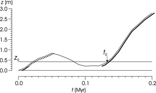
Illustration of the relation between the process of deposition and the magnetic record of this process. The acquisition of the remanent magnetization (the thick line) followed immediately deposition (the thin line), but only the record of the last passage to an arbitrary level of the section has been permanently preserved (the solid line).

Open in new tabDownload slide

In Section 3, the processes of deposition and erosion will be described by the probability that, given its level z₀ at time t₀, the stratigraphic position will achieve level z at time t > t₀. This probability depends on two parameters concerning the sedimentation rate being observed in the compacted section, namely on its mean value and on a parameter quantifying the rate variability. In fact, the above probability is infinitely small, because variable z takes on continuous value; the term ‘probability’ should, therefore, be replaced by ‘probability density’ (cf.eq. 6). In contrast, a magnetic record of the deposition history is described by the probability density which may be derived from the previous one by application of the ‘last passage principle’ (cf.eqs 9 and 13). Finally, in Section 4, using the stochastic description of the magnetic record and turning this problem around, we will identify the probability density of consequent transitions from the state (t₁, z₁) through (t_i, z_i), i = 2, … , 2n-1, to the state (t_2n, z_2n), given the times t₁, …, t_2n and parameters of the stochastic model, as the likelihood of these times and parameters. Unless mathematics is your favourite discipline, you might better skip to Section 5.

3 Stochastic Models of the Deposition History and Its Magnetic Record

Consider the dependence z(t), mentioned in the previous section. We assume that this rather arbitrary dependence obeys some rules of statistical character. These rules define a stochastic process, namely a continuous time-continuous state process, for, being defined for an arbitrary time, it may achieve an arbitrary value. Although its realizations correspond to particular sections, the stochastic process itself is an abstraction representing the common features of all of them. To distinguish between these concepts, the stochastic process and its particular realization are denoted by the symbols Z(t) and z(t), respectively.

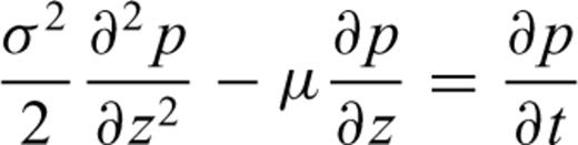
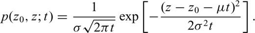
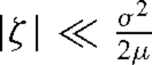
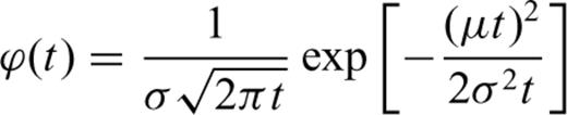
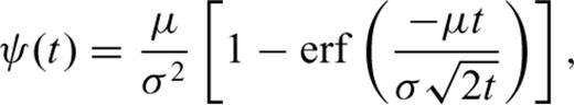
Because of reasons mentioned in Section 1, we assume, along with former studies (e.g. Strauss & Sadler 1989), that Z(t) is a Wiener process with drift μ and variance σ², which means that for any pair t₀, t of time instants satisfying inequalities t > t₀ > 0, the increments Z(t₀) −Z(0) and Z(t) −Z(t₀) are independent, and that for any pair satisfying t > t₀ the increment Z(t) −Z(t₀) is normally distributed with mean μ (t−t₀) and variance σ² (t−t₀) (cf.Cox & Miller 1965). The dimensions of the parameters μ and σ² are length/time and (length)²/time, respectively. Herein, these parameters are considered to be positive constants.

The derivative of the Wiener process is a Gaussian white noise; the realizations of a Wiener process are continuous functions that do not posses a derivative at any point, and, therefore, cannot be plotted. Instead, we can plot the realizations sampled at discrete points. Fig. 4 shows such realizations sampled with a constant sampling rate. The Wiener process was originally introduced to describe Brownian motion and its realizations have been interpreted as particle trajectories.

Figure 4

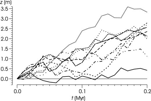
An unrestricted Wiener process with parameters μ= 10 m Myr⁻¹, , satisfying initial condition (5). The realizations sampled with interval 0.01 Myr.

Open in new tabDownload slide

Because of the independence of its increments, the Wiener process is fully described by the transition probability density function (TPDF) p(z₀, t₀; z, t) concerning the probability of the transition from its value z₀ achieved at time t₀ to the value z at time t > t₀. This function is defined

2

the expression on the LHS of this equation is a conditional probability and shall be read as follows: the probability that the process Z(t), starting from z₀ at time t_0, will achieve a value from the interval (a, b) at time t. By its definition, the Wiener process is a time-homogeneous process, which means that the TPDF p(z₀, t₀; z, t) depends on the difference t−t₀ rather than on variables t and t₀ themselves; therefore, this function will be written as p(z₀, z;
t−t₀).

The independence of the increments may be expressed in terms of the TPDF as follows:

3

Moreover, the TPDF may be shown to satisfy the differential equation

4

(cf.Cox & Miller 1965). Each of the eqs (3) and (4), being solved with the initial condition

5

where δ (z) is the Dirac function, give

6

Because this solution is not subject to any boundary condition, the process it describes is termed an unrestricted Wiener process. Stochastic process Z(t) simulating the deposition history of the section is of this type; parameters μ and σ² describe the mean sedimentation rate and the variance of the sedimentation rate, respectively. The assumption μ > 0 means that the deposition prevails over the erosion. The TPDF of this process is plotted by contour lines against variables t and z in Fig. 5.

Figure 5

An unrestricted Wiener process with parameters μ = 2 m Myr⁻¹, , satisfying initial condition (5). Function ln (p(0, z;t)) plotted by contour lines.

Open in new tabDownload slide

The Wiener process Z′(t) simulating the magnetic record of this history, being characterized by the same parameters μ and σ², is, in contrast, restricted by condition

7

resulting from the ‘last passage principle’ mentioned in Section 2. Unfortunately, a non-trivial solution of eq. (4) satisfying conditions (5) and (7) does not exist. However, having replaced condition (7) by a weaker one

8

where ζ < z′₀ is a chosen constant, the solution may be found by the ‘image source’ technique (cf.Cox & Miller 1965) as follows:

9

The process described by this TPDF is termed a Wiener process with absorbing barrier, because it can simulate the Brownian motion of particles that may be caught by a barrier at level ζ. We shall consider the TPDF (9) in the half-plane z′ > ζ only. The integral of this function with respect to variable z′ is given by

10

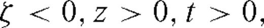whose limit value

11

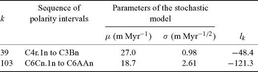
results from the initial condition (5). Particularly, if z=∞, integral (10) describes the probability that the magnetic record will survive the time t. This integral decreases with this time just as the number of particles that have not been caught by the absorbing barrier until time t. Provided that and , this integral reads

12

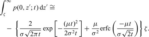
If , expression (9) may be approximated for t≫ (z′₀−ζ)/μ by the following single term of the Taylor expansion with respect to variable ζ:

13

If ζ tends to z′₀, this expression tends to zero uniformly in the half-plane z′ > ζ et al. We shall consider a constant value of the difference z′₀−ζ=ɛ in all equations that include parameter ζ. Function (13) computed for ɛ= 0.001 m is plotted by contour lines in Fig. 6.

Figure 6

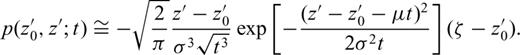
A Wiener process with absorbing barrier ζ=− 0.001 m, parameters μ= 2 m Myr⁻¹, , satisfying initial condition (5). Function ln (p(0, z;t)) plotted by contour lines.

Open in new tabDownload slide

4 The Likelihood Function and Its Maximization

Now, let us come back to the magnetic record described in Section 2. Let us denote by P(z₁, …, z_2n; t₁, …, t_2n, μ, σ) the probability density of the consequent transitions from the state (t₁, z₁) through (t_i, z_i), i = 2, …, 2n - 1 to the state (t_2n, z_2n). Because of the postulated independence of the increments during non-overlapping time intervals (t_i, t_i+1), this function is expressed by the product of factors p(z_i, z_i+1; t_i+1−t_i), i= 1, …, 2n− 1, being given by eqs (9) or (13). The identification of the detected polarity zones requires this function to be maximized with respect to times t₁, …, t_2n subject to constraints (1) and positive parameters μ and σ, given the levels z₁, …, z_2n. In practice, however, it is more convenient to maximize the logarithm of this function

14

Computing function (14) and its partial derivatives with respect to parameters t₁, …, t_2n, μ, σ, we shall always consider the TPDF expressed by approximation (13). Function P(z₁, …, z_2n; t₁, …, t_2n, μ, σ) is herein termed the likelihood function, although some objections to this terminology may be raised because of the time-dependence of integral (12).

Given the times t₁, …, t_2n, equations

15

and

16

have a unique solution with respect to parameters μ and σ², and the negative signs of the second derivatives confirm this solution as the maximum of function (14). If all parameters t₁, …, t_2n, μ, σ are adjustable, their values may be regarded as coordinates of point p in a vector space of dimension 2n+ 2. With the scalar product and the Euclidean norm defined in the usual way, we can express the cosine of the angle between two vectors of this vector space, as well. The domain D of function (14) is a subset of this parameter space defined by constraints (1) and inequalities μ > 0 and σ > 0. Function (14) is supposed to be unimodal in D. An iterative process moves point p within the domain D so that the value of function (14) at this point may progressively increase; if these increments are negligibly small, the process is stopped.

The iterative process starts with an initial guess of parameters chosen as follows: the levels of the detected polarity reversal horizons are estimated by the midpoints h_i= (z_2j−1+z_2j)/2, i= 1, …, n. If these levels are related to the times r_k, …, r_k−n+1 of polarity reversals, the likelihood function depends only on parameters μ and σ, and eqs (15) and (16) yield solution

17

and

18

Finally, these estimates of parameters μ and σ are completed by times t₁, …, t_2n, being chosen so that the resulting point p may be an inner point of domain D.

Each step of the iterative process consists of the following procedures:

• 1

  The computation of gradient g (p) of function (14). The constraints that prevent the point p from moving in the direction of gradient are termed active constraints. The position of the point p with respect to the boundary ∂D of domain D is characterized by a set of active constraints; if p is an inner point of domain D, this set is empty. If the set of active constraints is empty, the feasible direction assigned to point p is given by vector ∂D, otherwise it is given by the projection of this vector onto a part of boundary ∂D being determined by the active constraints.

• 2

  Let us consider a half-line extending in a feasible direction from point p. Point p is moved along this half-line within the domain D so that the cosine of the angle between the current feasible direction and that of the following iterative step may be approximately c, unless the set of active constraints is changed. The value of parameter c decreases in the course of the iterative process from 1 to 0, which strategy prevents the consecutive iterations in the early steps of the process from oscillating.

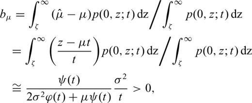
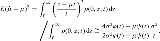
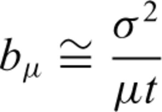
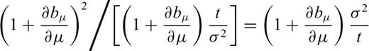
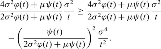
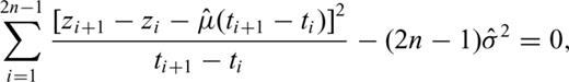
So far, we have only focussed on the numerical aspects of the maximization of function (14). However, what are the properties of the estimators of parameters t₁, …, t_2n, μ, σ resulting from this maximization? It can be shown that the estimators resulting from eqs (15) and (16) are biased and, moreover, the estimator of parameter σ² is inconsistent.

Really, the estimator of parameter μ is

19

Using symbols

20

and

21

the bias of this estimator may be expressed as follows:

22

where symbol t stands for t_2m−t₁. Similarly,

23

The inequality t≫σ²/μ² implies

24

and

25

By means of the last equation, the Binaymé–Tchebyshev inequality reads

26

Finally, we shall examine the efficiency of estimator . The Fisher's inequality reads

27

The RHS of this inequality may be rewritten

28

and the whole inequality may be expressed by means of functions the ϕ(t) and ψ(t) as follows:

29

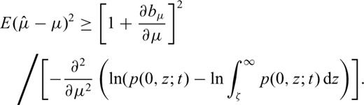
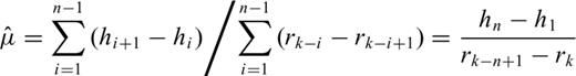
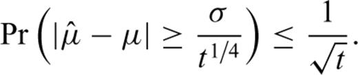
We can conclude that as μ²t/σ²→∞, bias b_μ tends to zero [cf.eq. (24)], the estimate tends to the true value μ in probability [inequality (26)], and the estimator is nearly efficient [inequality (29)]. This result may be translated into comprehensible language as follows: the expected increment in the magnetic record of the section thickness during a long time interval is almost proportional to the length of this interval, especially if the coefficient of variation of the sedimentation rate σ/μ is low.

The estimator of parameter σ² is

30

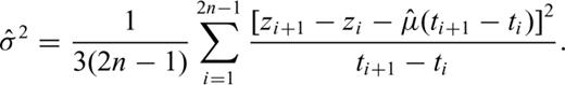
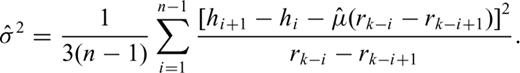
An analysis of its properties is more complicated and shows that . The estimates of parameter σ obtained by the maximization of function (14) will be, therefore, multiplied by the coefficient 1.5.

If the maximized function (14) were replaced with

31

we could expect better results for the estimators at the expense of simplicity of the equations defining them. The simplest form of these equations

32

33

valid when , may be easily solved, but the analysis of the properties of estimators thus obtained is beyond our scope.

5 The Final Step and Test of Significance

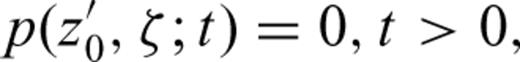
Suppose that a particular stochastic model of deposition described by parameters μ and σ, particular times t₁, …, t_2m satisfying constraints (1), and the resulting value l_k of function (14) have been assigned to each possible value of index k by the constrained maximization of this function. Let us denote the largest of values l_k by l_K. The solution associated with this largest of values l_k, denoted by l_K, most likely corresponds to reality. However, this formal solution need not be always correct. As will be shown in Section 7, the correct solution need not exist at all. If so, we can expect all values l_k, including the largest, to belong to the same distribution. By contrast, if the solution corresponds to reality, value l_K may clearly deviate from the cluster of remaining values. Therefore, being unable to test the hypothesis that the identification failed, we shall test the null hypothesis that all values l_k are drawn from the same distribution, against the alternative hypothesis that one of these values, namely the largest, deviates from this distribution. The null hypothesis is denoted by the symbol H₀.

Values l_k except the largest being regarded as samples of the unknown distribution, the test is based on the sample mean and the sample standard deviation, denoted by the symbols m and s, respectively. We shall, certainly, reject hypothesis H₀ if the statistic (l_K−m)/s is high, namely, if it exceeds some critical value u. This critical value of the test is usually chosen so that the probability of rejection of a true hypothesis may not exceed the chosen significance level α. This probability, however, is given by the LHS of the Bienaymé-Tchebyshev inequality

34

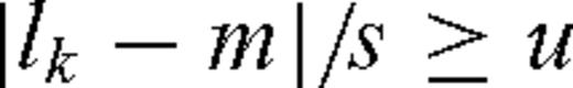which shall be read as follows: the probability that, if hypothesis H₀ is true, it applies . The RHS of this inequality should equal the chosen significance level α and so α= 0.05 implies u = 4.47. Therefore, if it holds that

35

hypothesis H₀ must be rejected at significance level of 0.05 and the identification of polarity zones is to be accepted; in the opposite case we cannot rely on the result of the identification, although it may be correct.

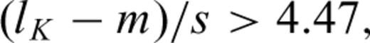
In this section we focused only on the mathematical formalism of testing the significance of the solution. We have made it clear that the result of the identification cannot be regarded as reliable, unless the statistic on the LHS of inequality (35) exceeds some critical value. The conditions affecting this statistic will be discussed in Section 7.

6 Applications

The described algorithm has been tested by application to various published magnetostratigraphic data, referring to sections where traditional dating provided a term of comparison. The prior knowledge concerning the section age, that would be certainly used in practice, has been, however, almost completely ignored and the published polarity zones have been identified against either the C-sequence or the M-sequence of polarity intervals given by the GPTS 2004, to prove that the dating based purely on the magnetostratigraphic data may be possible. If we took the advantage of the prior information, identifying the polarity zones against a shorter sequence of polarity intervals, the probability of a correct result could not be lower.

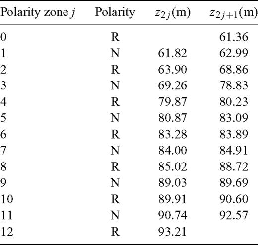
Here, we focus namely on the section Metochia, Gavdos, Grece (Krijgsman 1996). The magnetostratigraphic data describing this section were published exactly in the form required by the above algorithm. In fact, this algorithm was applied to part of this section only. Had the full range of the section been considered, the problem would have been oversimplified. Moreover, the deposition of short sections is more likely to be fitted by a single stochastic model. The sequence of 11 complete polarity zones included in Table 1 was identified against the C-sequence of polarity intervals except for the superchron C34n. Because of the normal polarity of the zone above the oldest detected polarity reversal horizon, only the odd values of index k in the inequality (1) were taken into account, namely k = 11, 13, . . . , 187. With each of these values substituted into constraints (1) function (14) was maximized with respect to parameters t₁, …, t₂₄, μ, σ; the resulting values l_k are plotted against index k in Fig. 7.

Table 1

Input data: the polarities of zones and the levels of samples bracketing the polarity reversal horizons.

Open in new tabDownload slide

Figure 7

The maxima of the likelihood function with respect to parameters μ, σ and times t₁, …, t₂₄ subject to constraints (1), plotted against index k. The thick line denotes a 95 per cent confidence limit for the likelihood function. Symbols m and s were defined in Section 5.

Open in new tabDownload slide

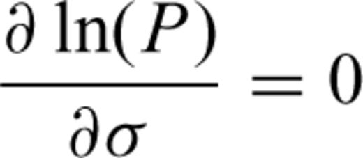
Finally, this set of possible solutions was arranged in the descending order of values l_k; the leading items of this list are given in Table 2. Now, we may reveal that Figs 1 and 2 correspond to the solutions shown in this table. The levels z₁, …, z₂₄ have been drawn from Table 1 and times t₁, …, t₂₄ have, in fact, been obtained by the maximization of function (14). Functions (13) describing the corresponding stochastic models are plotted by contour lines in Figs 8 and 9, together with pairs of differences (t_i+1−t_i, z_i+1−z_i), i= 1, …, 23. Although the level differences z_i+1−z_i, resulting directly from the input data, are common to both figures, time differences t_i+1−t_i, being deduced from different constraints (1), are different. You can sum the logarithms of function (13) over the above pairs to confirm the values ln(P) shown in Table 2.

Table 2

The results of maximization of function (14) with respect to times t₁, … t₂₄ subject to constraints (1) and with respect to parameters μ, σ of the stochastic model of deposition; the achieved maximum depending on index k is denoted by symbol lk et al. The list of results is arranged in descending order of values lk and confined to two leading items.

Open in new tabDownload slide

Figure 8

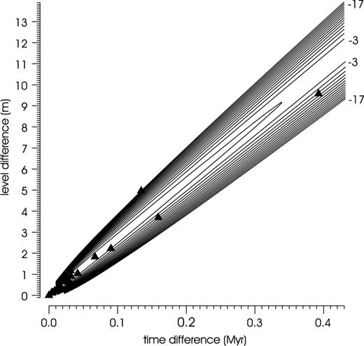
Function ln (p(0, z;t)) describing the stochastic model of the magnetic record of deposition history associated with index k= 39, plotted by contour lines together with pairs of differences (t_i+1−t_i, z_i+1−z_i),i= 1, …, 23.

Open in new tabDownload slide

Figure 9

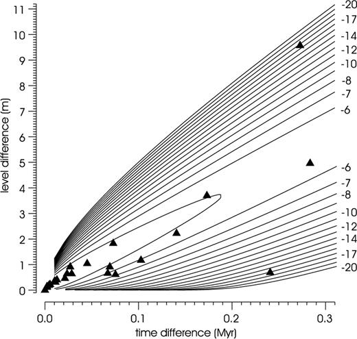
Analogous to Fig. 8, applies to index k= 103.

Open in new tabDownload slide

The statistic on the LHS of inequality (37) takes value 5.73; the possibility that the results associated with the largest of values l_k are insignificant must be, therefore, rejected at significance level 0.05. Actually, times t₁, …, t₂₄ shown in Table 3 are in agreement with the former dating by biostratigraphy and cyclostratigraphy. The stochastic model of deposition associated with the largest of values l_k is characterized by a low value of the coefficient of variation of the sedimentation rate, which is a rather common case, perhaps because the magnetostratigraphy is preferentially applied to sedimentary sections of this type.

Table 3

The estimated ages −t₁, ..., −t₂₄ of the primary remanent magnetization of samples bracketing the polarity reversal horizons, related to the sample levels z₁, …, z₂₄ and the nearest polarity reversals r₃₉, …, r₃₉.

Open in new tabDownload slide

With only one exception which will be discussed in Section 7, all magnetostartigraphic sections considered have been correctly identified either against the C-sequence (except of the superchron C34n) or against the complete M-sequence of polarity intervals given by the GPTS 2004. These results are summarized in Table 4.

Table 4

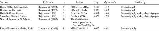
Summarized results of application of the algorithm to several published magnetostratigraphic sections. The symbols used in the column heads were introduced in Sections 2, 3 and 5. The polarity zones were identified with the sequence pattern of polarity intervals.

Open in new tabDownload slide

7 Limitations to Applicability

The following conditions make the identification of the detected probability zones against the GPTS impossible:

• 1

  The data do not reflect all the polarity intervals given by the GPTS either due to a hiatus in the sedimentary section or because of incomplete sampling. The data may also include an excessive polarity zone due to a short-time event not included into the GPTS.

• 2

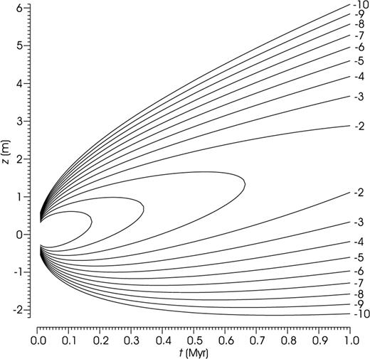
  Because of suddenly varying conditions, the entire section cannot be fitted by a single stochastic model of deposition. As an example, Fig. 10 shows a section that may be piecewise fitted by two very different stochastic models of sedimentation alternating with each other.

Figure 10

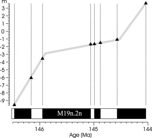
Demonstrating the section Nordvik (Houša et al. 2007). The dating is based purely on biostratigraphy, the polarity zones could not be identified by the algorithm. The levels of polarity reversal horizons plotted against the corresponding times of polarity reversals show that the deposition of this section cannot be fitted by a single stochastic model.

Open in new tabDownload slide

In most cases, the identification is possible in principle, but the reliability of the result depends on parameters of the stochastic model fitting the sedimentary section, on a sequence S′ of polarity intervals that has been imprinted on this section, especially on the number of polarity intervals it included, and on the sequence S⊃S′ of polarity intervals against which the imprinted polarity zones are identified. The impact of these conditions may be studied by means of synthetic magnetostratigraphic sections. Considering a concrete stochastic model of deposition and a polarity interval with duration t, we can use integral (10) to simulate a random quantity described by eq. (9), which provides a model for the imprint thickness. Having selected sequence S, for instance, the M-sequence of polarity intervals, and its subset S′, say, polarity intervals M20n.2n to M18r, we can simulate the imprint of pattern S′ on a sedimentary section of given parameters and, subsequently, identify the resulting synthetic section against sequence S. This trial has two possible outcomes: the result is either identical with sequence S′ or differs from it. Among the total number of trials N, the number M of those having a particular outcome is a binomial variate, and therefore the probability of this outcome is estimated by

36

Some results of such numerical experiments are shown in Table 5.

Table 5

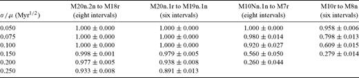
The probability of correct identification of various sequences of polarity intervals imprinted on sedimentary sections characterized by different values of the ratio σ/μ. All imprints have been identified against the M-sequence of polarity intervals. Each probability was estimated using one thousand trials.

Open in new tabDownload slide

The results shown in Table 5 may be commented as follows: The algorithm may be expected to give correct result unless the order relations between the consecutive terms of the imprinted sequence S′ are significantly distorted in the process of deposition. This distortion, however, increases with the coefficient of variation of the sedimentation rate σ/μ, and so does the probability of an incorrect result. For example, the dating of the Bosso Valley section (cf.Table 4) was unreliable (though it was correct) because of a relatively high value of the ratio σ/μ. On the other hand, the impact of the variations in sedimentation rate depends on the variability in duration of the imprinted polarity intervals. If all polarity intervals in the sequence have similar length, even small variations in the sedimentation rate distort the order relations between consecutive terms. The duration of polarity intervals M10Nn.1n to M7r varies only in the range (0.31 Myr, 0.43 Myr) and, therefore, the probability of incorrect identification of their imprint is much higher than that of polarity intervals M20n.2n to M18r, whose duration ranges from 0.05 to 0.88 Myr. These two examples likely represent extreme cases. However, eight seems to be the least number of polarity zones to be reliably identified against either the C-sequence or the M-sequence of polarity intervals even under the most convenient conditions.

8 Conclusions

Let us think of the dating of sedimentary sections in terms of Bayesian inference. Prior information concerning the section age is given, for example by biostratigraphy, while the likelihood function results from the polarity of the primary remanent magnetization of the collected samples. The samples are classified according to their levels and polarities into polarity zones, which are subsequently related to polarity intervals drawn from a template known as the GPTS. So far, it has been widely accepted that this identification is not possible unless the uncertainty left by the prior knowledge is less than 1 Myr, for instance. This paper shows, however, that this uncertainty may be much greater and that sometimes the detected polarity zones may be unambiguously identified even against either the C-sequence or the M-sequence of polarity intervals.

The method described herein uses only those samples bracketing the polarity reversal horizons. Due to the polarities of their magnetization, the ages of this magnetization are constrained by inequalities (1) with not yet known value of index k (Fig. 1). The set of possible values of this index is constrained by the above prior information. Taking the Bayesian approach to its logical conclusion, the likelihood function depending on stratigraphic levels of the bracketing samples, ages of their primary remanent magnetization, and parameters of the model describing the deposition of the section is maximized in two steps. Given a value of index k, it is maximized with respect to the above ages and model parameters; finally, it is maximized on the set of possible values of index k and the significance of this result may be tested (cf.Section 5).

The concept of the likelihood function leads us to the subject of stochastic processes. The process of section deposition, and possibly subsequent erosion, is fitted by a stochastic model characterized by two constant parameters concerning the sedimentation rate, namely by its mean and by a parameter quantifying its variability, whereas the stochastic model fitting the magnetic record of the deposition history may be derived from the former by applying the ‘last passage principle’, illustrated in Fig. 3. The likelihood function is derived from this latter model.

This algorithm was implemented into the program Identification running under MS Windows 32, which is available online at http://www.gli.cas.cz/man/. It was applied to several published magnetostratigraphic sections that included nine or more polarity reversals. With only one exception, these sections were correctly identified against either the C-sequence or the M-sequence of polarity intervals given by the GPTS. These results, summarized in Table 4, may be reproduced using the above program and the attached data files. The conditions making the application of the algorithm impossible or affecting the reliability of the results are discussed in Section 7. One of these limitations requires the deposition history of the section to be fitted by a single stochastic model. A section which does not satisfy this condition is shown in Fig. 10, demonstrating the above-mentioned exception to the successful application of the algorithm. The application, therefore, is mostly confined to imprints of about eight to twelve not very long polarity intervals. Shorter sections cannot be reliably identified without significant prior information, and long sections can hardly be fitted by a single stochastic model with constant parameters.

Acknowledgments

This paper resulted from long-term experience with processing magnetostratigraphic data in the Paleomagnetic Laboratory of the Institute of Geology AS CR, Prague, as part of ongoing research led by Dr. M. Krs and Dr. P. Pruner. In recent years, this research has been supported by the Grant Agency of the Czech Republic (Grant No. GACR 205-07-1365) and by the Research Plan of the IG AS CR No. CEZ AV0Z30130516. The author is indebted to the anonymous reviewers, whose remarks resulted in significant improvements to the paper.

References