


Summary
We determine shear wave splitting parameters of teleseismic SKS and SKKS phases recorded at 43 broad-band seismometers deployed in South Victoria Land as part of the Transantarctic Mountain Seismic Experiment (TAMSEIS) from 2000 to 2003. We use an eigenvalue technique to linearize the rotated and shifted shear wave particle motions and determine the best splitting parameters. The data show a fairly consistent fast direction of azimuthal anisotropy oriented approximately N60°E with splitting times of about 1 s. Based on a previous study of the azimuthal variations of Rayleigh wave phase velocities that show a similar fast direction, we suggest that the anisotropy is localized in the uppermost mantle, with a best estimate of 3 per cent anisotropy in a layer of about 150 km thickness. We suggest that the observed anisotropy near the Ross Sea coast, a region underlain by thin lithosphere, results either from upper mantle flow related to Cenozoic Ross Sea extension or to edge-driven convection associated with a sharp change in lithospheric thickness between East and West Antarctica. Both hypotheses are consistent with the more E–W fast axis orientation for stations on Ross Island and along the coast, subparallel to the extension direction and the lithospheric boundary. Anisotropy in East Antarctica, which is underlain by cold thick continental lithosphere, must be localized within the lithospheric upper mantle and reflect a relict tectonic fabric from past deformation events. Fast axes for the most remote stations in the Vostok Highlands are rotated by 20° and are parallel to splitting measurements at South Pole. These observations seem to delineate a distinct domain of lithospheric fabric, which may represent the extension of the Darling Mobile Belt or Pinjarra Orogen into the interior of East Antarctica.
1 Introduction
Teleseismic shear wave splitting measurements have emerged as a powerful tool for studying the structure and dynamics of the upper mantle because the derived anisotropic parameters are closely related to upper mantle fabrics due to past and present deformation (Silver 1996; Savage 1999). In many cases, the splitting observations can be correlated to the surface geological fabric suggesting that the crust and mantle deform coherently during orogeny as part of the plate (Bormann et al. 1993; Helffrich 1995; Barruol et al. 1997). For example, these studies show that the azimuth of the fast polarization direction is most often parallel to the trend of mountain belts.
Studies of naturally deformed mantle xenoliths (Mainprice' Silver 1993) as well as laboratory studies of artificially deformed olivine aggregates (Zhang & Karato 1995) show that the fast axis of seismic anisotropy is parallel to the extension direction or to the flow direction if there is a distinct flow fabric. Olivine is the dominant mineral type in the upper mantle. It is easily deformable and can develop lattice preferred orientation (LPO) of its crystalline axis (Zhang et al. 2000). This LPO can develop through the active deformation of the asthenospheric mantle associated with absolute plate motion (APM) or could be ‘frozen’ into the mantle lithosphere associated with major tectonic deformational events in the geological past. The orientation of the polarization plane of the faster quasi-S wave in shear wave splitting observations is thus assumed to be a proxy for the orientation of the [100] axis of olivine. This assumption makes it possible to investigate the deformation fabric and possibly the flow direction of the upper mantle.
Due to the harsh conditions of working in Antarctica, which makes operating a seismic station year round difficult, only a limited amount of three-component, broad-band seismological data has been collected. Additionally, splitting observations reported to date (Pondrelli & Azzara 1998; Muller 2001; Helffrich et al. 2002; Pondrelli et al. 2004; Bayer et al. 2007; Usui et al. 2007; Reading & Heintz 2008) consist of stations mainly near the coast or at the South Pole. This study uses data from the Transantarctic Mountain Seismic Experiment (TAMSEIS), the first large-scale, broad-band seismic experiment to reach the interior of the Antarctic continent (Fig. 1), to analyse the seismic anisotropy of the Antarctic lithosphere. These data allow us to determine the geological fabric of the Antarctic interior. Of particular importance is determining the deformation history and mantle flow patterns of the Ross Sea region and the East Antarctic craton where geological data are unavailable. SKS splitting analysis has the potential to delineate different geological terrains and major tectonic boundaries within East Antarctica where ice covers 98 per cent of the surface.
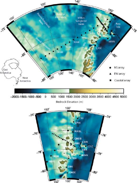
Locations of the TAMSEIS broad-band seismic stations plotted on a map of subglacial bedrock topography (Lythe & Vaughan 2001).
2 Previous Studies
2.1 Regional and tectonic setting
The Antarctic continent has undergone a complex tectonic evolution that is expected to have left some imprints on the lithospheric mantle. Antarctica is generally divided into two major provinces: East Antarctica and West Antarctica (Dalziel 1992). East Antarctica is thought to be a stable continental craton composed of Precambrian metamorphic basement rocks with granitic intrusions that are unconformably overlain by flat-lying sedimentary rocks (Tingey 1991). West Antarctica is an archipelago of microplates with mountainous metamorphic and volcanic terrains (Anderson 1999). The two provinces are separated by the Transantarctic Mountains (TAM). The TAM are an intracontinental mountain belt associated with uplift along the flank of a rift whose boundary follows the front of the range along the Ross embayment (ten Brink et al. 1997). Fission track analysis suggests that the main phase of uplift of the TAM commenced around 50 Ma (Fitzgerald 1992), possibly as a result of rifting and flexure associated with a buoyant thermal load in the mantle beneath the edge of the TAM lithosphere (Lawrence et al. 2006b).
The trend of the TAM is parallel to basement structural features that formed approximately one-half billion years earlier during the Ross Orogeny. The Ross Orogeny formed a Neoproterozoic-to-Ordovician mobile belt along the palaeo-Pacific margin of Gondwana (Stump 1995). It can be described as shortening across a subduction-related volcanic arc system with left-oblique convergence (Paulsen et al. 2004).
The oldest rocks found in the TAM in the vicinity of the TAMSEIS array are 1.7 Gyr old, based on new SHRIMP ion microprobe U–Pb zircon age data for gneissic and metaigneous rocks of the Nimrod Group (Goodge et al. 2001). The regional structural trend of all rocks exposed in the vicinity of the TAMSEIS array, including units that pre-date the Ross Orogen, preserve a pervasive NW–SE fabric related to the Ross Orogeny (Goodge et al. 1991, 2001).
The Pacific margin of East Antarctica has undergone a long history of continental growth and breakup. However, a dearth of geological outcrops on the interior of the continent has led to the conclusion that East Antarctica has remained relatively stable through Phanerozoic time. Consequently, it was initially thought that a single Archaean craton comprises the majority of the East Antarctic lithosphere (Tingey 1991). However, new age data reviewed by Fitzsimons (2003) suggests that one or more Mesoproterozoic-to-Neoproterozoic orogenic belts extend into the interior and divides the East Antarctic craton into separate lithospheric blocks. Another suture has been proposed by Studinger et al. (2003) who suggest that earthquakes in the vicinity of the Vostok highlands may have a tectonic origin. Gravity and magnetic observations (Studinger et al. 2003) as well as the spatial configuration of subglacial lakes on the flanks of the Vostok highlands (Bell et al. 2006) also suggest a compressive tectonic setting for the Vostok highlands region, similar to the Appalachians in North America.
2.2 Previous seismological studies
Continental and global scale surface wave studies (Danesi & Morelli 2001; Ritzwoller et al. 2001) show that the Antarctic crust and mantle are composed of two major geophysical provinces: East and West Antarctica. These results show that the East Antarctic upper mantle is seismically fast, typical of an average continental shield, whereas the mantle beneath West Antarctica is seismically slow, indicative of active tectonism and volcanism. They also suggest that the thickness of the crust of West Antarctica is approximately 27 km, in general, thinner than that of East Antarctica. The East Antarctic crust is approximately 35–40 km thick (Ritzwoller et al. 2001; Lawrence et al. 2006).
More recent results from the TAMSEIS project show that a low-velocity anomaly exists in the upper mantle in the vicinity of Ross Island that extends laterally 50–100 km beneath the TAM (Watson et al. 2006). The depth extent of the low-velocity region is not well constrained but is probably about 200 km (Watson et al. 2006; Lawrence et al. 2006c) Additionally, teleseismic S-wave measurements show that there is greater attenuation beneath the Ross Sea than there is in East Antarctica (Lawrence et al. 2006a), suggesting that the low velocities beneath the Ross Sea result from a thermal anomaly.
Lawrence et al. (2006c) make phase velocity anisotropy observations by comparing Rayleigh wave phase velocities from different azimuths for the central part of the TAMSEIS array. They observe azimuthal phase velocity variations near the intersection of the N–S and E–W arrays with a fast axis of anisotropy oriented between 55 and 85° east of north with a magnitude of 1.5–3.0 per cent. The anisotropy is strongest at periods of 40–75 s but is still visible at periods of 20 and 100 s.
Teleseismic shear wave splitting observations have also been analysed to study the seismic anisotropy of the Antarctic plate at the very northernmost edge of the study region (Pondrelli et al. 2004). They show that seismic anisotropy beneath Northern Victoria Land has a mainly NW–SE fast velocity direction and large delay times of 1–2 s. They suggest this is indicative of a thick, deep-rooted anisotropic layer.
3 Data and Methods
3.1 Data
This study employs horizontal-component, broad-band seismic data recorded at 44 seismic stations (Table 1). This includes 41 temporary stations deployed as part of the TAMSEIS, and three permanent stations with open data access (VNDA, SBA and TNV). The TAMSEIS array consists of three elements (Fig. 1). (1) The ‘North–South’ array—a 1400 km linear array of 17 broad-band seismic stations with 80 km interstation spacing extending from the high central regions of the East Antarctic craton to the TAM. (2) The ‘East–West’ array—an intersecting 400 km linear array of 16 broad-band seismic stations with interstation spacing of 20 km crossing the TAM nearly perpendicular to the first array. (3) The ‘Coastal’ array—11 broad-band stations in the coastal regions along the TAM and on Ross Island. Eight of the stations were installed in December 2000 and the remaining stations were deployed in late 2001, and all stations remained deployed until late 2003. Stations were powered by solar power and batteries during the Austral summer, and employed heating elements to ensure operation in the extreme cold. Stations were shut down by low-voltage and low-temperature disconnects during the winter, such that 5–7 months of data were generally collected each year.

Stacked shear wave splitting results for each station
The events used for this study were required to have a magnitude greater than 5.8 Mw at epicentral distances between 90° and 140°. SKS and SKKS phases were carefully evaluated and those with a sufficient signal-to-noise ratio (SNR) and clearly separated from other phases were chosen for analysis. Most of the data were filtered with a bandpass filter, with a low-frequency corner at 0.02 Hz and a high-frequency corner ranging between 0.2 and 0.5 Hz.
3.2 Shear wave splitting analysis
When an S-wave propagates through an anisotropic medium, it is split into two quasi-S waves with perpendicular polarizations that propagate with different velocities. This anisotropy can be quantified as two parameters: ϕ, the azimuth of the polarization plane of the faster quasi-S wave, and dt, the difference in arrival times between the two split quasi-S waves (Babuska & Cara 1991). The splitting measurements for this study were performed on the core shear phases SKS and SKKS. These phases form as a result of a P-to-S conversion at the core-mantle boundary. The SKS and SKKS phases are polarized in the radial direction and arrive at a station with near-vertical incidence. Thus, the anisotropy measured represents a vertically integrated effect of azimuthal anisotropy from the core-mantle boundary to the surface. However, many studies suggest that the observed anisotropy is concentrated in the upper mantle with possibly small contributions from the core-mantle boundary region (Hall et al. 2004), the crust (Barruol & Mainprice 1993) and the lower mantle.
We determine shear wave splitting parameters using the technique of Silver & Chan (1991). This technique involves analysing the particle motion of each phase by calculating the covariance matrix of the horizontal seismogram components for many possible values of ϕ and δt. The eigenvalues of the covariance matrix are a measure of particle motion linearity. The most linear-restored particle motion, and thus the best parameters for reversing the effect of anisotropy, is found by minimizing the magnitude of the smaller eigenvalue. The splitting parameters reported here are those values of ϕ and δt that provide the most linear restored particle motion. An example is shown in Fig. 2.
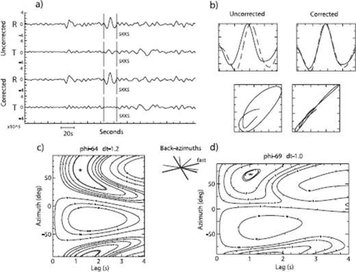
Example of SKS splitting analysis. (a) The horizontal waveforms rotated into the radial and transverse directions. The top two traces show the original rotated traces, whereas the lower two traces have been corrected for anisotropy. Note that the absence of energy on the transverse component on the corrected trace indicates that the splitting parameters used are an appropriate measure of the anisotropy. (b) A close-up of the windowed waveforms and the particle motion plots for both the raw data (left) and the data after correction for the observed anisotropy (right). (c) The contour plot showing misfit as a function of splitting parameters for the event shown in panels in (a) and (b) at station N036. (d) The contour plot for the stacked or global solution.
Individual measurements have been qualitatively rated A, B, C and null based on (1) SNR, (2) linearization of the particle motion and (3) the waveform coherence between the two horizontal components rotated into fast and slow directions. The SNR is defined by the ratio of the maximum amplitude of the radial and the tangential waveforms in the measurement window after correcting for splitting. Measurements satisfy criteria (1) if they have SNR > 4. Measurements that show elliptical particle motion on the uncorrected seismograms and linear particle motion on the corrected seismograms satisfy criteria (2). Coherence between waveforms is determined qualitatively. Measurements that satisfy all three criteria are rated A. Measurements that satisfy two of the above criteria are rated B, and measurements that satisfy only one criterion are rated C. A null measurement does not show energy on the transverse component in the rotated seismograms. This may be due to an absence of anisotropy, an initial polarization of the incoming wave parallel or orthogonal to the fast anisotropic direction, or low SNR. The quality of the data has been visually inspected and only traces rated B or higher have been kept.
To increase the robustness of the results compared to the analysis of single events, we use a stacking method (Wolfe & Silver 1998) to produce a weighted sum of the individual misfit surfaces, and compute an average or global solution for each station. This method also allows efficient use of constraints on the fast-axis orientation provided by null measurements. We use the Restivo & Helffrich (1999) implementation in which individual measurements are weighted in the stack based on the SNR and the back-azimuth to generate the stacked or global solutions. Only individual splitting data with quality A or B are used in the stacking procedure.
The final stacked solutions for each station have been categorized A, B or C based on (1) the back-azimuth sampling and (2) single event rating of the individual data comprising the stack. Stacked solutions with three or more back-azimuth quadrants sampled with single event ratings of A or B are considered robust and are assigned a grade of A. These are plotted as thick vectors in Figs 3 and 4. Stacked solutions with two or more back-azimuth quadrants sampled by single events rated A or B are considered marginally robust and assigned a grade of B. These are plotted as thin vectors in Figs 3 and 4. Additionally, to achieve an A rating, the global solution must consist of at least four individual measurements with one of these four having fast direction greater than 20° away from the back azimuth. This non-nodal measurement must also contain the global solution in the 95 per cent confidence interval. We find that this method of rating is in good agreement with the formal errors reported here. The formal errors are assigned through an F-test analysis according to Silver & Chan (1991).
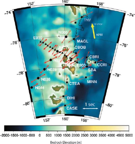
Splitting results in the Trans-Antarctic Mountains and Ross Island region. Azimuth of the vectors denotes the fast direction from the stacked results, and the length of the vector is proportional to the splitting time, with the scale given at the lower right. Thin vectors represent B quality results and thick vectors represent A quality results. The large yellow vector represents the direction of the absolute plate motion.
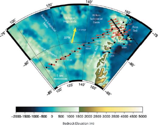
Splitting results across East Antarctica. Thin vectors represent B quality results and thick vectors represent A quality results. The large yellow vector represents the direction of the absolute plate motion.
4 Results
We determine stacked shear wave splitting parameters with a grade of B or better for 36 of 42 stations of the TAMSEIS array plus permanent stations TNV, SBA and VNDA. Six stations collected insufficient data or data of poorer quality, with the stacked data rated lower than B. These results were not used in the subsequent analysis and discussion.
4.1 The Trans-Antarctic Mountains and the Ross Sea coast
The region extending from the Ross Sea across the TAM and into East Antarctica (E–W array) shows a uniform pattern of azimuthal anisotropy within the resolution of the data set (Fig. 3). There is no rotation in the fast direction across the boundary between the TAM and East Antarctica as imaged by aerogeophysical studies (Finn et al. 2006). The average fast direction at the intersection of the N–S and E–W arrays is N58E and is taken from A quality measurements at stations E014, E020, E024, E008, N020, N028 and N036. There is no evidence of any systematic change in the fast direction along the 300 km long dense EW line from the coast across the TAM and into the Wilkes Basin. Stations at Ross Island and some locations along the coast show a more E–W fast direction of anisotropy. The average direction for the Ross Island and coastal stations (excluding CTEA and CBRI) is N67E. CTEA and CBRI show roughly the N–S direction of anisotropy, although these measurements have high uncertainty.
4.2 East Antarctica
Results along the long line of stations extending deep into the interior of East Antarctica are also remarkably uniform (Fig. 4), with the anisotropic direction of all individual station stacks except one between the coast and N060 within 10° of N58E, the average orientation along the central part of the E–W array (Fig. 8). The Belgica Highlands (stations N068-N084) show a consistent clockwise rotation of 15°–20° in the fast direction of anisotropy. Stations N092, N100 and N108, located along lower subglacial topography that represents an extension of the Aurora Subglacial Basin, do not show this rotation. The stations at the far end of the line (N124 and N132) located in the Vostok Highlands once again show a rotation of 15°–20° with respect to the average anisotropic direction of the entire array.
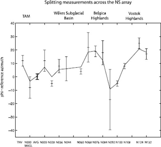
Splitting results for the N–S array plotted as an angle relative to the average splitting orientation near the junction of the N–S and E–W arrays. Error bars denote the 95 per cent confidence interval for the fast direction from the stacked data. The solid line represents a smoothed running mean of the fast direction along the array. Note the highly uniform fast direction in the TAM and Wilkes Basin and the rotation of the fast direction of anisotropy of about 15–20° for stations N068-N084 (Belgica Highlands) and N124-N132 (Vostok Highlands).
Fig. 5 plots the quality A anisotropy results from this study along with results from shear wave splitting studies in other regions around Antarctica. Unlike most other areas, which show fast directions subparallel to the Antarctic margin, fast directions in our study region are oriented at high angles to the continent edge. Fast directions at the end of the line (stations N124 and N132) are nearly parallel with the fast direction observed at South Pole, suggesting they may lie within the same tectonic region within East Antarctica.

Splitting vectors for the entire Antarctic continent compiled from a variety of studies. (Kubo et al. 1995; Kubo & Hiramatsu 1998; Muller 2001; Pondrelli et al. 2004; Bayer et al. 2007; Usui et al. 2007; Reading & Heintz 2008). Results plotted from the TAMSEIS array are limited to A quality observations. Results from other studies are limited to stations with multiple high-quality observations. The grey lines represent a possible extension of Pan-African aged mobile belt into the interior of East Antarctica.
5 Discussion
5.1 Inferred depth of the anisotropic layer
5.1.1 Anisotropy in the crust and ice?
Shallow sources of observed anisotropy may result from the crust and ice layers. However, crustal shear wave splitting measurements are generally on the order of 0.05–0.2 s (Savage 1999), which is much smaller than the average delay time of about 1 s reported in this study. Also, the crustal thickness throughout the region is generally 35 km or less (Lawrence et al. 2006b). Typically, anisotropy in the crust is on the order of 2–4 per cent (Babuska & Cara 1991), so for a 35 km thick crustal layer the expected average splitting time is about 0.3 s. This value is much less than what we observe for most of the TAMSEIS stations.
Ice is also a highly anisotropic mineral that can be aligned by ice flow, and since most of the TAMSEIS seismic stations were deployed on 1–3 km of ice, shear waves could conceivably be split by passage through the ice sheet. Experimental studies for single ice crystals suggest that the difference in shear velocity that might be expected from complete crystal orientation is about 5 per cent (Thiel & Ostenso 1961). However, since the ice layer is on the order of 3 km, we expect the splitting time to be less than 0.1 s, which is insufficient to explain the observations reported here.
Although we cannot completely rule out a small effect of crustal or ice layer anisotropy, they cannot be a major source of the splitting in our measurements. Thus, the large magnitude of the splitting allows us to identify the upper mantle as the primary source of the splitting. This is consistent with other published work, where shear wave splitting times of >0.2 s are usually associated with upper mantle anisotropy (e.g. Silver 1996; Savage 1999).
5.1.2 Depth constraints from previous surface wave results
The anisotropy within East Antarctica just west of the TAM near the junction of the N–S and E–W arrays has an average fast direction of N58E with splitting times of about 1 s. Azimuthal variations of Rayleigh wave phase velocities at the intersection of the N–S and E–W arrays reported by Lawrence et al. (2006c) show a fast axis of anisotropy oriented N65E ± 15° with 3 per cent ± 1 per cent anisotropy. Thus, the fast anisotropy direction determined by surface waves is nearly identical to the average fast direction from this study. The Rayleigh wave anisotropy is strongest at periods of 40 s, but is also detectable at periods ranging from 20 to 120 s suggesting that the anisotropy is located in the uppermost mantle. If we assume that the magnitude of the anisotropy is 3 per cent, as suggested by the surface wave observations, then a depth range extending from 35 to 185 km would be necessary to accumulate the observed splitting magnitude of approximately 1 s. This estimate is consistent with constraints of the anisotropy of continental lithosphere obtained from mantle xenoliths that suggest a maximum S-wave anisotropy (δVs) of 3.7 per cent (Mainprice & Silver 1993). Additionally, this is the same depth where diffusion creep starts to dominate deformation (Karato 1992), and where the olivine c-axis is thought to align in the direction of mantle flow (Mainprice et al. 2005). Both of these mechanisms would act to reduce anisotropy.
We find no evidence of systematic variation in the shear wave splitting fast direction with the back azimuth, as would be expected for two layers with differing anisotropy orientations (Silver & Savage 1994). Due to the short length of the deployment, most stations did not accumulate enough observations with different back azimuths, so we investigated this possible effect with station VNDA, which has been operational since 1994. A grid search for the best-fit two-layer model was performed and it was determined that the solution is non-unique due to the large range of models that suitably fit the data. One such best-fit model is shown in Fig. 6. The data does not fit the curve for a two-layer model any better than it fits for a one-layer model. For example, the two-layer model requires negative fast directions for polarization azimuths between 105° and 125°, and the data do not support this. Additionally, the observed splitting times are much lower than expected for a two-layer model for polarization azimuths between 110° and 150°. Therefore, we conclude that the anisotropy can best be modelled as a single layer in the uppermost mantle.
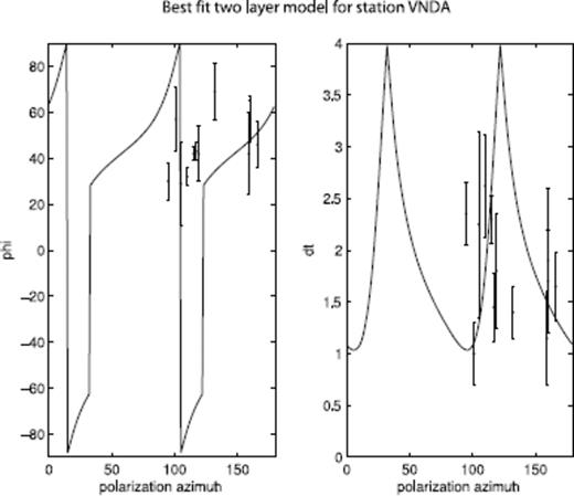
Best-fit two-layer model of anisotropy for station VNDA. The figure shows the splitting function for both the fast direction of anisotropy and the splitting time as a function of polarization azimuth. Layer 1 has a fast direction of 152° with a splitting time of 1.1 s and layer 2 has a fast direction of 44° with a splitting time of 1.7 s. The data points represent the observed data for station VNDA with error bars plotted. Note that the data does not fit the model, especially at polarization azimuths ranging from 105° to 125°.
5.2 Origin of mantle anisotropy in Antarctica
5.2.1 Anisotropy and absolute plate motion
Seismic anisotropy may result from currently active mantle flow, with shear strain and the active olivine slip system producing LPO of the olivine fast axis oriented in the direction of maximum extension that is generally consistent with the flow direction (Ribe 1989). In some cases, mantle flow relative to a continental block may result from APM, or essentially the movement of the continental lithosphere over the ambient mantle (Wolfe & Silver 1998). This hypothesis predicts that the fast anisotropy direction should be parallel to the APM direction. However, the APM of the Antarctic plate in the Ross Sea region is N18W (Gripp & Gordon 2002), inconsistent with the observed splitting results. Additionally, LPO of olivine associated with APM usually only occurs for fast moving plates with a low viscosity zone at the base of the lithosphere (Bokelmann & Silver 2002). The Antarctic APM vector has a magnitude of only 1.3–1.6 cm yr−1 (Gripp & Gordon 2002) making it one of the slowest moving plates on the planet, and unlikely to produce a significant shear strain in the mantle. Additionally, kinematic studies using GPS data indicate that the present-day Antarctic plate motion near our study region is in the southeast direction relative to the International Terrestrial Reference Frame (Bouin & Vigny 2001; Dietrich et al. 2004). This direction is nearly perpendicular to the fast direction of anisotropy observed suggesting that the plate motion and mantle anisotropy are not related.
The shear wave splitting magnitudes combined with the surface wave results (Lawrence et al. 2006c), suggesting that the anisotropy is located in the upper 150–200 km of the mantle, also argue against a present-day mantle flow origin for the anisotropy in the cratonic regions of East Antarctica. Shear strain from mantle flow would be localized within the low-viscosity and high-temperature asthenosphere. However, body wave tomography (Watson et al. 2006) and surface wave phase velocities (Lawrence et al. 2006c) suggest the existence of thick lithosphere down to depths of ∼200 km beneath East Antarctica and extending to the crest of the TAM, in the same region where surface wave anisotropy is observed. Thus, the anisotropic region is observed at depths characterized by cold rigid continental lithosphere that would resist deformation rather than by asthenospheric material with the ability to flow. The lack of shallow asthenosphere makes it difficult to attribute the anisotropy to mantle flow and shear at the base of the lithosphere.
5.2.2 Anisotropy resulting from past orogenic activity
Many active mountain belts have fast splitting directions that are perpendicular to the direction of shortening, indicating that deformation and shortening associated with the orogenic activity produced LPO with the fast direction aligned with the extension axis in the mantle (Silver & Chan 1991; Vinnik et al. 1992). Furthermore, an anisotropic fabric in the mantle lithosphere can remain frozen in for billions of years once the lithosphere cools after such a mountain building event. Continental shear wave splitting studies typically report a correlation between splitting direction and structures at the surface related to the last major deformational event (Helffrich 1995; Vauchez & Barruol 1996; Barruol et al. 1997). They show that the fast direction of anisotropy is typically oriented parallel to the surface fabric. Subcontinental anisotropic fabric can in some cases pre-date the most recent orogenic event if the event did not thoroughly deform the continental mantle lithosphere (Babuska & Plomerova 2006).
One major tectonic mountain building event in the study region that could produce deformation of the lithosphere is the ∼500 Ma Ross Orogeny. This widespread tectonic event is expected to have left an imprint on the subcontinental lithospheric mantle. Structures and fabrics exposed at the surface related to the Ross Orogeny in the TAM are oriented roughly NW–SE (Findlay 1978; Mortimer 1981; Findlay 1984; Allibone 1987; Stump 1995) suggesting a NE–SW shortening direction for the Ross deformational episode.
We report a fast direction of seismic anisotropy oriented roughly NE–SW, perpendicular to the structures exposed at the surface. This would seem to indicate that the anisotropy is not related to deformation occurring during Ross time. Exposures pre-dating the Ross Orogeny are rare in the study area, and earlier units that are exposed have generally been overprinted by Ross structures. For example, rocks associated with the 1.7 Ga Nimrod Orogeny found in the TAM also show Ross fabric oriented roughly NW–SE, overprinting the relict structures from the Nimrod Orogeny (Goodge et al. 2001). All of the structures, lineations, fabrics, etc. that have been mapped at the surface are related to Ross deformation. Since the fast directions we observe are localized to the subcontinental mantle lithosphere but show fast directions inconsistent with the Ross fabric, they may result from structures of different orientation pre-dating the Ross Orogeny. In Europe, observations of consistent anisotropy within individual blocks of the mantle lithosphere reflect frozen-in olivine preferred orientation, most probably formed prior to the assembly of microcontinents that formed the modern European landmass (Babuska & Plomerova 2006).
Additionally, it seems likely that whatever deformational event produced the observed anisotropy in the TAM also produced the anisotropy observed in East Antarctica beneath the Wilkes Basin. This is evident from the continuity of the fast direction of anisotropy from the TAM into the Wilkes subglacial basin (Fig. 7). Furthermore, we do not observe a rotation of the fast axis of anisotropy across the boundary between the TAM and Wilkes basin as defined by aeromagnetic data (Finn et al. 2006). We suggest that the anisotropy is a result of a relic fabric in the cold continental lithosphere that formed prior to the Ross Orogeny.
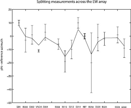
Splitting results for the E–W array plotted as an angle relative to the average splitting orientation near the junction of the N–S and E–W arrays. The average splitting orientation of N58E was determined by averaging the A quality stacks from stations E014, E020, E024, E008, N020, N028 and N036 near the junction of the N–S and E–W arrays. The solid line represents a smoothed running mean of the fast direction along the array. Error bars denote the 95 per cent confidence interval for the fast direction from the stacked data.
5.2.3 Anisotropy and extension in the Ross Sea and TAM front
Splitting observations at Ross Island and along the Ross Sea coast are unlikely to result from frozen-in anisotropy of the continental lithosphere since a cold continental lithosphere is thin or missing (Lawrence et al. 2006; Watson et al. 2006). Instead, anisotropy in this region may result from Cenozoic extension in the Ross sea area. Extension of the mantle lithosphere should produce olivine LPO with the fast axis oriented parallel to the extension direction (Mainprice & Silver 1993). Additionally, shear wave splitting data from some continental rifts, including the Baikal Rift and the Rhine Graben, show fast azimuths parallel to the extension direction (Vinnik et al. 1992; Gao et al. 1997). However, fast directions from other continental rift settings such as East Africa do not match the predicted direction for ductile stretching of the mantle lithosphere (Walker et al. 2004; Gashawbeza et al. 2004).
Tectonic activity in the southwestern Ross Sea and TAM front has primarily involved extension between East and West Antarctica beginning ∼105 Ma and continuing to the present (Lawver & Gahagan 1994; Hamilton et al. 2001). This represents one of the largest active continental rift systems on Earth. Magnetic, gravity and bathymetry data from the Adare Trough allow a pole of rotation to be calculated for East–West Antarctic motion between chron 20 and chron 8, or approximately 43–26 Ma (Cande et al. 2000). This rotation pole suggests a Cenozoic extension direction oriented N85E in the vicinity of Ross Island. The extension direction in the early Cenozoic and Mesozoic is harder to constrain because of a lack of magnetic anomaly and fracture zone constraints on seafloor spreading. In addition, Henrys et al. (2007) infer 10–15 km of post-18 Ma extension along the Terror Rift to the north of Ross Island based on fault displacements. The faults trend approximately N15W, so the inferred extension direction is N75E.
There is some evidence that the fast direction of anisotropy at coastal stations is more EW than is observed at the TAM crest and farther inland where thick cold continental lithosphere is present. The average splitting direction of stations MINN, DIHI, CCRZ, SBA and CASE is 67°, or 10° greater than the average fast direction of 57° reported near the junction of the N–S and E–W arrays. Since these data along the coast are roughly subparallel to the extension direction of N75E inferred from recent terror rift extension, or N85E inferred from the Adare Trough rotation pole, it is possible that Cenozoic extension has stretched the lithosphere in the Ross Sea and is responsible for producing the splitting observations reported in this study.
5.2.4 Asthenospheric mantle flow and edge convection
Active asthenospheric flow induced by large lateral temperature variations at the edge of the East Antarctic craton represent an alternative interpretation for shear wave splitting results in the Ross Sea region. Numerical models demonstrate that small-scale convection develops in the upper mantle beneath the transition of thick cratonic lithosphere and thin oceanic lithosphere (King & Anderson 1998; King & Ritsema 2000). Essentially the edge of the cold rigid continental lithosphere, extending to depths of 200 km, cools the mantle in the vicinity and causes it to sink, causing a small convection cell. The flow direction in the cell will be perpendicular to the edge of the continental craton. Thus, LPO formed by this convection should generally show fast directions that are perpendicular to the edge of the continent.
The splitting parameters reported in this study at stations along the coast (with the exception of CTEA and CBRI that were poorly constrained) record a roughly east-northeast fast axis with the average fast direction of N67E that is a rotation of about 10° relative to observations at the intersection of the N–S and E–W arrays. The edge of the continental craton in this region is roughly N–S, so the predicted fast direction from edge-driven convection is approximately E–W, or subparallel to the observed fast directions. This suggests that the observations along the coast may record a more recent shear fabric oriented E–W, parallel to the minimum strain axes, that is related to a possible current edge-driven convection flow regime.
5.2.6 Splitting directions and possible terrains in East Antarctica
We observe a slight rotation of the fast direction of anisotropy in two highland regions near the end of the N–S array (N132). Fig. 8 shows the fast direction of anisotropy plotted as an angle relative to the average fast direction at a reference location for the N–S array. The results are plotted relative to the reference direction because geographic azimuths change rapidly with longitude near the poles. This figure shows that the splitting results are fairly consistent from the coast (TNV) through the TAM and into East Antarctica as far as station N060 in the middle of the Wilkes Basin. At stations N068–N084 there is a clockwise (positive) rotation of approximately 20° of the fast direction. These stations are located in a highlands region extending southward from the Belgica Highlands. The positive rotation also occurs at the end of the line at stations N124 and N132 in the vicinity of the Vostok Highlands, along with a reduction in the splitting time to 0.5 s, compared to most stations showing splitting magnitudes near 1 s. In between these two regions, stations N092, N100 and N108 along an extension of the Aurora Subglacial Basin have fast directions that are nearly identical to the directions reported near the junction of the E–W and N–S arrays and out to N060. We characterize the two highland regions as a separate anisotropic domain with a smaller degree of anisotropy and a slight rotation relative to the other TAMSEIS stations. This separate domain is located in the vicinity of the highland areas and could represent a major tectonic boundary or boundaries beneath the Antarctic ice sheet.
One such major tectonic boundary might be the Darling Mobile Belt or Pinjarra Orogen (Harris 1994). The Pinjarra Orogen is part of a major tectonic boundary that separates East Gondwana between India and Australia and extends into East Antarctica (Fitzsimons 2003). However, since the geology of this region is buried under ice, the exact path inland is unknown. One model says that it runs westward and intersects the East African Orogen somewhere in Dronning Maud Land (Boger et al. 2001). Another model suggests the Orogen passes through the Gamburtsev Subglacial Mountains and continues on either to the East African Orogeny in Dronning Maud Land or to the Ross Orogen of the TAM somewhere between the Miller and Shackleton ranges (Fitzsimons 2000). If the Orogen extends to the TAM, we might expect to find it under stations located near the end of the N–S array (N132). The change in the fast direction of anisotropy in this region suggests that a major lithospheric boundary is present and may represent the extension of the Pinjarra Orogen. Therefore, our results may record a fast direction of anisotropy associated with the Pinjarra Orogen that extends into and across East Antarctica suggesting East Antarctica is composed of multiple cratonic blocks as opposed to a single cratonic block.
6 Conclusions
We find evidence for a widespread and relatively uniform anisotropic layer in the uppermost 150 km of the mantle beneath East Antarctica just west of the TAM. Our preferred interpretation for these observations is LPO in the upper mantle of the cold continental lithosphere resulting from a tectonic event that predates the Ross Orogeny. Stations along the coast and to the south of Ross Island have a fast direction oriented at N67E, which may be a result of Cenozoic extension between East and West Antarctica that stretched the mantle lithosphere, or the anisotropy could result from active mantle flow in the asthenosphere from edge-driven convection associated with the edge of the cold root of the East Antarctic craton. Observations from the interior of East Antarctica show a 20° clockwise rotation of the fast direction beneath the Belgica Highlands and the Vostok Highlands. These regions may represent separate anisotropic domains within the Antarctic lithosphere, and it is possible that they demarcate previously unidentified tectonic boundaries within East Antarctica.
Acknowledgments
We thank Patrick Shore, Don Voigt, Audrey Huerta, Tim Watson, Bob Osburn, Moira Pyle, Jesse Lawrence, Tim Parker, Bruce Beaudoin, Bruce Long and many other individuals for help acquiring the TAMSEIS data. We thank George Helffrich for use of his shear wave splitting analysis code. We also thank Anya Reading and James Hammond for helpful comments on an earlier draft. Portable seismic instrumentation for this project was obtained from the PASSCAL program of the Incorporated Research Institutions in Seismology (IRIS), and data-handling assistance was provided by the IRIS Data Management System. This research was conducted with support from NSF grants OPP9909603 and OPP9909648.
References
