A comparison of site response techniques using earthquake data and ambient seismic noise analysis in the large urban areas of Santiago de Chile

Summary

1 Introduction

Chile is one of the most seismically active areas in the world. This, therefore, sees the city of Santiago, the country's capital with more than six million inhabitants, confronted with a high level of seismic hazard. Due to the subduction of the oceanic Nacza Plate beneath the continental South American lithosphere, leading to a convergence rate of about 6–7 cm yr⁻¹ around central Chile (Khazaradze & Klotz 2003), a number of destructive earthquakes have occurred, where, within the last 100 yr, 15 earthquakes have caused significant human and economic losses in Chile. Return periods for magnitude 8 events are of the order 80–130 yr for any given region in Chile, but they decrease to approximately 12 yr when the country as a whole is considered (Barrientos et al. 2004). Combined with the dense population and high concentration of the industrial facilities, the result is a high seismic risk for the entire country. For example, in 1958, Santiago de Chile was hit by the Las Melosas earthquake (M = 6.7–6.9, Sepulveda et al. 2008), with shallow focal depth. Such earthquakes, having continental epicentres and occuring with a lower frequency, represent a significant seismic hazard. Another example occurred in 1985, where the epicentre of the Valparaiso earthquake, with a magnitude of 7.8, was located just 120 km west of the city, causing losses of about $1.8 billion (Porro & Schraft 1989).

Furthermore, the city of Santiago de Chile is located in a narrow basin between the Andes and the coastal mountains filled with soft sediments that may strongly amplify seismic motion. The Michoacan, Mexico, earthquake (1985, M_W = 8.1) and the Great Hanshin-Awaji, Japan, earthquake (1995, M_W = 6.9) can serve as notable examples of the consequences of such site effects. The 1985 Valpariso event with intensities varying between VII and IX (MSK scale) within the city (Çelebi 1987; Bravo 1992), showed that Santiago de Chile might also be affected by site effects. Therefore, a detailed study of this issue is of great importance.

Site response is generally determined by the spectral ratio method using a reference station (e.g. Bard & Riepl-Thomas 2000). Due to the fact that it has provided consistent results (Field & Jacob 1995; Bonilla et al. 1997; Parolai et al. 2000; Frankel et al. 2002), the standard spectral ratio technique (SSR, Borcherdt 1970) is most commonly used. One important precondition for using the SSR technique is the availability of a reference (bedrock) site with negligible site response, close to the considered soil site. As this may not always be possible, other methods that can overcome this limitation have been proposed. For example, the single horizontal-to-vertical (H/V) technique requires one station recording only and uses the vertical component as a reference. The method is a combination of the receiver-function technique proposed by Langston (1979) and the method of Nakamura (1989). Langston's (1979) approach is based on the basic assumption that the vertical component is relatively uninfluenced by local geological structure. The method of Nakamura (1989), based on the approach of Nogoshi & Igarashi (1970, 1971), defined the site response as the ratio of the horizontal to vertical motion at the surface by assuming that the vertical component is not amplified by the surface layers. Although Nakamura's approach was originally used for microtremors, it was also extended to earthquake recordings, first applied to earthquake S waves by Lermo & Chavez-Garcia (1993). Usually, the ambient noise ratios (NHV) show a clear peak in good agreement with the fundamental resonance frequency at soft soil sites under the constraint of the existence of a large impedance contrast between the sediments and bedrock (Lermo & Chavez-Garcia 1994; Field & Jacob 1995; Horike et al. 2001; Bard 2004). In contrast, the peak amplitude of the microtremor ratio often tends to underestimate the peak amplitude of earthquake SSR (e.g. Field & Jacob 1995; Bindi et al. 2000; Bard 2004; Parolai et al. 2004a; Haghshenas et al. 2008); only in few studies a close match between both amplitudes is found (e.g. Horike et al. 2001; Mucciarelli et al. 2003; Molnar & Cassidy 2006). Therefore, it is in general agreement that the NHV technique can provide the fundamental frequency and a lower-bound estimate of the amplification for a soft soil site but fails to provide higher harmonics. However, the meaning and the amplitude of the peak is still a topic of discussion.

Several site effect studies based on the H/V method for both earthquakes and microtremors, as well as the SSR method, representing results from various sedimentary basins, have been published over the last few years. Although their geological settings are different, deep basins filled with unconsolidated Quaternary deposits, several hundred metres thick dominate these studies. The simple 1-D resonance frequency of the sediment columns is therefore low, such as in the case of the Cologne area (Parolai et al. 2004a), the Lower Rhine Embayment (Ibs-von Seht & Wohlenberg 1999), the Western part of the city of Basel located in the Rhine graben (Fäh et al. 1997) and the Rhone valley in Valais in Switzerland (Frischknecht et al. 2005), Grenoble (Lebrun et al. 2001) in France, Thessaloniki (Panou et al. 2005) and the Volvi basin (Theodulidis 2006) in Greece, as well as the Molise basin (Gallipoli et al. 2004a) in Italy. Examples of shallow and thinner deposits, resulting in a higher resonance frequency, are also reported for the area of Lisbon (Teves-Costa et al. 1996) in Portugal, in the Umbria-Marche region (Mucciarelli & Monachesi 1998) in Italy, the Victoria basin (Molnar & Cassidy 2006) in British Columbia and the Bovec basin (Gosar 2008) in Slovenia.

In the case of Santiago de Chile, strong variations on a small scale can be found for sedimentary cover thickness (Araneda et al. 2000), leading to the conclusion that thorough investigations are necessary. Two studies dealing only with microtremor measurements have been published for Santiago de Chile (Toshinawa et al. 1996; Bonnefoy-Claudet et al. 2009), providing only a limited amount of information. On the other hand, Cruz et al. (1993) accounted for data from several earthquakes in their site effect study, but most of the stations were located on the outskirts of the city and only a few, and very local, events were considered.

In this study, we will combine data from both earthquake recordings made by a temporary seismic network installed in the northern part of the city and measurements of ambient seismic noise for a detailed site effect study. We will first describe the geological conditions and the setup used for the experiment. After providing a detailed analysis of the recorded events both in time and in frequency domain, we will compare three different methods for obtaining site responses: H/V from earthquake recordings, the standard spectral ratio technique as well as H/V from microtremors. Remarks about the benefits and caveats of the different site response techniques will also be included. Additionally, we will check the stability of the NHV in terms of time and amplitude. As results of the analysis of NHV measurements carried out in the northern part of Santiago de Chile, we provide a map of the fundamental resonance frequency of the investigated area.

2 Geological Setting

The central part of Chile is characterized by the existence of three morfostructural units parallel to one another and oriented north-south. This configuration was generated during a period of maximal compression during the upper Oligocene-Pliocene period (Thiele 1980). Located within the intermediate depression, the Santiago basin is 80 km long, 30 km wide and is mainly originated in north-south direction (Fig. 1), limited by a watershed to the north by the El Manzo cordillera and to the south by the hills of Angostura. The basin originated from the depression caused by tectonic movements in the Tertiary of an area between two major faults that are parallel to the two mountain chains. The existence of a fault (i.e. the San Ramon fault) to the west of Cerro San Ramon was recognized some time ago, but it had been thought that the tectonic activity would have been retained during Quaternary. Recently, two studies have pointed out that the fault is still active with a cumulative thrust slip of many kilometres. Its morphology and geometry, as well as the first attempts to determine the associated seismic hazard for Santiago de Chile, have also been assessed (Rauld et al. 2008, Armijo et al. 2008).

Figure 1.

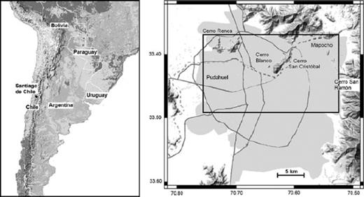
Location of Santiago de Chile (left-hand panel). Basin of Santiago (right-hand panel). Areas of high housing density are toned. Major highways are marked by dark grey lines. The dashed line is the Mapocho River. Locations mentioned in the text are indicated. The area of investigation is marked by the black rectangle.

Open in new tabDownload slide

The surface geology of Santiago de Chile can be divided into several types, as shown in Fig. 2. In the central and southern parts of the city, sediments consist of very dense coarse gravel with cobbles (Valenzuela 1978). In the northwestern part, recent alluvial deposits, consisting of silty soils, can be found, with a transition zone existing between these two areas. Stiff pumice of volcanic origin (i.e. pomacite) can be found in the western parts of the city (Pudahuel district). Artificial fill covers the riverside of the Mapocho River in the central part of the city. The spatial extension of each formation at depth is not well constrained.

Figure 2.

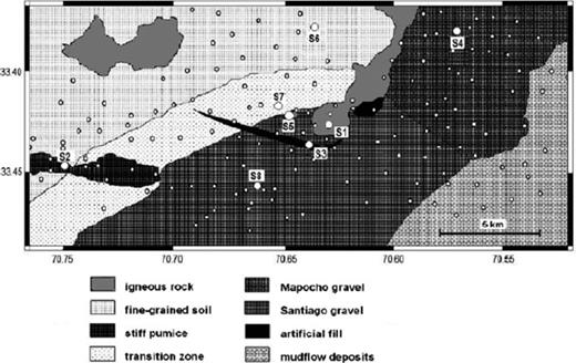
Simplified map of surface geology of the investigated area. Large spots indicate the locations of the installed seismic stations (see also Table 1). Small spots show sites where measurements of ambient seismic noise have been carried out.

Open in new tabDownload slide

The basement of the Santiago basin is believed to result from volcanic activity aged between the higher Oligocene to the lower Miocene. The bottom of the basin, known from gravimetric measurements (Araneda et al. 2000, Fig. 3), corresponds to an uneven surface that conceals some hill islands such as Cerro Santa Lucia and Cerro Renca. The alignment of some of these chains, such as that for San Cristobal, Chena and Lonquén, suggests that there might have been a structural control. The basin itself is covered with sediments, most of which have been transported from the Andes mountains by a branched river system. Some deposits are believed to result from volcanic mud flows or glaciers. The thickness of the sedimentary cover varies over short scales and can exceed more than 550 m. One must, however, keep in mind that the basin geometry, characterized by sharp lateral and vertical variations of the various units, is rather complex and would therefore have a strong influence on the frequency band affected by amplification.

Figure 3.

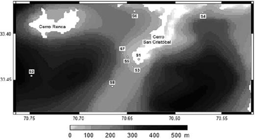
Thickness of the sedimentary cover of the investigated area as determined by interpolation of gravimetric data (Araneda et al. 2000). White areas can be identified as the hills Cerro Renca and Cerro San Cristóbal. Locations of the installed seismic stations are indicated.

Open in new tabDownload slide

3 Field Experiments

A network of eight seismological EarthData Logger PR6–24 instruments equipped with a Mark L-4C-3D sensor was deployed in the northern part of Santiago de Chile, covering the different geological units (Table 1, see also Fig. 2). We used sensors with a resonance frequency of 1 Hz, which were found to be suitable for investigation, especially when H/V peak results are expected to occur also down to 0.1–0.2 Hz (Strollo et al. 2008a,b). Installation of the network started on 2008 March 20, and the stations were removed after 2008 May 26, with exception of station S8, which had been removed some days before. A brief description of the soil conditions at the sites of the permanently installed stations based on borehole data and previous investigations compiled by Valenzuela (1978) and Araneda et al. (2000) is given below. Note that there is a degree of uncertainty in the depth of the bedrock due to interpolation and the inversion procedure of the gravimetry data between the measurement sites, which were spaced with an interstation distance of 500–1000 m.

Table 1.

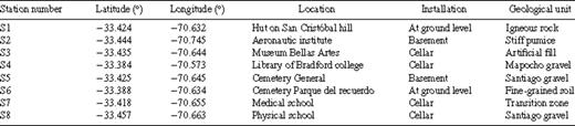
Network information.

Open in new tabDownload slide

Station S1: Igneous rock (outcropping San Cristóbal hill) composed of andesite and granodiorite. The San Cristóbal hill rises almost 300 m above the surrounding plain. The hut housing the instrument is approximately 30 m below the top of the hill. Since S1 is situated on rock, it can serve as a reference station, although topographic effects and perturbing influences cannot be excluded as discussed in the following.

Station S2: Pumacit deposits consisting of volcanic ash and pumice accompanied by fragments of rocks that are occasionally included in the overlaying the gravel layer. The thickness of the pomacite layer is around 45 m, with the depth to the bedrock being around 380 m.

Station S3: Heterogeneous materials ranging from sand to gravel rubble and waste. Poor quality of soil as a foundation, as there is no control regarding the composition and the degree of compaction. Depth to the bedrock is around 80 m.

Station S4: Alluvial deposits of the Mapocho river consisting of very dense gravel and unsaturated soil accompanied by sandy gravel, sand, silt and clays. Depth to the bedrock is around 90 m.

Station S5: Transition zone between Santiago gravel and fine grained soil including thick clay material layers. Large horizontal and vertical stratigraphic variations can be found within this zone. Gravimetric data suggest that the depth of the bedrock is around 185 m, but this might be questionable since the station is located close to an outcrop of the small Cerro Blanco. The thickness of the sedimentary cover decreases rapidly when approaching this outcrop, and less smooth bedrock topography is observed (Valenzuela 1978).

Station S6: Fine grained soil of Santiago's northwest of silt and inorganic clay with thin horizons of gravel and volcanic ash. Depth to the bedrock is around 136 m.

Station S7: Santiago gravel derived from alluvial from the river Mapocho and to a lesser part from the river Maipo. The soil is characterized by a large gravel compactness in a sand-clay matrix. Depth of the bedrock is around 177 m.

Station S8: Santiago gravel from the river Maipo alluvium and, to a lesser degree, from the river Mapocho. The soil is characterized by a large gravel compactness in conjunction with clay and a lesser amount of sand. Depth of the bedrock is around 95 m.

All permanent stations were installed inside buildings and were placed in their room's corner and, whenever possible, in cellars. All stations were synchronized using GPS reference time, however, station S8 lost its GPS signal some time after installation. Although this might effect the localization of earthquakes, there is obviously no influence on the spectral shapes. The signal was recorded at each site with a sampling rate of 100 samples s⁻¹. Due to the high level of noise within the urban area, which increases either the chances of false triggering or the risk of not triggering on the weak earthquakes, all stations were set to continuous recording. Therefore, in addition to the recorded earthquakes, a huge amount of ambient noise data was recorded.

Additionally, from May 19 to June 13 2008, noise measurements were carried out in the northern part of Santiago de Chile using the same setup described above. At each site, the signal was recorded for at least 25 minutes, leading to 146 measurements of ambient noise being carried out (measurement sites are shown in Fig. 2). For almost all the measurements, the sensor was placed directly on the ground (i.e. mown grass, not overgrown soil), with only few measurements carried out on asphalt. For all the measurements, the sensor was protected against wind. On some days, rain had been slight to moderate, but it has been shown (Chatelain et al. 2008) that rain has no notable influence.

4 Seismic Event Recordings: Data Aquisition and Analysis

4.1 Seismogram analysis

While the network was installed, 38 earthquakes with sufficient quality were recorded by at least four of the eight stations. Table 2 shows all the hypocentral parameters and magnitudes according to the PDE (Preliminary Determination of Earthquakes) catalogue. The list includes only earthquakes with an epicentral distance to the network of at least five times the maximum interstation distance, which is 17 km between stations S2 and S4, to exclude path effects for waves travelling to the stations. Altogether, 10 local, 22 regional and six teleseismic events are listed. As almost all earthquakes had been recorded by all stations, a detailed study can be accomplished; an exception is station S4, by which only 14 events with sufficient quality were recorded.

Table 2.

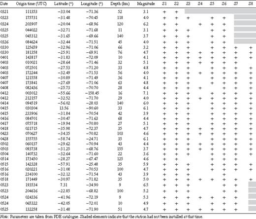
Events recorded by network between 2008 March 21 and May 26.

Open in new tabDownload slide

As an example, Fig. 4 shows the unfiltered recordings of the NS component for all stations of one local event. It can be seen that stations S2 and S6, which were located close to very busy roads, were affected by higher noise amplitudes whereas, for example, for stations S1, the reference station, and S5, the latter being located at a quiet part of a cemetery, the noise levels are much lower.

Figure 4.

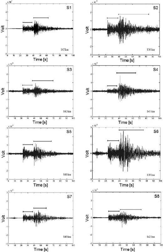
Comparison of NS recordings of a local earthquake on 2008 April 12, 21:21:57 UTC. Some stations show higher noise level due to the environment where they had been installed. The station ID and the hypocentral distances, as well as the time windows for P- and S-wave analyses are indicated.

Open in new tabDownload slide

4.2 Time domain analysis and earthquake duration

Quite different amplitudes and durations are observed at separate stations, despite their proximity. Although the amplitude ratio can differ by more than a factor of two compared with reference station S1 (see, e.g. station S6), Fig. 4 also shows clearly the lengthening of ground shaking for the basin sites. We calculate the duration of an event by ignoring the first and the last 5 per cent of the velocity square integral and considering the remaining 90 per cent as the significant contribution (Trifunac & Brady 1975). Several other definitions of earthquake durations can be found in a review by Bommer & Martínez-Pereira (1999).

The durations of all recorded events were divided by the corresponding duration recorded at the reference stations S1. Results of the mean duration ratios and standard deviations are shown in Table 3. As can be seen, the duration of ground shaking is increased, on average, by a factor of nearly 2, with a maximum of 2.27 at S6; only at station S5 the duration ratio is close to 1. This might be due to the location of the station close to (approximately 350 m) the outcrop of igneous bedrock at Cerro Blanco. Only a small sedimentary cover underlies S5, resulting in a lower amplification and ground motion duration. As already seen in Fig. 4, station S6 not only shows largest amplitudes but also most significant lengthening of the duration. Due to the large standard deviations that can be found in Table 3, we also performed a F test, which does not allow rejecting the null hypothesis of equal distribution at 95 per cent confidence level, meaning that there is a statistically significant correlation between the lengthening of duration for different stations.

Table 3.

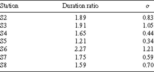
Duration ratios and standard deviations for stations located in the basin relative to the duration of the reference station S1.

Open in new tabDownload slide

In Fig. 5, the duration ratios calculated on the basis of both local, regional and teleseismic earthquakes for stations S5 and S6 with respect to those observed at station S1, as a function of backazimuth and magnitude are shown. A large scattering of duration lengthening in the middle of the basin is observed. However, the recorded earthquakes do not cover the entire backazimuth range and therefore do not allow us to assess if there is any clear dependence between the location of the event and the observed duration. On the other hand, a correlation between the extension of duration and the event's magnitude, rather than the epicentral distance, seems to exist: local events occurring with a lower magnitude (squares in Fig. 5b) show only a slight lengthening of the duration, whereas for regional and teleseismic events, a significant increase in duration is observed, which is an expected result. This might be explained by considering the different types of waves and the resulting incident angles arising from local, regional and teleseismic events. Hence, to investigate the increase in ground shaking and the spectral amplifications more thoroughly, a detailed analysis on the spectral ratios of the earthquake data has been performed.

Figure 5.

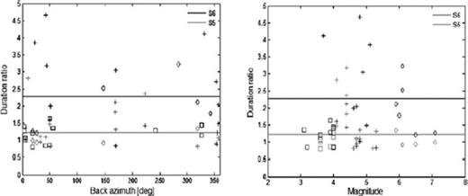
Duration ratios calculated for stations S5 and S6 with respect to the duration estimated at station S1. The ratios are shown against the angle of the backazimuth (left-hand panel) and magnitude of the event (right-hand panel). Squares, crosses and diamonds represent local, regional and teleseismic events, respectively. The horizontal lines correspond to the mean duration ratios for stations S5 (grey) and S6 (black).

Open in new tabDownload slide

4.3 Frequency domain analysis

To calculate the spectra for all the events, the recordings were first checked visually, and only those showing good signal-to-noise (S/N) ratio, allowing for detecting P- and S-wave arrival, were considered. Time windows for P- and S-wave analysis were then selected. The P-wave window starts 0.7 s before the P-wave arrival and ends before the S-wave arrival, when the P-wave energy reaches 90 per cent of its maximum. The same applies for the S-wave window. After correcting for instrumental response, each window was cosine tapered (5 per cent) and a Fast Fourier Transformation (FFT) for each seismometer component was performed. Spectral amplitudes were smoothed using the Konno & Ohmachi (1998) recording window (b = 40), ensuring smoothing of numerical instabilities while preserving the major features of the earthquake spectra that were considered valid only when the S/N ratio is greater than 3. The horizontal component spectra were calculated considering the root-mean square average of the N-S and E-W component spectra.

First, the EHV ratio was calculated for all events, separately for P- and S-wave windows (Fig. 6). It has been shown that EHV and SSR methods usually provide site responses with similar shapes when only the S-wave part of the seismogram is used; the P-wave part is found to provide consistent results only in some cases (see, e.g. Castro and the RESNOM working group 1998). Parolai et al. (2004b) found that EHV P and S waves show the same features, although the amplitude of EHV P waves is smaller. Therefore, we considered both parts separately. Additionally, the SSR method was applied to all recordings using S1 as a reference station, due to its location on igneous rock and its nearly flat response in the EHV spectrum. SSR curves for all stations are shown in Fig. 7. The shape of site responses between P and S waves is again quite similar.

Figure 6.

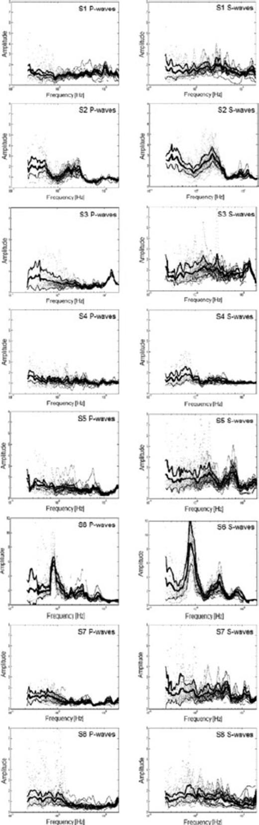
EHV calculated for P and S waves for all events with a signal-to-noise ratio larger than 3. Thick lines show medium ± one standard deviation. Please note the different amplitude scaling for station S6.

Open in new tabDownload slide

Figure 7.

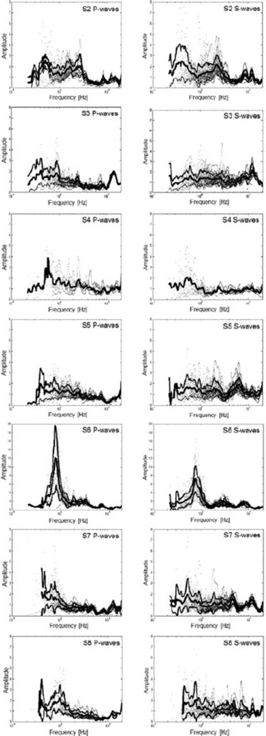
SSR calculated for P and S waves. Thick lines show medium ± one standard deviation. Please note the different amplitude scaling for station S6. For station S4, no standard deviation has been calculated due to too few recordings.

Open in new tabDownload slide

5 H/V Ratio of Ambient Noise: Data Aquisition and Analysis

As all the stations of the network were set to continuous recording, a huge amount of ambient seismic noise was recorded, allowing us to further investigate the long term stability of the NHV peaks and to verify the existence of differences in the results when using recordings from day and nighttime. The data also provided the means for comparing amplification factors obtained from the NHV peak with those determined by other methods.

For data processing, each noise recording was divided into 60-s-long windows tapered with a 5 per cent cosine function. As a rule of thumb, it is generally accepted (Parolai et al. 2001; Bard & SESAME WP02 team 2005) that the shortest window length has to be selected to include at least 10 cycles of the lowest frequency analysed. So, a window length of 60 s can be considered long enough to accomplish the analysis down to a frequency of at least 0.2 Hz. Instrumental correction and smoothening were carried out in analogy to earthquake data analysis. After checking visually for anomalies between Fourier spectra of the N-S and the E-W components, both spectra were then averaged (root-mean square), obtaining the horizontal component Fourier spectrum. Afterwards, we calculated the spectral ratios between the horizontal and vertical components, and finally, we determined the logarithmic mean of all the H/V ratios for a given site. For our studies, the number of selected windows (20–30) for this frequency range guarantees stable results, following Picozzi et al. (2005).

To estimate the stability of the peak in the NHV curve of the installed seismic stations, both in terms of frequency and amplitude, several curves were calculated using data recorded some time after the installation of the stations and before their removal with a time lag of 7 weeks. For both dates and all eight stations, NHV curves were calculated at midnight (04:00 UTC) and at noon (16:00 UTC) on the same day, respectively. Results are shown in Fig. 8. The analysis clearly shows that the shape of the NHV curves is not uniform, even though no large differences between recordings at midnight and at noon seem to occur.

Figure 8.

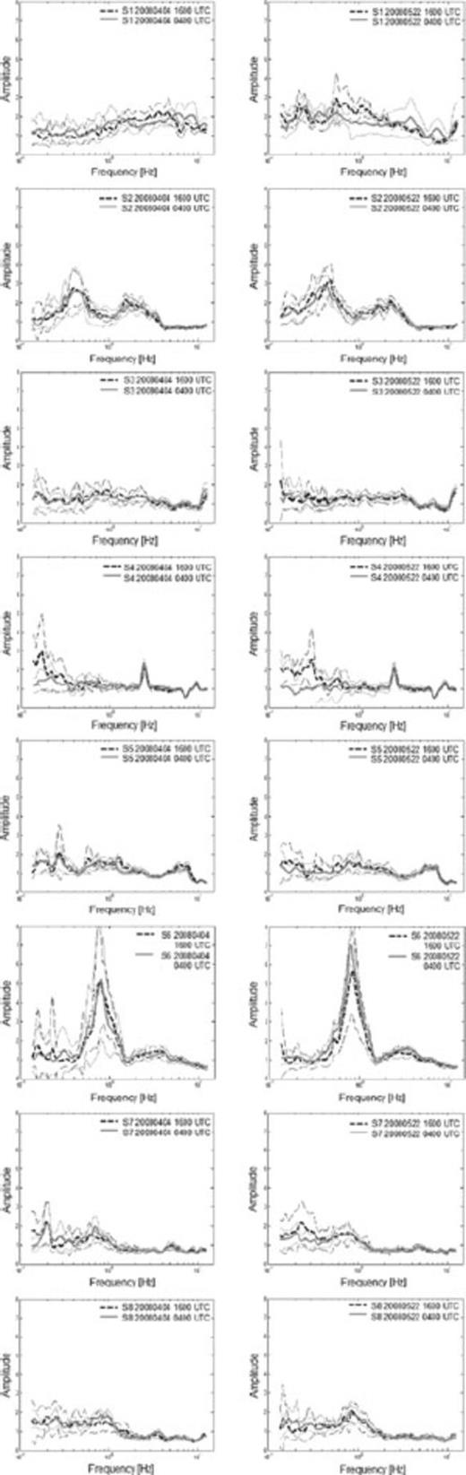
Average NHV ± one standard deviation calculated at noon (16:00 UTC) and at midnight (04:00 UTC) for the same day. Figures on the left-hand panel show recordings of 2008 April 4, figures on the right-hand panel recordings of 2008 May 22.

Open in new tabDownload slide

When comparing Figs 6 (EHV curves), 7 (SSR curves) and 8 (NHV curves), an all-embracing and detailed analysis is possible and is outlined below.

6 Results and Discussion

6.1 Seismic event and microtremor recordings: comparison of different techniques

6.1.1 S1 (reference station, no SSR curve)

As expected, no clear peak can be identified in the NHV curve, although the station shows little amplification over a broader frequency range (<5 Hz) in the NHV spectral ratios. To check if topographic effects are responsible for the small amplification, we investigated the directional variation of the NHV spectral ratio according to Del Gaudio et al. (2008). Therefore, we calculated an average NHV spectral ratio consisting of 20 NHV curves, selected randomly using recordings from day- and nighttime over the entire installation period. In Fig. 9 the mean NHV values are represented by a polar diagram. Although differences between the maximum and minimum amplitude at the same frequency are small a clear preferential direction in the azimuthal distribution of the amplitude is shown: the relative maximum is oriented along N70°E, the maximum slope direction, confirming the results found by Del Gaudio et al. (2008). It has to be mentioned that significant topographic slopes are found at all outcrops of the igneous rock.

Figure 9.

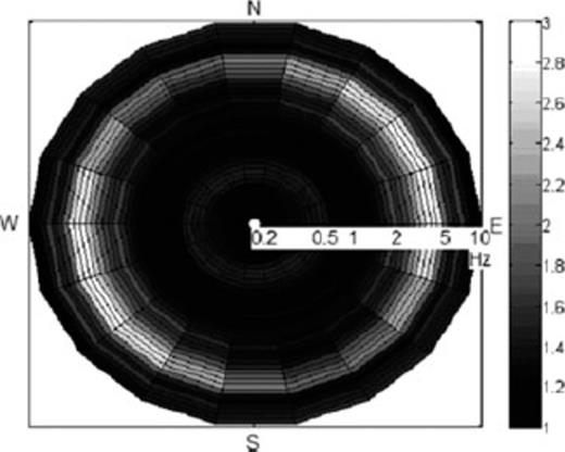
Polar diagram of mean NHV spectral ratio for station S1 calculated at 20° azimuth intervals for an average of 20 randomly selected NHV measurements.

Open in new tabDownload slide

For the NHV curves recorded on 2008 May 22, there are small differences between the recordings at noon and at midnight. Due to limited sites on the San Cristóbal hill providing a power supply, the installation of the station was not far away from the mountain station of the funicular onto the San Cristóbal hill. As this area is frequented by people during daytime, the difference might be explained by these disturbances.

When looking at the earthquake data, the EHV curve of the S waves shows a slightly higher level of amplification with respect to both the P-wave windows and the NHV curve. Although only a slight influence of the topography on the amplification for NHV spectral ratios at S1 is found, this trend cannot be seen when considering EHV spectral ratios—no azimuthal distribution is found, or it might be masked by the large scattering of the earthquake data. This might indicate that it is justified to choose this station as a reference.

6.1.2 S2

Although all the NHV, EHV and SSR curves show a consistent shape, the amplification of the S-wave windows is generally slightly larger compared with the P-wave windows. Whereas the second peak around 2 Hz is smaller than the first one at 0.45 Hz, in the NHV curve, both peaks are of the same amplitude for EHV and SSR. The secondary peak at around 2 Hz can be explained by considering local geological conditions—as described above, at this site a layer of pomacit is overlaying gravel, therefore a second impedance contrast might reasonably explain this peak. The frequencies at which the peaks occur seem to be at first-order consistent with the thickness of the sediments obtained by the gravimetric data set. Additionally, some events show (quite small) peaks in the EHV and SSR curves around 8.7 and 13 Hz, which the NHV method is unable to detect. These peaks might be related to relative superficial impedance contrasts, which is also supported by Bravo (1992). No differences between the recordings made at day- and nighttime are visible in the NHV curves.

6.1.3 S3

Although there is a strong scattering, no striking significant peak can be seen in the noise or in the earthquake curves. Several small peaks for some events appear in the EHV curves. In general, the amplitude of the S-wave window curve is, in this case also, slightly larger than the one of the P waves.

6.1.4 S4

Although the P-wave curve of the EHV remains flat, the S-wave curves of EHV and SSR show some slight amplification in the frequency range between 0.5 and 0.9 Hz. Due to the few recorded earthquakes with good S/N ratios, no statements can definitively be made about the P-wave windows of the SSR results. On the other hand, although the NHV curves seem to be flat, a clear peak at exactly 2.5 Hz and a small one at 9.3 Hz are visible in all NHV curves. When calculating the spectra for each component separately (see Fig. 10), obvious differences occur. In fact, the peak at 2.5 Hz is not found in the (N-S)/V component of noise whereas it clearly appears in the (E-W)/V component, with the opposite situation for the small peak at 9.3 Hz. The standard deviations for all curves remain quite small. As it is really unlikely to have two sources oriented at exactly 90° from each other without any influence on the orthogonal component, and since it has already been reported (e.g. Gallipoli et al. 2004b; Cornou et al. 2004) that noise, and even earthquake, recordings are strongly influenced by the proximity of structures, we believe that these frequencies might be related to the first two translational modes of the building in which the sensor was located. Furthermore, the fact that these peaks are not related to the soil response is also supported by the results of the single-stations NHV measurements determining much lower frequencies for this area (see Section 6.4 and Fig. 13).

Figure 10.

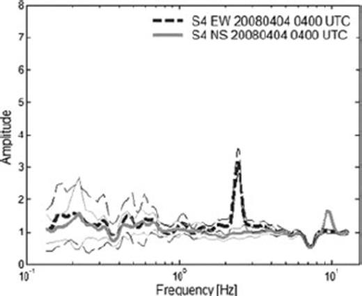
EW/V and NS/V spectra ± one standard deviation for the recording on 2008 April 4 of station S4.

Open in new tabDownload slide

Figure 13.

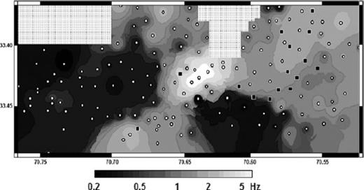
Map of the fundamental resonance frequency of the investigated area. Spots indicate sites where measurements of ambient seismic noise were carried out. Black squares indicate flat NHV recordings: these values have not been considered for mapping the fundamental frequency. In the hatched area, no measurements were carried out, hence results are only due to interpolation and therefore masked.

Open in new tabDownload slide

This example clearly confirms that all components of the Fourier spectra have to be checked carefully, and affects of the structure where the sensor is installed have to be accounted before analysing the results, to avoid misinterpretation.

6.1.5 S5

Although the curves have similar trends, the amplification retrieved by the S-wave window curves are higher than those of the P-wave windows, showing a peak at 6 Hz, which is only foreshadowed in the NHV curve and can hardly be seen in the P-wave curves. Over a broad frequency band between 0.5 and 3 Hz, all curves show slight amplification with amplitudes marginally below 2.

6.1.6 S6

All curves show a clear peak at 0.9 Hz, with amplitudes ranging between 5 (NHV curve) and 12 (SSR P waves). The peak of the fundamental resonance frequency is as a first approximation consistent with the thickness of the sedimentary cover provided by an interpretation of the gravimetry data. Peaks of higher harmonics at around 3 and 8 Hz can also be observed in the earthquake data, especially on the S-wave window curves, whereas the NHV curve show only small bumps over that frequency range.

6.1.7 S7

Due to a low S/N ratio, no reliable SSR curve below 0.4 Hz could be determined. All curves remain quite flat. Nonetheless, when checking the EHV and SSR S-wave curves, a few events show amplification at 4.8 and 13 Hz, respectively, but the amplitudes remain rather small. This trend is not visible for both P-wave curves. As the translational modes of the building are excited much better by S waves than by P waves (e.g. Wegner et al. 2005), and as the major axes of the building almost coincide with the N-S and E-W direction, both small peaks might again be related to the first two translational modes of the building. In the NHV curves, no clear peaks can be found, although there are slight elevations for frequencies around 0.2 and 0.7 Hz. Considering the thickness of the sediments obtained by gravitmetry data, the fundamental frequency is expected to occur around 0.7 Hz, that is, the first peak is not the fundamental one. In addition, the small amplitude of the peaks might indicate a low impedance contrast.

6.1.8 S8

Due to a low S/N ratio, no reliable SSR curve below 0.4 Hz could be determined. Large scattering appears with some events showing amplification around 1 Hz, which might also be supported by a bump in the NHV curve recorded on May 22, whereas this bump cannot easily be seen in the curves of April 4. The thickness of the sedimentary cover also suggests amplification at around 1 Hz.

6.2 Summary

Generally, there is a good agreement in the shape and the location of the fundamental resonance frequency as found from the SSR, EHV and NHV curves. EHV and SSR spectral ratios show similar shape and amplitude because the small amplification found at station S1 due to topographic effects does not influence the results. As only events with an epicentral distance of five times the maximum interstation distance have been considered for analysis, the SSR technique is found to provide a more reliable estimate of the site response because effects due to the path and the radiation of the source are minimized, respectively.

In general, the level of amplification is surprisingly low at several stations located within the basin (i.e. S4, S5 and S8). Reliable EHV and SSR site responses, in general, can only be obtained when earthquakes are distributed all around the stations at different distances. Due to the tectonic situation, the recorded earthquakes are mainly clustered in two narrow azimuthal ranges, as can be seen in Fig. 5(a), but no influence is believed to arise from this shortcoming due to the relatively large number of events used. To definitively exclude any influence of the clustering of the recorded events and to obtain a clearer view of earthquake location dependencies, further work is needed. The main reason for the small amplitude at several sites is therefore believed to result from a low impedance contrast, a conclusion supported when considering the soil conditions below the sites (see site characterization above) and also by the findings of Bravo (1992).

Differences between NHV and earthquake spectral ratios can be found in terms of the amplification level—most of the earthquake data show a higher level of amplification than NHV curves for large ranges of the frequency band. This is also strengthened by Fig. 11, where the ratio of SSR divided by NHV for all stations in the frequency range 0.2–20 Hz (0.4–20 Hz for S7 and S8) is shown. NHV seems to give a lower amplification, especially for lower and higher frequencies, whereas for frequencies around 1 Hz, the ratio between SSR and NHV takes a value below one. Some stations (e.g. S2 and S6), located on thick sediments, have clear peaks related to higher harmonics in the EHV and SSR curves, with amplifications sometimes exceeding 3. Because NHV is generally expected to estimate only the fundamental resonance frequency (or to provide amplifications over a narrow frequency band around it), it could be expected to underestimate more significantly the level of amplification at frequencies higher than the fundamental one. Therefore, the ratio between SSR and NHV is expected to be frequency-dependent and to differ between analysed stations, depending on the position of the peak relevant to the fundamental frequency.

Figure 11.

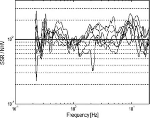
Ratio between standard spectral ratio and H/V site responses from seismic noise.

Open in new tabDownload slide

Additionally, when comparing spectral ratios of P- and S-wave windows, both spectra share similar features as long as the frequencies of maximum amplification are considered (if appearing in the P-wave curve), but amplitudes in the P-wave curves are often considerably lower. However, this difference might be explained by the hypothesis that the P-wave window results are mainly related to converted waves. Since there exists a low impedance contrast, the amount of conversion is limited, and the S/N ratio in the windows is low (see Fig. 4).

Finally, in Fig. 8, it can be seen that the shape of all NHV curves is quite stable, which means that if there are any peaks, they occur at almost the same frequencies and show the same amplitudes. Also, no differences between recordings during day- or nighttime are observed, with the exception of station S1 on 2008 May 22, as discussed above. Since transient noise is expected to be generated mainly by nearby sources and generally affects noise spectra at frequencies higher than 1–2 Hz (e.g. McNamara 2004), this might confirm that transients have no (or only a little) influence on the NHV ratio, a result already shown by several studies (e.g. Mucciarelli et al. 2003; Parolai & Galiana-Merino 2006).

We can therefore conclude that no notable NHV variation with time has been observed. This result can be used for further experiments by analysing noise measurements within the city, as the amplitude and the fundamental frequency of the NHV peak is not influenced by the time of measurement and the environmental conditions.

6.3 Single station NHV measurements

As mentioned, in addition to the earthquake recordings, measurements of seismic noise were carried out at 146 different sites in the northern part of Santiago de Chile. There exist several criteria how to qualify the reliability of a peak, including its absolute amplitude, the relative amplitude value with respect to other peaks and by considering the standard deviation. We used the following guidelines proposed by the SESAME consortium (see Bard & SESAME WP02 team 2005 for further details):

• (1)

  The maximum peak amplitude of the NHV curve is higher than 2.

• (2)

  There is a lower threshold frequency f⁻ in the frequency range fǀ_H/V/4 < f⁻ < fǀ_H/V such that the amplitude ratio is fulfilling (Therein, fǀ_H/V indicates the fundamental frequency and Aǀ_H/V the amplitude at that frequency).

• (3)

  There is an upper threshold frequency f⁺ in the frequency range fǀ_H/V < f⁺ <4 fǀ_H/V such that the amplitude ratio is fulfilling .

• (4)

  The standard deviation has to be lower than a frequency-dependent threshold.

To be sure that the site is likely to experience ground motion amplification, at least three of these four criteria should be achieved; then the peak frequency can be considered as a reliable estimate of the fundamental frequency of the site.

All average NHV curves were systematically analysed following the SESAME recommendations. In the end, 115 reliable NHV curves fulfilled these criteria. In another 16 curves, a clear peak was visible although not fulfilling at least three of the four criteria mentioned above, whereas for 15 curves, no reliable peak could be determined. Hence, these 15 latter curves were not considered for further analysis. In Fig. 12, examples of the different kinds of curves are shown.

Figure 12.

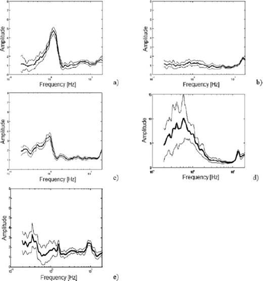
Examples for different NHV spectral ratios ± one standard deviation. Please note the different amplitude scaling for panel d. See text for further discussion.

Open in new tabDownload slide

When the NHV peak is clear (Fig. 12a), a large impedance (i.e. velocity) contrast between the sedimentary cover and the bedrock is expected to exist, hence it is very likely that ground motion is amplified at this site. Flat NHV curves (Fig. 12b) and peaks with a low amplitude are located at the surface of dense sediment locations, that is, mainly gravel. A low impedance contrast resulting from stiff sediments underlain by bedrock is likely to exist, and therefore one might expect rather small amplification. Although flat NHV curves within a much wider area in the Santiago basin were found by Bonnefoy-Claudet et al. (2009), these authors suggest that NHV curves showing no peak are from stiff sediment sites. Curves like those in Fig. 12c show quite broad peaks spread over the entire basin, with no correlation with topographic characteristics and local geology. The influence of wind can be excluded as the sensor and cables were protected, and no measurements were made in the immediate vicinity of trees or buildings. On the other hand, gravimetric data (Araneda et al. 2000) and cross-sections (Pasten 2007) show that at some sites, the thickness of the sedimentary cover varies over short distances. Previous studies (Wooleroy & Street 2002) show that broad NHV peaks can be obtained at sites with a complicated subsurface geometry and large near-surface shear-wave velocity contrasts. Although there might sometimes be difficulties in determining an exact fundamental frequency, at least a bound can be identified, where one can be confident that amplification will occur. Large standard deviations like those shown in Fig. 12(d) often mean that ambient vibrations are strongly non-stationary and undergo some kind of perturbations that might be removed by a longer recording duration. Nonetheless, as shown here, a clear peak is visible which can be used for determining the fundamental resonance frequency of the site. Finally, curves, such as shown in Fig. 12e, would actually have to be discarded, as they do not fulfill at least three of the four standard criteria—here a too marginal decrease for low frequencies and a large standard deviation. Nonetheless, three clear peaks at around 0.35, 1.7 and 10 Hz are visible. As the recording presented in Fig. 12e was only 900 m away from the site where station S2 had been installed, and also, the shapes of Fig. 12(e) and the EHV and NHV curves of S2 (Figs 6 and 8) look quite similar, the peaks can be considered to be reliable due to their spatial coherency.

Altogether, although 31 curves do not always fulfill all the standard conditions for a reliable curve as mentioned above, 16 of these were used for further analysis because a peak was clearly visible and the criteria hereunto seemed to be too restrictive. Most of these measurements were carried out at sites with a low impedance contrast in the eastern part of the investigated area, which means that the peak amplitude is often slightly below 2, and the decrease (predominantly towards lower frequencies) is too small, whereas neighbouring sites fulfilled the criteria showing peak amplitudes beyond 2. Usually, the foremost measurements would have to be discarded, but their reliability (similar to the example of Fig. 12e) was assessed by considering spatial coherency and geological and geophysical data sets. Hence, due to the experimental character of the NHV method, visual inspection of the data should always be performed.

6.4 Fundamental resonance frequency map of the investigated area

The analysis of the fundamental resonance frequencies calculated for all sites allowed us to draw a map of the fundamental frequencies of the investigated area (Fig. 13). In general, the frequency varies slightly in space without large differences between neighbouring sites. Sites showing a flat NHV curve are predominantly located in the eastern part of the investigated area and are almost all located on gravel, consistent with Bonnefoy-Claudet et al. (2009). These units are characterized by stiff sediments with a rather high S-wave velocity (Bravo 1992). Hence, no sharp velocity contrast may exist at depth at such sites. On the other hand, there are also several NHV curves located on gravel, showing a peak slightly higher than two fulfilling the standard criteria.

Fig. 13 clearly shows that the entire area is characterized by relatively low frequencies below 1 Hz. Only when one considers sites close to the city centre and around the San Cristóbal hill, the fundamental frequency does increase more rapidly. In this part of the basin, the thickness of the sedimentary cover is decreasing and the bedrock outcrops, as evident by the San Cristóbal hill (see Fig. 3). There is also a rapid decrease in the sediment thickness toward the northwest of the investigated area, but no increase in the fundamental frequency can be observed there because no noise measurements have been carried out in the immediate vicinity of the Renca hill. Only two nearby sites show a trend toward higher frequencies.

On the other hand, frequencies below 0.5 Hz can be found in the west and toward the south-southeast of the investigated area. The sedimentary cover thickness reaches more than 500 m in these parts of the basin, supporting the general trend of the fundamental frequency decreasing with increasing sedimentary cover thickness.

Considering that, as a first approximation for Chilian structures, the relationship between the height of a building and its fundamental period of vibration T can be expressed by

1

where 50 m s⁻¹ ≤ C ≤ 60 m s⁻¹ (Guendelman 2000), we expect that for most parts of the city the natural frequency of the soil will match the frequency of buildings with more than 10 storeys. However, during the 1985 Valparaiso earthquake, there was considerable damage to small-sized adobe structures, whereas the high-rise structures up to 20 storeys performed quite well, with only minor damage to finishes and non-structural features (Astroza et al. 1993). In the areas of highest intensities, the comparison between the NHV peak frequencies and damage to houses of a few (≤ 4) stories reveals that where NHV peak frequencies do not exceed 3–4 Hz, more damage was observed on those houses having a natural frequency above 5 Hz. A recent study (Gallipoli et al. 2008) confirms, as reported by many previous authors, that theoretical height-period relationships like eq. (1) often overestimate the experimental data in terms of building periods, by taking into account the structural system only without any specifications regarding the system characteristics like the flexibility of the foundation or the stiffness of the infills. However, one must remember that the NHV method provides only a lower border of the amplification level and of the frequency, as stated already by Lebrun et al. (2001). On the other hand, as there is also rapid rebuilding of the city, with the replacing of old structures by tall multistorey buildings, especially in a great circle around the city centre, the frequency of the soil cover could be close to their fundamental frequency of vibration. Moreover, higher harmonics also might correspond to the eigenfrequency of these buildings or even to higher harmonics of the buildings.

7 Conclusions

The investigation carried out in this work showed that site effects have a considerable influence on earthquake ground motion in the basin of Santiago de Chile. This observation is consistent with the relatively variable damage distribution observed following the 1985 Valparaiso earthquake.

For the first time, eight seismic stations were installed in the city of Santiago for recording earthquake signals. 38 events at different distances have been recorded with sufficient quality by the network. Time domain analysis shows differences in amplitude and lengthening with respect to a nearby rock site, up to a factor of more than two. In the frequency domain, we applied three different techniques for estimating site effects at the seismic stations. The comparison of the NHV ratio with EHV and SSR results illustrated a generally good agreement in the shape of all three curves, especially for the peak of the fundamental resonance frequency. Significant amplification (i.e. amplitudes exceeding 2 for the fundamental frequency) does not depend on the thickness of the sedimentary cover, but only on local geological conditions that can vary rapidly (see e.g. Pasten 2007). Higher harmonics, which may overlap with the resonance frequencies of neighbouring buildings, are often not visible in the NHV spectra but may not necessarily be damped out under such conditions. Therefore, NHV spectra might only serve as the lower frequency bound for site amplifications. Nonetheless, at some stations, the amplitudes are quite small, which might be related to low impedance contrasts and the damping of seismic waves. Additionally, the results obtained using P-wave windows often share similar features with those for S-wave windows because the frequencies of maximum amplification are almost the same but have significantly lower amplitudes. We also show that the NHV spectral ratios are quite stable with almost no dependence on the time and environment of the recordings.

Additionally, 146 measurements of seismic noise were carried out, analysing the recorded data according to the SESAME criteria (Bard & SESAME WP02 team 2005). If a clear NHV peak appears, a confident estimate of the fundamental resonance frequency is possible, but we also show that for a case like Santiago de Chile, NHV curves not fulfilling the strict criteria may also provide the soil resonance frequency or, at least, the frequency bands prone to amplification, especially when additional information on the geology is available. These results suggest that the quality criteria might sometimes be too restrictive. A similar conclusion was also reached by Bonnefoy-Claudet et al. (2009). On the other hand, the results show the importance of combining noise measurements with recordings of seismic events at characteristic sites. However, further work is necessary to clearify this debate.

The analysis of NHV spectral ratios enabled us to map the fundamental resonance frequency of the investigated area. We showed that peaks mainly occur at low frequencies below 1–2 Hz, but slight amplification also affects frequencies from 2–13 Hz. A general trend in the variation in the frequency range of amplification and the thickness of the sedimentary cover can be seen. However, differences can be explained by considering local variations in the sedimentary cover.

During the next phase of this work, we will establish a detailed model of the investigated area of the basin of Santiago de Chile by using the recorded ambient noise measurements and additional geotechnical and geophysical information. This data set might then serve as a basis for the realistic modelling of seismic wave propagation in the basin and therefore from this basis for hazard scenarios.

Acknowledgments

This work was supported by the Helmholtz research initiative ‘Risk Habitat Megacity’. We thank David Solans, Natalia Silva and José Gonzalez for installing and operating the seismic network and the field experiments. The comments of an anonymous reviewer and of Marco Mucciarelli, who pointed out the importance of considering the building structure for the data analysis, improved the manuscript. Matteo Picozzi and Angelo Strollo provided useful suggestions. The Geophysical Instrumental Pool Potsdam provided the instruments. Kevin Fleming kindly revised our English.

References