


Summary
We examine micro-earthquake records from a dense temporary array of ocean bottom seismometers (OBS) and hydrophones that has been installed from September to November 2005 at the trench outer rise offshore Nicaragua. Approximately 1.5 locatable earthquakes per day within the array of 110 × 120 km show the high seismic activity in this region. Seismicity is restricted to the upper ∼15 km of the mantle and hence where temperatures reach 350–400 °C, which is smaller than values observed for large mantle intraplate events (650 °C). Determination of moment tensor solutions suggest a change of the stress region from tensional in the upper layers of the oceanic plate to compressional beneath. The neutral plane between both regimes is located at ∼6–9 km beneath Moho and thus very shallow. Fluids, which are thought to travel through the tensional fault system into the upper mantle, may not be able to penetrate any deeper.
The earthquake catalogue, which seems to be complete for magnitudes above Mw = 1.6–1.8, suggests a strong change of the lithospheric rheology when approaching the trench. And b-factors, that is the ratio between small and large earthquakes increase significantly in the closest 20 km to the trench axis, implying that the crust and upper mantle is massively weakened and hence ruptures more frequently but under less release of stress. We explain this with a partly serpentinized upper mantle.
1 Introduction
In subduction zones most of the worldwide seismicity is released. The largest events are megathrust earthquakes occurring in the coupling zone between the overriding and the subducting plate. Seaward of the trench, however, bending of the incoming plate causes widespread normal faulting and seismic activity (Chappel & Forsyth 1979; Grevemeyer et al. 2007; Tilmann et al. 2008). Bending of the plate leads to a tensional regime on top of the oceanic plate grading into a compressional one beneath, both separated by a neutral plane (Chappel & Forsyth 1979). However, the energy released by large outer rise events, like the 1933 Sanriku Ms = 8.3 event, suggest that fracturing took place over the entire thickness of the lithosphere, thereby precluding the possibility that such events merely represent a surface tensile crack due to the flexure of the downgoing plate (Kanamori 1971). Such large scale lithospheric faulting is presumably due to a gravitational pull exerted by the cold sinking lithosphere (Kanamori 1971). Moreover, outer rise earthquakes are often related to seismic coupling in the megathrust fault (e.g. Christensen & Ruff 1988; Ammon et al. 2008). Thus, stress distribution in the oceanic lithosphere entering the deep sea trench is a superposition of bending forces, gravitational pull of the cold sinking slab, and coupling with the overriding continental plate (Christensen & Ruff 1988). Stresses acting in the trench-outer rise and hence the location of the neutral separating the tensional and compressional regime vary therefore spatially and temporarily during the seismic cycle (e.g. Taylor et al. 1996; Ammon et al. 2008). Intraplate normal faulting earthquakes in the tensional regime have been inferred to cut deep enough into the lithosphere to provide pathways for sea water to penetrate into the mantle (Ranero et al. 2003; Ranero & Sallares 2004; Grevemeyer et al. 2007), thereby altering peridotites into serpentinites (Ranero et al. 2003; Peacock 2001, 2003) that contain up to 13 weight per cent of water. Dehydration at greater depth may trigger intermediate-depth earthquakes (Meade & Jeanloz 1991; Kirby et al. 1996) and influence the melting under volcano arcs (Rüpke et al. 2002), though a largely unconstrained portion of subducted fluids may enter the deep Earth's interior, establishing a connection between the oceans and the Earth's deep water cycle (Rüpke et al. 2004).
Despite of its importance for subduction zone processes, little is known about the amount of serpentinite residing in the oceanic mantle and its maximum depth of occurrence as well as mechanisms controlling serpentinization in the trench-outer rise. We suggest that an important factor governing water percolation into the mantle might be the depth of the neutral plane, since it cannot be assumed that a compressional regime at greater depth supports water infiltration.
Most seismological studies on the stress regime of the oceanic lithosphere in the trench-outer rise are based on teleseismic and regional data (e.g. Christensen & Ruff 1988; Lefeldt & Grevemeyer 2008; Ammon et al. 2008). However, it is in general difficult to determine accurately hypocentre depth for shallow earthquakes occurring in the vicinity of deep sea trenches (e.g. Yoshida et al. 1992). Thus, estimations for the depth of the neutral plane and hence the cutting depth of normal faults may suffer from large errors.
In this study we present results from a local earthquake monitoring network, which was installed at the Outer Rise offshore Nicaragua. During a period of 2 month numerous local events have been observed within the network. Local earthquake data have been used to study earthquake distribution, spatial distribution of moment release, and the stress field derived from focal mechanisms to study processes changing the physical state and chemical composition of the subducting plate.
2 Tectonical Framework and Setting
The study area is located offshore Nicaragua and seawards of the Middle American Trench. Here, the oceanic Cocos Plate is subducted beneath the Caribbean Plate, whereat the Benioff zone can be tracked down to 220 km and shows a dip of 25° at the beginning of the seismogenic zone to 84° where the deepest earthquakes can be observed (Burbach et al. 1984; Protti et al. 1994).
High resolution multibeam bathymetry shows that bending-related faulting is pervasive across most of the ocean trench slope (Fig. 1). Some faults are tracked in the bathymetry for at least 50 km and multichannel seismic reflection data suggest that they cut more than 20 km into the mantle (Ranero et al. 2003).
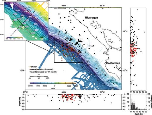
ORN and observed seismicity over a 2-month period. The events have been located using the HYP code and a preliminary velocity model (see Table S1 in supporting information). Red dots denote events that have been used for the calculation of the P-wave minimum 1-D model, meanwhile events presented by a black dot were excluded from the calculation for quality reasons. The depth always denotes depth beneath seafloor. All stations have been set to a depth of 0 km, to keep the calculation simple. The histogram in the lower-right corner gives a count of earthquakes per 1 km-interval. The total number of events for the depth interval 0–1 km is 56. Multibeam bathymetry from Ranero et al. (2003).
The idea that sea water might infiltrate through these faults into the lithosphere is perhaps supported by geochemical data from the volcanic arc that suggests that mafic magmas in Nicaragua have water concentrations among the highest in the world (Roggensack et al. 1997). Furthermore, regional P-waves from intraslap events in 100–150 km depths show high-frequency late arrivals, which could be caused by a 2.5–6 km thick low-velocity layer in the incoming plate (Abers et al. 2003). Such velocity anomalies at greater depth and pressure can be best explained by >5 weight percent of water in the subducted crust, giving a hydration degree 2–3 higher than inferred for other slabs. Thus, existing data suggests that the Nicaraguan slab may contain an unusually high amount of water.
3 The Outer Rise Local Earthquake Monitoring Network
The Outer Rise Network (ORN) was deployed during the RV Meteor M66/3 cruise in September 2005 and recovered 58 to 61 days later. In total 21 instruments provided data, among them 10 ocean bottom seismometers (OBS), each equipped with both a hydrophone and a three-component seismometer, and 11 ocean bottom hydrophones (OBH). Seismic wavefield was sampled at 100 Hz or 125 Hz. Spacing between instruments was 15–25 km, covering an area of 120 km × 110 km (Fig. 1).
3.1 Seismic data processing
To identify earthquakes in the continuous data stream an automatic trigger routine has been applied, considering only events that have been simultaneously observed on at least four stations within a 3-min time window. A total number of 1911 events were detected. Any further processing of the data was done manually.
For 297 events a preliminary location could be found (Fig. 1) using the linear earthquake location program HYP from the SEISAN earthquake analysis software package (Havskov & Ottemöller 1999) and a preliminary 1-D velocity model (see Table S1 in the supporting information, Appendix S1) based on seismic refraction data (Ivandic 2008; Ivandic et al. 2008).
4 Analysis
4.1 Hypocenter location and minimum one-dimensional velocity model
In most earthquake localization routines the velocity parameters must be known a priori, for example from active seismic tomography. Then, the observed travel times are minimized by changing the hypocenters, which represent the only free parameters, whereas the velocity model is kept constant. However, the travel time of a seismic wave depends on both, the seismic velocities sampled along the ray paths and the hypocenter parameters (Husen et al. 1999). Keeping one of these sets of variables fixed will most likely introduce systematic errors (Thurber 1992; Eberhart-Phillips & Michael 1993). Generally speaking, the calculation of hypocentres from travel time data is a non-linear problem, with the velocity model and the hypocenters as variables and is called the coupled hypocentre-velocity model problem (Crosson 1976;a Kissling 1988; Thurber 1992). Thus, an accurate hypocenter calculation requires the simultaneous inversion for the hypocenters and the velocity structure.
4.1.1 P-wave minimum one-dimensional velocity model
A minimum 1-D velocity model was obtained by using the software routine VELEST ( 1994, 1995), which allows the calculation of both the velocity model that minimizes the average rms values of all events and refined hypocenter parameters, in an iterative inversion procedure.
Events that were recorded at less than eight stations or had an azimuthal gap of >220° were excluded from the data set, which leaves a total number of 68 events, with 722 P-wave observations and 197 S-wave observations.
VELEST allows for station elevation, which is of advantage for most applications, since it implies that each ray is traced to the absolute position of each station. The shallowest station in the ORN was at 2820 m below sea level whereas the deepest one was at 5296 m below sea level, which gives a station-topography of approximately 2.5 km. The current version of VELEST requires that all stations are located in the first layer, resulting into a top layer of 2.5 km thickness with a constant velocity. This is rather unrealistic since the study area is characterized by a thin sediment layer of about 380 m thickness (Kimura et al. 1997), with a very low average velocity of 1570 m s−1 in the upper 180 m (hemipelagic sediment) and additional a thin crust (Grevemeyer et al. 2007; Ivandic et al. 2008) of 5.5–6 km with seismic P-wave velocities increasing with depth from 4.2 to 6.7 km s−1. Further, the strong velocity gradient in the sediments and upper crust would most likely introduce systematic errors and cause numerical instabilities if a thick top layer is used ( 1999). In addition, seismic refraction data (Grevemeyer et al. 2007; Ivandic et al. 2008; Ivandic 2008) suggest that the basic structure (thickness of sediments, depth of Moho, etc.) is roughly the same beneath all stations. Thus, it seems to be much more appropriate to neglect station elevations.
The first step of the inversion process is to find an appropriate layering for the P-wave inversion. Therefore, different layer thicknesses are tested with a wide range of realistic and unrealistic initial velocity models. After the inversion, the final model should have the same values independently from the initial model. In cases where instabilities observed, the model has to be refined.
Fig. 2 shows a layer test for a thick first layer and allowance of station elevations. A wide range of initial models leads to a wide range of final models, which suggests that a refined upper layer thickness should be used to achieve a better convergence. However, since all stations need to be located in the first layer, a thin upper layer is only possible if station elevations are neglected, which should rather influence the station correction terms than the velocity structure (Husen et al. 1999).
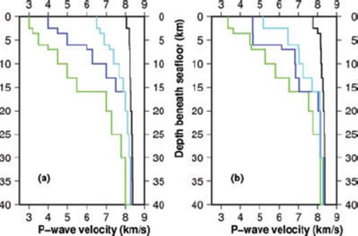
(a) Initial P-wave velocity model and (b) results after inversion with a thick first layer and with station elevations. Lines of the same colour in (a) and (b) always give a pair of starting and resulting model. The convergence is not satisfying due to the large thickness of the top layer.
The result of a layer test with a refined upper layer thickness and a neglect of station topography is shown in Fig. 3. Various initial models (Fig. 3a) all show convergence below 7 km beneath seafloor (Fig. 3b). Above convergence is not well-constrained.
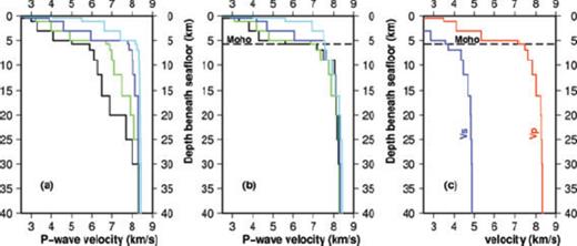
(a) Initial P-wave velocity model and (b) results after inversion with a refined upper layering and neglect of station elevations and finally used minimum P-wave 1-D velocity model (red line). Convergence is given below 7 km; in the upper layers only the velocity gradient can be resolved and not absolute values. (c) Final P- and S-wave 1-D model.
Most likely this is a result of both, the neglect of station elevations and the strong decrease of crustal velocities toward the trench (Ivandic et al. 2008). Since crustal velocities in this area are known from seismic wide-angle and refraction data, a combination of average velocities from active seismic tomography for the crust and of the 1-D velocity model for the mantle provides a very reliable velocity structure.
P-wave station correction terms are calculated during every iteration with VELEST and are applied for the subsequent iteration to account for geological subsurface structure and the neglect of station elevations (Husen et al. 1999). Final station corrections are shown in Fig. 4. Negative station corrections refer to an early arrival compared to the reference station, meanwhile positive values imply a late arrival. The final P-wave 1-D velocity model (Fig. 3) was obtained after 9 iterations with VELEST. The final all-over rms is 205 ms, which is acceptable low. The initial model consists of average velocity values from active seismic for the crust (see Table S1 in the supporting information, layer 2–6) and assumed values for the mantle.
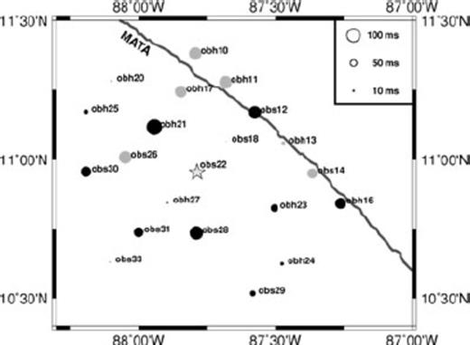
P-wave station corrections terms calculated and applied in the final iteration of VELEST. Black circles denote negative values and hence early arrivals; grey circles denote positive values (late arrivals). The star denotes the reference station obs22. Station corrections may contain contributions of both, the geological subsurface structure and the neglect of station elevations. MATA stands for Middle America Trench Axis.
4.1.2 S-wave data
In most earthquake location routines the S-wave velocity model is constrained by assuming a constant Poisson-ratio, even though it has been shown that focal-depth errors may be twice as large compared to the errors using only P-phases (Maurer & Kradolfer 1996). However, a well-constrained and independent S-wave model can contribute to the hypocenter locations and can increase the accuracy of focal depths, but it is much more difficult to pick the arrival of an S-wave than to pick a P-phase, since the onset of the S-wave most likely occurs within the P-wave coda and therefore is often covered or distorted. Regardless of a small rms fit, wrongly picked S-wave arrival times can easily cause a wrong hypocenter solution. Furthermore, only events of good quality can be included into the calculations. Thus, at least eight P-wave and four S-wave observations are required. A further requirement is that the gap in the azimuthal distribution of stations is <180°. In our data set only 18 events fulfilled these terms, which is rather a too small number to calculate an accurate S-wave minimum 1-D velocity model. Existing seismic wide-angle data of the study area (Ivandic 2008; Ivandic et al. 2008) suggest a Vp/Vs-ratios of 1.7–2.0 for the oceanic crust and 1.7–1.8 for the upper mantle. We used these values to construct a S-wave 1-D velocity model for the final hypocenter location procedure. However, the sediment cover introduces an additional problem, since the Vp/Vs-ratio can be very large and thus S-wave arrivals would be delayed. The sediment layer in the study area however shows a rather uniform thickness of ∼400 m with P-wave velocities of 1570–2100 m s−1 (Kimura et al. 1997). For such low seismic velocities it can be assumed that seismic rays emitted from earthquakes in the mantle and crust travel almost vertical in all sedimental layers. Thus, if a low Vp/Vs-ratio is used in the inversion model-even though a high Vp/Vs-ratio is actually the case for the sediments-it will mostly affect S-wave station correction terms instead of the travel time residuals. Further, the uniform sediment in the study area should lead to uniform correction terms.
We determined this station correction by using the delay time between the first P-wave arrival as seen on the Z-component and the onset of the converted SP-wave from the crust/sediment boundary as seen on the horizontal components (see Fig. S1 in the supporting information). For every obs-station this delay was found to be exactly 1.5 s. Thus, in our S-wave velocity model we give a Vp/Vs-ratio of 1 for the sediment and add a positive station correction (late arrival) of 1.5 s for all stations. The advantage of this method is, that the S-wave velocity structure of the sediment must not be known for the hypocenter location procedure.
In all further considerations, only S-waves picks from stations, which were part of a seismic wide-angle profile (cp. Fig. 1) have been included: if the OBS was tilted on the ocean floor, the horizontal components might be affected by P-waves, which may distort the onset of the S-wave. Airgun-shots have been used to rotate the seismometer components such that P-wave influence was removed from the horizontal traces. This is necessary to allow a clear picking of the S-wave onset.
4.1.3 Final hypocenter location
Final hypocenter parameters for all earthquakes are determined using the earthquake location program NonLinLoc (Lomax et al. 2000, 2001) and the final P- and S-wave 1-D velocity models (Fig. 3c).
NonLinLoc is a non-linear traveltime calculation code that produces an optimal hypocentre, a misfit function and an estimate of the probability density function from seismic phase time picks.
Further, NonLinLoc allows for 3-D velocity model, which can be used to account for station elevations. Therefore, existing multibeam bathymetry of the study area (Ranero et al. 2003) provided the water depths for a xy-grid that covers the entire network with a step size of 5 km × 5 km. Next, the final P- and S-wave 1-D velocity models (Fig. 3c) was applied beneath every gridpoint. We used this pseudo-3-D velocity model to produce accurate hypocenter parameters (Figs 5 and 6), statistical error ellipses (Fig. 6) and to determine and apply station correction terms (Fig. 7). The latter is done by running NonLinLoc without any station corrections and calculating the mean of traveltime residuals. Since station elevations are accounted for, these terms should reflect the geological subsurface structure, time-shifts of the OBS-clocks (see Supporting information) and eventual local velocity anomalies.
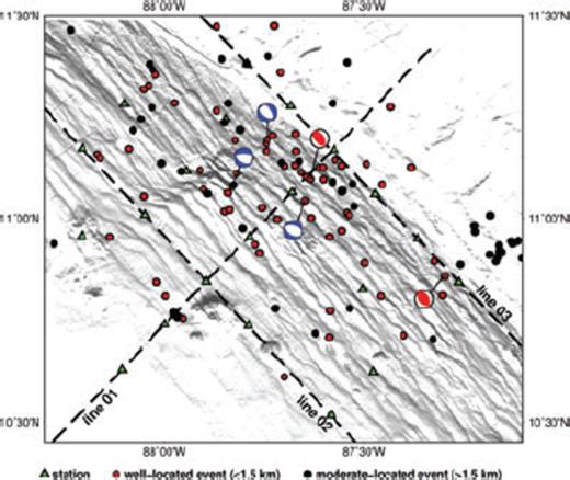
Final epicenter distribution. Locations for events used in the inversion with VELEST (red circles) are constrained with more confidence than additional sources (black circles). Error ellipses are not plotted to maintain straightforwardness. Line 01–03 show seismic wide-angle profiles (Ivandic et al. 2008) that have been used to determine crustal velocities. Focal mechanisms have been calculated using the beneath described waveform forward modelling scheme.
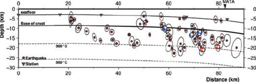
Projection of all sources that have been used for the calculation of the minimum 1-D velocity model on a cross section along line 01 (cp. Fig. 5). Isotherms are calculated using the code of McKenzie et al. (2005). ‘MATA’ denotes the Middle America Trench Axis. Statistical error ellipses are calculated with NonLinLoc. Depth denotes depth beneath sea surface in this case.
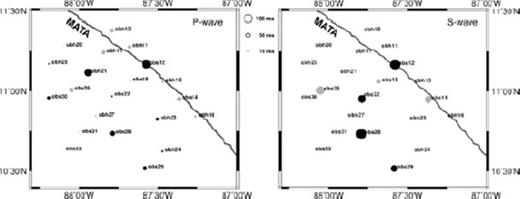
Mean of travel time residuals for P- and S-wave data (observed values minus results from the inversion), calculated and applied like station correction terms during the earthquake location procedure with NonLinLoc. Black circles denote negative values; grey circles denote positive values. Since station elevations have not been neglected, the correction terms should rather reflect the geological subsurface structure and eventually local variances from the minimum 1-D velocity as well as possible time shifts on the OBS-clocks.
The final all-over rms of all P-phases is with 196 ms slightly reduced compared to the final value with VELEST (205 ms). Hypocenter parameters vary only little between the different calculations, whereat epicentres changes are <1 km and changes of the focal depths are <2.5 km (Fig. S2) and hence within the error margins.
Additionally, we calculated epicentres for several earthquakes that were excluded from the inversion procedure for quality reasons, thereby adding every event with a gap of ≤ 300° that has been observed at least at six stations. A total number of 23 events have been added to the final data set (Fig. 5, moderate-located events).
4.2 Focal mechanisms from moment tensor determination
A seismic source can be described as a sequence of point sources on a planar fault. Both the number of point sources that are needed to reflect the rupture process and the dimension of the planar fault increase with the earthquakes magnitude, but the assumption of only one point source is sufficient to determine overall fault mechanism and centroid depth of the entire fault motion (Yamanaka & Kikuchi 2003). Since focal depth and mechanism are the parameters of interest in our study, we described the rupture process of each considered event as a single point source, which in turn can be described as a moment tensor.
We calculated synthetic seismograms for six independent elements of the moment tensor (see supporting information) using the computer routine QSEIS (Wang 1999), which is based on the reflectivity method (Fuchs 1968; Fuchs & Müller 1971; Müller 1985; Ungerer 1990). The advantage of this code is that it calculates next to the common displacement and velocity seismograms also volume changes for hydrophones. We used the results of the P-wave minimum 1-D velocity model (Fig. 3) as input for both, source and receiver site. Density structure is given in Table S2.
Moment tensor solutions were determined by comparing synthetic seismograms with observed waveforms (nominal response was removed from the observed waveforms following Thölen (2005)) using via a two-step grid search: The first step included a search over all strike angles with a step size of 10°, over all dip angles with a step size of 5° and over all rake angles with a step size of 10°, where the best-fit solution is given by the lowest variance reduction (VR) between observed and synthetic waveform. Once a best-fit mechanism was found, we refined the search using a step size of 1° for all angles starting from –20° and going to +20° relative to the best-fit solution of the first step. Both, synthetic and observed waveforms have been filtered using a 3 to 25 Hz bandpass. Beneath and respectively above these values, observed seismograms were dominated by noise.
A stable and reliable focal mechanism solution requires data of much higher quality than for the calculation of a minimum 1-D velocity model. In our experience just events with at least 10 P-wave observations and a gap in the azimuthal distribution of stations of <90° can be used.
Only 11 events from the data set fulfill these high standards, but most of them occurred in the crust, which is of secondary importance for this study. For five events in the mantle we could determine focal mechanisms. For the calculation of these focal mechanisms we used only hydrophone data, since these usually provide a better signal-to-noise ratio than the vertical seismometer components.
We chose a time window of 0.1 s before the first arrival to 0.5–0.8 s after P-onset. The window needs to be this short since the calculation of the following multiples and reflections would require a velocity model much more accurate than it can be derived from P-wave picks of local earthquakes alone.
Fig. 8, supporting Figs S3 and S4 show waveform fits between observed and best-fit synthetic data for upgoing, tensional mechanisms and Fig. 9 and supporting Fig. S5 for downgoing, compressional ones. The VR values were between 0.9 and 0.55 for the first 0.3 s after the P-wave arrival. The small 0.3 s window mostly includes the full first amplitude. Thus, the achieved VR values are good for data of such high frequencies.
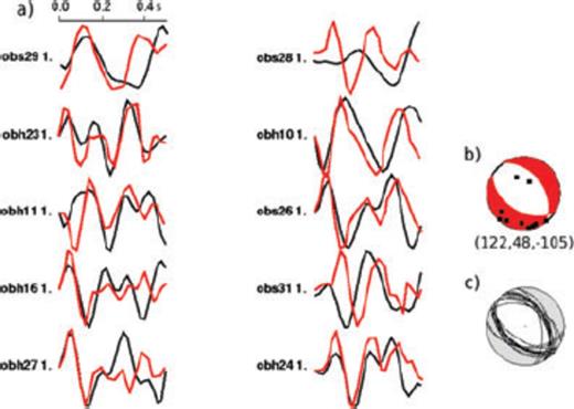
Results of the forward modelling procedure for a normal fault event. (a) Comparison between observed (black lines) and best-fit synthetic waveforms (red lines). The number behind the station name gives the weighting. Time scale shows onset of P-waves. (b) Best-fit focal mechanism and station distribution (black dots). The numbers below the mechanism diagram give the strike, dip and rake angles in degree. (c) All solutions until VR increased by more than 10 per cent.
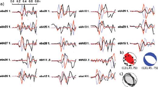
Results of the forward modelling procedure for a thrust fault event. (a) Comparison between observed (black lines) and best-fit synthetic waveforms (red lines). Blue lines show synthetic waveforms for a normal fault earthquake with equivalent strike and dip angle (blue mechanism in b), to underline that only a compressional (thrust fault) event fits the data set. The number behind the station name gives the weighting. Time scale shows onset of P-waves minus 0.2 s. (b) Best-fit focal mechanism (red) and station distribution (black dots). The numbers below the mechanism diagram give the strike, dip and rake angles in degree. The blue mechanism was used to calculate synthetic seismograms of a normal fault event (compare a). (c) All solutions until VR increased by more than 10 per cent.
The best solutions are shown in Figs 8c and 9c. Plotted are all solutions until the residual increased by more than 10 per cent. The waveform observed at a receiver is strongly influenced by the depth of the source. We carried out several grid searches using Green's functions for various source depths. The lowest residual determines the focal depth. Differences between focal depths obtained with this method and obtained from the travel time hypocenter location are ≤ 2.2 km (see Table S3 in supporting information).
4.3 Magnitudes
Following the approach of Tilmann et al. (2008), we used hydrophone traces for the calculation of moment magnitudes. We removed the nominal response following Thölen (2005). Next, the corrected hydrophone trace is multiplied by the sound velocity (1.5 km s−1) and the density of water (1000 km m−3). The resulting trace is an approximation of the displacement for a vertically incident wave and zero impedance contrast between seafloor and water. This approximation is reasonable, since velocities and densities of the uppermost sediments are comparable to that in water and cause earthquake arrivals to have steep ray paths below the station.
The calculation of moment magnitudes then was done by applying standard method and code of Ottemöller & Havskov (2003), which searches for the combination of seismic moment M0 and corner frequency f0 that fits the observed spectra the best. Moment magnitudes are calculated for every single station. Final Mw-values (Fig. 10) are the arithmetic average of all stations, error bars show the standard deviation. We used different Quality factors from QP = 300 to 600 with a slight assumed frequency dependence following Ottemöller & Havskov (2003) to evaluate the attenuation dependence. Error bars in Fig. 10 include differences from these calculations.
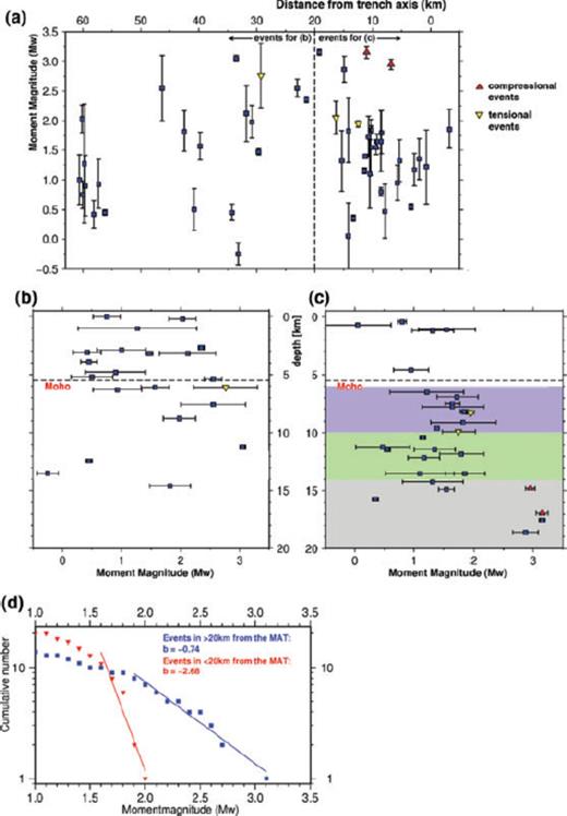
Results of the moment magnitude calculation. (a) Distribution of moment magnitudes along a profile (line 01, cp. Fig. 5) perpendicular to the trench axis. (b) Distribution of moment magnitudes with depth for events in >20 km distance from the trench axis and (c) in <20 km distance, respectively. The meaning of the colour-shaded areas in (c) is: the purple area shows a scalar seismic moment of 8.1 × 10¹¹ Nm km−1; the green-shaded area a scalar moment of 4.1 × 10¹¹ Nm km−1; the grey area a scalar moment of 29.1 × 10¹¹ Nm km−1; (d) b-factors for all events. ‘MAT’ denotes the Middle America Trench Axis. Bending points of the red and the blue line differ slightly from each other, which indicates the catalogue for events close to the trench (red line) is more complete. Most likely this is due to the higher density of seismic stations close to the trench (cp. Fig. 1).
The absolute magnitude may differ from moment magnitudes derived from well calibrated landbased seismometers. However, the only event that was recorded on- and offshore was an event with Mw = 2.8 ± 0.1. The Nicaragua earthquake service INETER estimated its magnitude with ML = 3.2, suggesting that our magnitude scale roughly compares with the INETER scale. Furthermore, we like to point out that for our investigations relative magnitudes within the recording network are more important than absolute ones.
Distribution of moment magnitudes as a function of distance from trench axis and depth respectively for 50 local events as well as b-factors are shown in Fig. 10. One feature is that in the close proximity of the trench (<20 km distance) the lithosphere seems to rupture more frequently, but under the release of less energy, that is the b-factor increases strongly, implying that the rheology of the lithosphere is changed drastically. Further, this change occurs abruptly at ∼15–20 km distance from the trench axis. Within 20 km of the trench, only relatively deep earthquakes with a compressional fault mechanism show comparable large moment magnitudes.
5 Discussion
The epicentre distribution of local earthquakes (Fig. 5) fits the strike direction of bending-related faults imaged in bathymetric data. Furthermore, seismicity increases toward the trench axis. Both features suggest that trench-outer rise seismicity is related to plate bending. Seismic reflection data (Ranero et al. 2003) and focal solutions of large trench-outer rise earthquakes recorded at teleseismic distances (Lefeldt and Grevemeyer 2008) suggest that bending-related faults dip landwards at an angle of ∼40°–45°. Focal mechanisms derived in this study show dip angles of 40° to 51° (see Table S2 in supporting information) and thus coincide with previous studies. Seismic events were exclusively recorded in areas that show faulting in the bathymetry (up to 60 km seawards the trench) and earthquakes reach approximately 15 km into the mantle. The number of earthquakes increases toward the trench, but the deepest events were recorded roughly 20 km seaward of the trench axis. Seismic images (Ranero et al. 2003) suggest that normal fault related to bending reach 10–15 km into the mantle, which coincides with the results of this study and previous estimates (Grevemeyer et al. 2007).
However, large or moderate (teleseismic) earthquakes might be able to cut deeper into the lithosphere, but such events were not recorded within the network during the period of deployment. Focal mechanisms, centroid depths, and dimensions of rupture areas obtained from large trench-outer rise earthquakes occurring within the study area suggest shallow focal depths (<25 km) and fault planes of low aspect ratio, that is a dimension of 40–50 km in strike and 5–15 km in dip direction (Lefeldt & Grevemeyer 2008). Thus, such events may indeed exceed depth limits revealed for microseismicity in this study, but they may not be representative for the typical cutting depth of bending-related faulting: Several studies suggest (Chapple & Forsyth 1979; Lefeldt & Grevemeyer 2008; Ammon et al. 2008) that trench outer rise normal fault earthquakes of moderate or large magnitude (Mw > 5.0) are slab-pull related, that is occur after large interplate thrust earthquakes have reduced the degree of coupling between the oceanic and the continental plate. Thus, a normal faulting intraplate event occurs in the moment the gravitational slab-pull stress is transferred into the outer rise (Ammon et al. 2008). After failure, tensional stresses in the incoming lithosphere are again reduced, that is the neutral plane is shifted upwards. Thus, time between the arrival of tensional slab-pull stress at the outer rise and the release of this stress in a moderate or large normal fault event might be comparable short. Note, that the tensional stress transfer from the slab after the decoupling of the plates due to a large thrust fault event must not be quick, but can be of viscoelastic nature and might take several month (Ammon et al. 2008).
Two moderate sized earthquakes ruptured the area eight and 12 months after the ORN was recovered. Parameters for these events (Global Centroid-Moment Tensor solution catalogue GCMT, http://www.globalcmt.org/CMTsearch.html) are: date = 7/25/2006; Mw = 5.0; strike = 119(313)°, dip = 43(48)°, rake = −100(−81)° and date = 11/18/2006; Mw = 5.5 strike = 128(301)°, dip = 47(43)°, rake = −85(−95)°. The long period between the recovery of the ORN and the occurrence of moderate normal fault events in the area suggest that horizontal stresses at the time of deployment of the ORN where rather governed by the coupling between the overriding and the subducting plate than by the gravitational slab-pull. Supported is this by bending-models for the oceanic lithosphere after Chapple & Forsyth (1979) and Christensen & Ruff (1988), which propose that earthquakes with compressional fault mechanisms-as observed in our data set-are caused by the horizontal stress of the plate coupling only and thus are exclusively observed in the coupled state. Further, 1 week before the recovery of the ORN, a moderate interplate thrust fault event occurred (date = 08/11/2005; Mw = 5.9; strike = 282(121)°, dip = 19(72)°, rake = 72(96)°). This event might have decreased the degree of coupling, which than led to a slow transport of slab-pull stress to the outer rise-causing a normal fault rupture 8 months later.
We therefore assume that the stress distribution, as derived from moment tensor analysis in our study, represents the coupled state. We found tensional earthquake in our data set up to depths of 9.9 ± 1.7 km below seafloor (see Table S2 in supporting information, Fig. S6), whereas the shallowest compressional earthquake was found at 14.8 ± 2.1 km below seafloor. Confidence that the deep earthquakes are indeed compressional comes from a comparison of different possible focal mechanisms (Fig. 9). Synthetic waveforms calculated with a compressional focal mechanism fit the observed waveforms, whereas an assumed tensional mechanism obviously does not. Thus, we observe indeed a transition from tensional to compressional stresses with a neutral plane located at ∼12 ± 2 km below seafloor, which is relatively shallow. Most likely water cannot penetrate into an area governed by compressional stresses and hence the neutral plane could present a barrier and thus might be the important parameter for the depth of outer rise mantle hydration.
McKenzie et al. (2005) suggest that the 650 °C isotherm marks the thermal limit at which earthquakes are observed. Previous studies (e.g. Ranero et al. 2003) based their interpretation on this idea and proposed that fluid transport and hence serpentinization occurs until the thermal limit of serpentinite at ∼600 °C is reached. The only study that used local outer rise earthquake data prior to the present one found seismic activity in the oceanic plate offshore southern Chile down to temperatures of 500–600 °C (Tilmann et al. 2008). Off Nicaragua, most microseismicity occurs above the 300 °C isotherm (Fig. 6). Both studies might not be comparable since the Chilean network was deployed on much younger oceanic plate of ages 14 million of years ago and 6 million of years ago, respectively.
However, the remaining question is: does fluids infiltrate indeed through the tensional fault system into the mantle, causing serpentinization? The final minimum P-wave 1-D velocity model shows velocities of 7.4–8.1 km s−1 million of years ago (average 7.8 km s−1) in the upper 10–12 km of the mantle, which is 1–9 per cent (average 4.5 per cent) lower than expected values for unaltered peridotite in this area (Ivandic et al. 2008). Reduced seismic velocities can be explained by a partly serpentinized mantle (Carlson & Miller 2003). Such velocity anomalies are as well observed in seismic wide-angle and refraction data (Grevemeyer et al. 2007; Ivandic et al. 2008; Ivandic 2008) and indicate a fractured and serpentinized mantle. The depth of this velocity anomaly shows an increasing evolutionary trend toward the trench.
If velocities are indeed decreased by serpentinization, we can use the derived P-wave velocities to estimate the amount of stored water in the mantle: following Carlson & Miller (2003), the degree of serpentinization and water content of partially serpentinized peridotites can be related to the P-wave velocity. Using their formula, we estimate 1.4 weight per cent water stored in this area, which would correspond to 11 per cent of serpentine in the mantle.
This is an upper limit for the case that the low velocities are exclusively caused by serpentinization. Indeed, cracks-like the bending-related faults-should lead to lower velocities as well, especially for rays that travel perpendicular to them. Note, that this result is calculated from the 1-D velocity model, which gives only an average of the whole area. Since seismic velocities seem to decrease toward the trench (Ivandic et al. 2008), serpentinization could be higher.
However, it is difficult to evaluate the accuracy of the final 1-D velocity model and further, an evolutionary trend of a reduced velocity anomaly would require at least a 2-D velocity model. Nevertheless the latter might be observed through the station corrections (Figs 4 and 7). Close to the trench mostly positive station corrections are observed, that is a late arrival, meanwhile negative station corrections (early arrivals) prevail in greater distance. This cannot be an effect of the neglect of station elevation, since in this case the deeper stations close to the trench should show early arrivals. Rather this feature may reflect the evolutionary trend of reduced velocity anomalies toward the deep sea trench, as observed in seismic refraction data (Ivandic et al. 2008).
A strong argument for fluid infiltration and perhaps serpentinization comes from the determination of moment magnitudes and b-factors (Fig. 10). Toward the trench, the number of earthquakes per unit length increases significantly (Fig. 10a), whereas moment magnitudes decrease. At greater distance (>20 km from the trench axis), moment magnitudes are distributed randomly with depth (Fig. 10b). In contrast, in the close proximity of the trench, larger magnitudes of Mw > 2.0 are only reached in the compressional area (Fig. 10c). Thus, within 20 km of the trench axis rupture seems to be much more frequently, though the release of energy per event is low. Here, the b-factor is with b = 2.68 extraordinary large, which implies a lithosphere of weak rheology. The transition from strong to weak seems to occur abrupt at ∼20 km distance from the trench axis (Fig. 10). This behaviour could be interpreted using results from laboratory experiments on hydrated mantle rocks (Escartín et al. 2001). When peridotite is serpentinized by more than 10 per cent, its rheology changes abruptly from ‘pure peridotite’ to ‘pure serpentinite’, suggesting that the upper mantle is indeed partly serpentinized.
Further, the neutral plane at 12 ± 2 km depth beneath seafloor can be seen as well in the distribution of moment magnitudes. Commonly, it can be assumed that seismicity becomes low around the neutral plane, which can be directly observed here: in close proximity to the deep sea trench, moment magnitudes and hence seismicity are lower between 10 and 14 km beneath seafloor than above and beneath (Fig. 10c, scalar moment per km is two times smaller at 10–14 km than above and eight times smaller than below). In contrast, the distribution of micro-earthquakes seems to be uniform with depth (Fig. 6). This suggests that the lithosphere fractures the same frequently around the neutral plane, where stresses are comparable low, which is another indication that the mantle is of weak rheology.
6 Conclusion
Microseismicity at the trench-outer rise offshore Nicaragua is restricted to the upper ∼12 km of the mantle. However, events of large magnitude (Mw > 5), which have not been observed during the duration of deployment, might cut to greater depth, but are mostly slab-pull related and thus temporarily very limited events.
A change of the stress regime occurs roughly at 6 km below Moho, changing from tensional above to compressional beneath. The intersection between both regimes could present a barrier for sea water, which cannot penetrate any deeper.
In consequence, all values for possible serpentinization in this area, which mostly were derived from the depth of the bending-related faults (e.g Ranero et al. 2003) need to be scaled down. Seismic velocities from the P-wave minimum 1-D-model suggest, that >10 perxs cent of serpentine could occur in the upper most 10 km of the mantle.
Moment magnitudes suggest an abrupt change of the rheology of the lithosphere from strong to weak at ∼20 km distance from the trench axis. Such a change could occur when a degree of serpentinization of ∼10 per cent is reached.
Acknowledgment
The ORN was deployed and recovered during R/V Meteor cruises M66/3 and M66/4. We thank scientific participants and crews for their efforts and officers for their technical and logistical support. The cruises were founded by DFG. This work is contribution no. 114 of ‘SFB 574-Volatiles and Fluids in Subduction Zones: Climate Feedback and Trigger Mechanisms for Natural Disasters’ from the University of Kiel and IFM-GEOMAR, Kiel. We would like to thank Masanao Shinohara from the University of Tokio and one anonymous reviewer for their very useful comments and indications.
References
Supporting Information
Additional Supporting Information may be found in the online version of this article
Appendix S1. Supplementary tables and text referenced in the main body of the article.
Please note: Wiley-Blackwell are not responsible for the content or functionality of any supporting information supplied by the authors. Any queries (other than missing material) should be directed to the corresponding author for the article.
