Estimation of crustal scattering parameters with elastic radiative transfer theory

Summary

1 Introduction

For modelling of elastic wave energy propagation through the Earth's crust, radiative transfer theory (RTT) can be used. RTT describes the propagation of wave energy in scattering random media. Phase information is neglected, and it is assumed that wave energy is incoherent. In applications to real data, squared seismogram envelopes, which are proportional to the energy density of waves, are usually considered.

Originally, RTT was introduced to describe the transport of light through atmospheres (e.g. Chandrasekhar 1960). RTT is a so-called ladder approximation of the Bethe—Salpeter equation. This approximation works well if (1) wavelengths are comparable to correlation length, (2) fluctuations of the inhomogeneities are weak and (3) macroscopic features of the propagation medium are large compared with the wavelength (high frequency approximation; Papanicolaou et al. 1996).

In seismology, RTT was mostly used in the approximation of isotropic acoustic scattering to separate intrinsic and scattering attenuation (e.g. Hoshiba et al. 1991; Sens-Schönfelder & Wegler 2006). Anisotropic acoustic scattering approximation (e.g. Gusev & Abubakirov 1987, 1996; Wegler et al. 2006) is more realistic than isotropic scattering because envelope broadening can be modelled. So far, most applications are based on acoustic RTT and rely on the fact that due to conversion scattering, S-waves rapidly become dominant in the coda part of the seismogram (Aki 1992).

In elastic RTT, P- and S-wave modes are included and mode conversion is taken into account (e.g. Zeng 1993; Sato 1994; Margerin et al. 2000; Margerin & Nolet 2003; Shearer & Earle 2004; Przybilla & Korn 2008). With anisotropic RTT, a good agreement between finite difference solutions of wave equations and numerical solutions of radiative transfer equation is achieved. This has been shown for the acoustic RTT (Wegler et al. 2006) and also for the elastic RTT (Przybilla et al. 2006; Przybilla & Korn 2008).

The most recent development in seismic scattering theory is the introduction of conversion scattering between body and Rayleigh waves in the single scattering approximation (Maeda et al. 2008).

In this paper, we present the first systematic application of elastic RTT to invert scattering parameters of the Earth's crust. We find that for crustal scattering, the resolvable parameter is the transport mean free path (TMFP). We demonstrate that only a certain parameter combination of fluctuation strength ɛ and correlation length a is resolvable, depending on the type of autocorrelation function of the random medium. Finally, we show results of an inversion of scattering parameters from seismograms of a local earthquake in Norway.

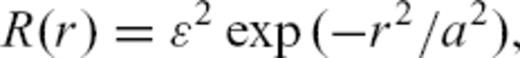
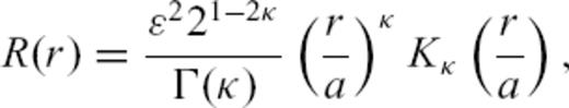
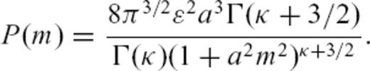
2 Random Media

Continuous random media are models for small scale heterogeneities in Earth structures. They are characterized by their autocorrelation function R. We use homogeneous and isotropic random media where R only depends on the absolute value of distance r = ǀrǀ. The two most important parameters of an autocorrelation function are, fluctuation strength ɛ and correlation length a. ɛ gives the fluctuation of velocities around a mean value, and a gives the spatial variation of this fluctuations. Typical types of autocorrelation functions R and their Fourier spectra P for Earth heterogeneities are the Gaussian random medium

1

2

and the von Karman random medium (Sato & Fehler 1998, p. 14)

3

4

Here the power spectral density function P(m) is the Fourier transformation of the autocorrelation function R(r), r is spatial distance, m the absolute value of the associated spatial wave number, Γ is the Gamma function and K_κ is the modified Bessel function of the second kind of order κ (Abramowitz & Stegun 1970, p. 375). At large wave numbers am ≫ 1, the power spectral density function P(m) of the von Karman medium obeys a power law, and Hurst number, κ, controls the order of the power law. This power law means that the von Karman medium is rich in short wavelength components compared with the Gaussian medium. A special case of the von Karman medium for κ = 0.5 is the exponential random medium (Sato & Fehler 1998, p. 15).

3 Radiative Transfer Theory

The coupled elastic radiative transfer equation is an integro-differential equation and is solved numerically by Monte Carlo simulations. In a Monte Carlo simulation, wave energy is represented by particles. Each particle is a bin of wave energy. Many particles yield the energy field of the wave. Particles start at the source and propagate through the medium with P- or S -wave velocity, according to ray theory. When scattering occurs, the particle changes its propagation direction and may convert from P to S, and vice versa. When particles pass a small spherical shell volume around the source, they will be counted. By averaging many particles (∼10⁶ to ∼10⁸), the energy density per time and volume is simulated. A full description of the Monte Carlo algorithm for the elastic 3-D case is given in Przybilla & Korn (2008).

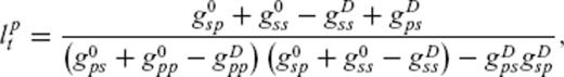
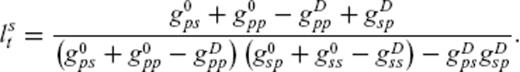
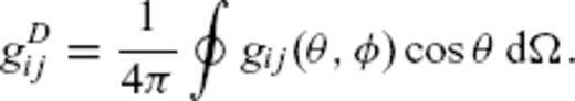
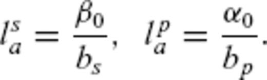
3.1 Born scattering coefficients

For the description of single scattering interactions, Born scattering coefficients are used. They are derived from the Born approximation, that is, first-order perturbations for weak fluctuations (Sato & Fehler 1998, p. 87). From a theoretical point of view, Born scattering coefficients fail if scattering is very strong in forward direction. However, as shown in Przybilla & Korn (2008), full-waveform finite difference solutions and Monte Carlo simulations in the strong forward scattering regime agree very well. Born scattering coefficients describe the power of scattered waves per unit volume and per scattering angle. In the presence of P- and S-wave modes, four scattering coefficients are needed. g_pp(θ, φ) and g_ss(θ, φ) describe P-to-P wave and S-to-S wave scattering, respectively; g_ps(θ, φ) and g_sp(θ, φ) describe conversion scattering from P to S and vice verse, respectively. Angles θ and φ give the direction of the scattered wave in spherical coordinates, when it is assumed that the incident wave propagates along θ = 0 and polarization of incident S wave is always along φ = (0, π). As an example g_pp(θ, φ) reads

5

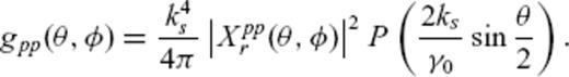
k_s is S wavenumber and γ₀ = α₀/β₀ is the ratio of P velocity α₀ and S velocity β₀. Here we use . Scattering coefficients depend on the power spectral density P of the random medium and scattering pattern X, for example,

6

Parameter ν describes the empirical proportionality of density and P-wave velocity (Birch's law) and was found to be ν = 0.78–0.82 for the Earth's crust (Birch 1961). In this paper, we use a ν = 0.8. We refer to Sato & Fehler (1998, p. 104) for the other coefficients. We can write scattering coefficients in a simplified functional form as

7

where i, j is p or s. This means that each scattering coefficient can be written as the product of parameter combination ɛ²/a and a functional F in which parameters a and k_s only occur as product ak_s. Parameter combination ak_s describes the direction dependence of scattering. If waves are scattered, then for ak_s ≪ 1 waves are scattered mainly in backward direction; but for ak_s ≫ 1, waves are scattered mainly in forward direction. For ak_s≈ 1, waves interact most intensively with the medium, which means that scattering is effective because wavelength is of the same order as correlation length of the medium.

Integrating the scattering coefficients over the full space angle, we obtain the total scattering coefficients:

8

Fig. 1 shows the dependence of total scattering coefficients g⁰_ij on parameter ak_s for different types of random media. The asymptotic behaviour of g⁰_pp and g⁰_ss with ak_s is independent of the type of random medium. They are proportional to (ak_s)⁴ for ak_s ≪ 1 and proportional to (ak_s)² for ak_s ≫ 1. Significant differences in the conversion scattering coefficients g⁰_ps and g⁰_sp exist. For a Gaussian random medium and ak_s ≫ 1, conversion scattering is negligible because conversions scattering coefficients become very small. For exponential media, it becomes independent of frequency for ak_s ≫ 1. For von Karman medium 0 < κ < 0.5 conversion scattering increases with frequency.

Figure 1.

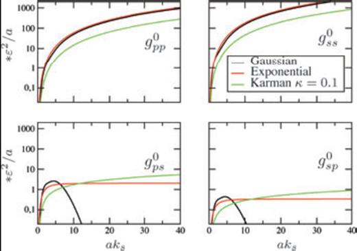
Dimensionless total elastic scattering coefficients for different random media. For a Gaussian autocorrelation function, the conversion scattering coefficients vanish in the case of strong forward scattering. That means P and S waves propagate separately without conversion between these modes.

Open in new tabDownload slide

From total scattering coefficients, we can calculate mean free paths (MFP). A MFP is the average propagation distance of waves between two scattering events. From Ryzhik et al. (1996):

9

Here l_p is MFP for P waves and l_s for S waves, respectively. MFPs are essential to build the Monte Carlo algorithm (Przybilla & Korn 2008). The other important values are the transport or effective mean free paths (TMFP) l^p_t for P waves and l^s_t for S waves. In contrast to the MFP, the TMFP is the length scale on which P and S waves are scattered out of their original direction of propagation. The TMFPs are defined as (Weaver 1990; Ryzhik et al. 1996)

10

11

with

12

From the TMFP of P and S waves, we can compute the diffusion constant D for elastic waves. It is defined as (Weaver 1990; Ryzhik et al. 1996)

13

The diffusion constant describes the behaviour of energy envelopes after many scattering events. In this limit, envelopes are identical to solutions of the diffusion equation. Fig. 2 shows the elastic diffusion constant D according to eq. (13) and the TMFPs l^p_t and l^s_t according to eqs (10) and (11), as a function of ak_s for different types of random media. Differences between l^p_t and l^s_t are negligible for strong forward scattering, and therefore D has the same frequency dependence as l^p_t and l^s_t. It is difficult to find simple analytical approximations of eqs (10) and (11) in the strong forward scattering regime. Instead, we provide the approximations obtained for l_t for acoustic waves and ak ≫ 1:

14

15

16

For strong forward scattering, l_t becomes independent of frequency for the Gaussian random medium (see Fig. 2). For the exponential medium, there exists a weak logarithmic frequency dependence. In the von Karman medium with 0 < κ < 0.5, frequency dependence of TMFP depends on the value of κ. From the frequency dependence of TMFP, we can therefore estimate the medium type and typical relations of the parameter combination of ɛ and a (e.g. in a Gaussian medium we can estimate ɛ²/a if scattering is in the strong forward scattering regime (ak_s ≫ 1).

Figure 2.

TMFP and Diffusion constant for different random media and ɛ²/a = 1 km⁻¹. For ak_s ≫ 1 frequency dependence is characteristic for each random medium. The blue curves show the acoustic TMFP approximations from eqs (14) to (16).

Open in new tabDownload slide

3.2 Monte Carlo simulations for strong forward scattering

Now we study Monte Carlo simulations in the strong forward scattering regime ak_s ≫ 1, as apparently high frequency seismic waves seem to be mainly in strong forward scattering regime, because broadening of seismogram envelopes is often observed (e.g. Sato 1989; Saito et al. 2002). In Fig. 3, Monte Carlo simulations for different random media types and two values of ak_s are shown. TMFP is l^s_t = 100 km in all simulations. As all terms in eq. (11) have the functional form like eq. (7), we can numerically determine a value of ɛ²/a for fixed ak_s and l^s_t. This value is then used in the Monte Carlo simulations. Envelopes at three radial distances r = 0.5 l^s_t, l^s_t and 1.5 l^s_t are plotted. In all graphs, the first peak is the P-wave onset and the second is the S-wave onset. Behind these peaks, codas appear.

Figure 3.

Monte Carlo simulations for two values of ak_s in three different random media (columns) and for three different distances (rows). Simulations are done with the same value of TMFP of l^s_t = 100 km. Differences between envelopes for different ak_s are clear in the Gaussian medium but very small in the case of other media.

Open in new tabDownload slide

In the Gaussian medium, there is strong difference in the P coda between ak_s = 8 and ak_s = 16. The conversion coefficients become very small in the Gaussian medium (Fig. 1). So, the sagged P coda for ak_s = 8 goes to an exponential like decreasing P coda for ak_s = 16. It follows that P and S waves propagate independent of each other, and we obtain a sharp transition between P coda and S-wave onset. This sharp transition remains for higher values of ak_s > 16. The envelope after S-wave onset remains similar for both values of ak_s.

In the exponential medium, we find the biggest difference between both simulations in S coda for distances smaller than TMFP. Here we have an influence of conversion scattering in the strong forward scattering regime too.

In von Karman medium with κ = 0.1, there is no clear difference visible. There are only small differences between the simulations for both values of ak_s in exponential and von Karman medium. This means that in the case of strong forward scattering, the envelope shape in a random medium for a distance r mainly depends on the TMFP.

Typical for envelope shapes in the strong forward scattering regime is envelope broadening for waves that are mainly forward scattered (near P- and S-wave onset) and a sagged S coda that is clearly visible in the Gaussian medium for distances smaller than TMFP. This sag of the S coda comes from the scattering nearly in propagation direction of waves. In summary, we can say that in the strong forward scattering regime, the dependence of envelopes on parameter ak_s is weak and the shape of envelopes mainly depends on TMFP. Therefore, in the strong forward scattering regime, we expect that only TMFP can be inverted from real data, whereas parameter ak_s is difficult or impossible to resolve.

4 Data Example

As a data example, we use the of 2004 April 7 M_L = 3.5 Flisa earthquake, UMT 08:53:20.0. It occurred near the NORSAR array in southern Norway (Fig. 4) at 22.5 km depth (Schweitzer 2005). Therefore, we expect that, mainly, body waves are generated. The hypocentral distances are between 50 and 100 km. For this distance range, the influence of Moho reflections is not so strong compared with larger distances. So, a simple full space model is a reasonable approximation.

Figure 4.

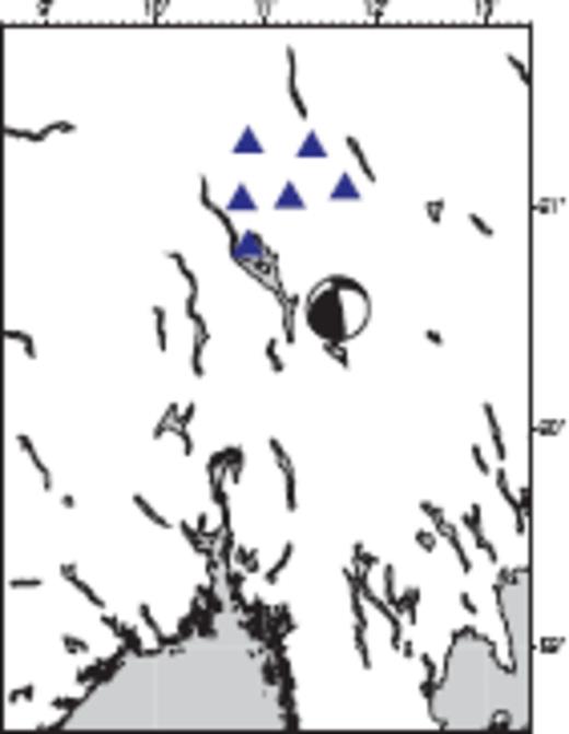
Location of the Flisa earthquake and the six used stations of the NORSAR array.

Open in new tabDownload slide

4.1 Data processing

Three-component broad-band data of six stations were processed. We used Butterworth bandpass filters of order 2, with centre frequencies of f_c = 2, 4, 6, 8 and 10 Hz, with a bandwidth of 2 Hz. After filtering, squared envelopes of each component are computed, and all three components are stacked to obtain data envelopes that can be compared with mean squared envelopes of Monte Carlo simulations. All envelopes are normalized by average energy in a time window of t = 275–300 s. With this normalization, we minimize the influence of site effects for different stations.

4.2 Forward modelling

To apply a stochastic theory based on ensemble averages to data of a single realization of the Earth, we need ergodicity. This means that we assume that time and/or spatial averages of the stochastic process can be used as an approximation for the ensemble average. For a general stochastic field ξ (Apresyan & Kravtsov 1996, p. 156), we get

17

Here is the time average of ξ(t′), 〈ξ〉 is the ensemble average and is the spatial average. Here we use the squared seismogram envelopes as an approximation for the stochastic field ξ. We obtain spatial averaging due to the use of receivers in different distances and angular directions from the source, although the azimuthal range is limited to about 60°.

The time averaging is realized by using time windows of length T = 7 s with 50 per cent overlap, which is large enough to build an average but small enough to see differences between data and simulation envelopes near the P- and S-wave onsets. We compare simulated and data envelopes from P-wave onset up to a lapse time of 300 s, limited by a minimum signal to noise ratio of 4, estimated between S coda and envelope before P-wave onset, in a time window of 7 s.

Fig. 5 shows data envelopes for three frequencies at one station (NC3). The envelope in the 2 Hz band has a strongly sagged S envelope, but envelopes at higher frequencies show an almost exponential decrease. This sagged S envelope shows that waves must be in a strong forward scattering regime at distances shorter than TMFP (see Fig. 3). In Fig. 3, we see a sagged S envelope, especially for the distance r = 0.5l^s_t. In the Monte Carlo simulations, for computational reasons, we use an isotropic radiating source with an energy ratio of W^s₀/^p₀ = 23.5, corresponding to a DC source in a Poisson solid (Sato & Fehler 1998). The observed DC has an orientation as shown in Fig. 4. If we compare the time integrals of data envelopes near the P- and S-wave onsets, we get a ratio of W^s₀/^p₀≈ 20, near the theoretical ratio.

Figure 5.

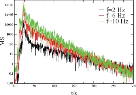
Data envelopes of station NC3 of the NORSAR array in three frequency bands normalized to the time average between t = 275 and 300 s. Envelope for f_c = 2 Hz shows a clearly sagged S coda compared to the almost exponentially decreasing envelopes at higher frequencies.

Open in new tabDownload slide

We search for scattering parameters with a grid search procedure. Scattering coefficients depend on wave number k, on parameters a and ɛ and on the type of random media. In von Karman media, an additional dependence on parameter κ exists. From Fig. 3, we found that for the strong forward scattering regime, the dependence on parameter ak_s is weak for the same values of TMFP. Therefore, we build the grid search in such a way that parameter ak_s varies in the range 1-32 in steps of ak_s = 1, 2, 4, …, 32. ɛ²/a is sampled such that TMFP varies from l^s_t = 50 to 1000 km. Data envelopes E_D and Monte Carlo envelopes E_M are connected by

18

Here W^j is an energy factor of station j and b^j is intrinsic absorption. T_k is centre time of time window k. Intrinsic absorption of wave energy density E is contained in absorption constant b. Here we put intrinsic absorption of P and S waves equal, as b_p = b_s = b. So, we can estimate intrinsic absorption with a least-square method. Otherwise, we would have to perform a grid search for intrinsic absorption, too. The assumption of equal absorption constants for P and S waves is a bit arbitrary. However, the absorption effects will be most visible at long lapse times, that is, within the S coda, which is mostly composed of S-wave energy. Therefore, b will mostly be a measure for b_s.

The inversion problem is partly linearized by taking the logarithm of eq. (18):

19

Now, we get the energy factor W^j and the absorption factor b^j for each station from a simple least-square method. We average W^j and b^j over all M stations to get average values W and b:

20

21

We now estimate the misfit e between the Monte Carlo simulations and data through

22

Here N is number of time windows. For an error measure, we use the F-test with 95 per cent confidence interval.

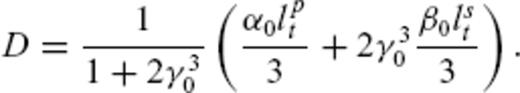
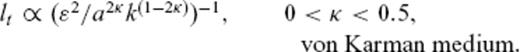
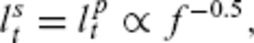
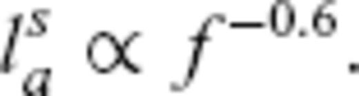
To estimate κ of the von Karman medium, we took the following approach to avoid a computationally expensive grid search on κ: in a preliminary step, we performed an inversion for the S coda part of the envelopes with an analytical approximation by Paasschens (1997), which is based on acoustic isotropic scattering. The same inversion strategy as described above has been used. As a result, a frequency dependence of TMFP as l_t∝f^−0.6 was obtained, yielding κ = 0.2 (eq. 16). This value of κ is then used as a fixed parameter in the full inversion based on Monte Carlo simulations of elastic RTT. Additional support for this choice comes from Flatté. & Wu (1988), who showed that neither a Gaussian nor an exponential random medium is a good estimation for the crustal structure under NORSAR.

In Fig. 6 and 7, best fits from the full elastic inversion are shown for frequencies 2 and 10 Hz. The influence of source radiation pattern can be seen in the 2-Hz-frequency band. There is a minimum in P-energy radiation at station NB2 and NC3. For 10 Hz, the influence of source radiation pattern is not visible anymore.

Figure 6.

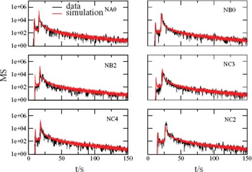
The six panels show the best Monte Carlo fits to data in the f_c = 2 Hz frequency range. All six (NA0, NB2, NC4, NB0, NC1, NC2) stations are plotted. Distance is increasing from top to bottom and from left- to right-hand side.

Open in new tabDownload slide

Figure 7.

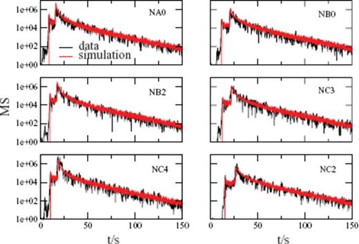
Same as in Fig. 6 but for the f_c = 10 Hz frequency range.

Open in new tabDownload slide

Misfit functions e for different values of ak_s are shown in Fig. 8, plotted against the parameter value ɛ²/a^0.4. In all frequency bands, we obtain nearly the same value for ɛ²/a^0.4 = 2 × 10⁻³ km^−0.4 at the minimum of the misfit function e. The minimum is found for the maximum value of ak_s = 32, but the difference is very little compared with ak_s = 16 and ak_s = 8. This means that the correlation length a of the crust has a large value, so that we find the minimum of the misfit function at the maximum value of ak_s = 32. Higher values of ak_s cannot be simulated with the Monte Carlo method because of long simulation times. However, higher values of ak_s are not resolvable as seen in Fig. 3, where only small differences between the envelopes at ak_s = 8 and ak_s = 16 occur, especially in the von Karman medium. This means that if waves are in the strong forward scattering regime, the influence of parameter ak_s on the envelope shape is very little, especially in distance range greater or equal to the TMFP. In Fig. 9, the same misfit functions are plotted as in Fig. 8 but against the TMFP of S waves. The resolution of the TMFP gets better for large values of ak_s. Especially in the high frequency regime, the minimum of the misfit function is sharp. This means that the resolvability of the TMFP corresponds with the resolvability of ɛ²/a^0.4.

Figure 8.

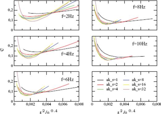
Misfit functions e for different values of ak_s in all used frequency bands against the parameter combination ɛ²/a^0.4.

Open in new tabDownload slide

Figure 9.

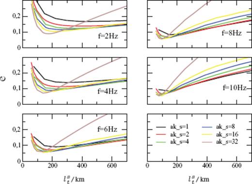
The same misfit functions e as in Fig. 8, but here against the transport mean free path l^s_t of S waves.

Open in new tabDownload slide

To compare intrinsic absorption with scattering absorption, we calculate an absorption length for S waves l^s_a and one for P waves l^p_a by using

23

The path lengths for absorption are easily converted to the Q_i-values by Q^p_i = 2πf l^p_a/α₀ and Q^s_i = 2πf l^s_a/β₀. Because the intrinsic absorption of P waves, b_p, was set to b_p = b_s in our calculations, we look further for l^s_a only.

Fig. 10 shows the dependence of TMFPs and absorption paths on frequency. In the frequency range between 1 and 6 Hz scattering, the TMFP is shorter than the absorption path. For higher frequencies both are in a similar range. TMFP of P and S waves are continuously decreasing from l^s_t≈ 200 km at 2 Hz to l^s_t≈ 100 km at 10 Hz. In a linear fit, we find

24

25

The frequency dependence of l^s_t and l^p_t approximately agrees with the assumed von Karman medium and would correspond to a value of κ = 0.25. As we can see, the frequency dependence is nearly the same as in the assumed f^−0.6. So, we think that the frequency dependence of the TMFP is affected not so strongly from the choice of the correlation function.

Figure 10.

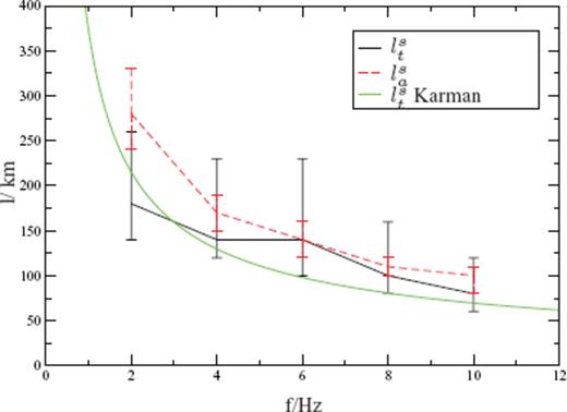
Estimated transport mean free paths l^s_t and absorption mean free path l^s_a for the Norwegian data example. For both, we find a decrease with frequency. Error bars are estimated with the F-test with 95 per cent confidence interval. The green curve shows the theoretical value for l^s_t in a von Karman medium with κ = 0.2 calculated from eq. (11) with a = 4 km⁻¹ and ɛ = 0.059 per cent.

Open in new tabDownload slide

5 Discussion And Conclusions

Monte Carlo simulations of wave energy transport through scattering media are a useful tool to compare theoretical seismogram envelopes with envelopes of seismic data. In contrast to acoustic simulations, elastic Monte Carlo simulations allow the comparison of envelopes from first P-wave onset until the late coda. This means that we can use the P coda together with the S coda.

From our Monte Carlo simulations and in the comparison with data, we find that in the strong forward scattering regime, the dependence of envelopes from parameter ak_s is weak. This implies that only TMFP is the parameter of the random medium that is resolvable (Figs 3 and 9). The importance of the TMFP as a key parameter for pulse broadening and coda envelopes was previously suggested in Gusev & Abubakirov (1996) for acoustic waves. Here we can resolve a parameter combination of a and ɛ that depends on the type of random medium and can be calculated analytically for the acoustic TMFP. This parameter combination is the same for the elastic TMFP. For our data example, we found that a von Karman medium with κ = 0.2 fits the data well and is a good model for small-scale heterogeneity of the Norwegian crust near the NORSAR array. It was found in Flatté. & Wu (1988) that in the case of a single scattering layer model a von Karman medium with κ = 0.33 fits the data better than a Gaussian or an exponential medium below the NORSAR array. That result is close to our finding.

Our data example also shows that waves with frequencies greater than 1 Hz are in the range of strong forward scattering. In strong forward scattering regime the Markov approximation can be used to simulate the broadening of envelopes. It is valid for the first part of a seismogram only. The coda part cannot calculated. Przybilla & Korn (2008) showed that the Markov approximation of elastic waves (Sato 2007) and Monte Carlo simulations agree very well at the beginning of the P- and S-wave onsets. In Monte Carlo simulations, we have the possibility to simulate the pulse broadening and the coda part of envelopes simultaneously. That makes it easier to separate intrinsic absorption from scattering absorption in Monte Carlo simulations compared with the Markov approximation. The Markov approximation was used, for example, to compare seismograms of small high-frequency earthquakes at intermediate distances (Sato 1989). It was also used in Saito et al. (2002), where random inhomogeneity parameters in northeastern Honshu Japan were estimated as a von Karman medium with κ = 0.6 and ɛ^2.2/a≈ 10^−3.6 km⁻¹.

In future work, the Monte Carlo algorithm will be expanded to more complicated geometries, for example, a scattering layer over homogeneous half-space. In such a model, there exists an exponential decay of the envelopes too. The reason for this is the leakage of energy from the crust into the mantle. Margerin et al. (1999) showed that this effect is small if the MFP is much larger than the crustal thickness. In our data example, we have seen that the TMFP is larger than the crustal thickness; and so, there is probably only a small effect of energy leakage into the mantle. Therefore, we think that for the distance range up to around 100 km from source, the full space model is a reasonable first approximation to estimate scattering parameters.

Acknowledgments

We thank the staff of the NORSAR Institute for providing data and for their friendly support. We also thank the Access to Research Infrastructure (ARI) programme for a very interesting short term stay at the NORSAR Institute. This work was supported by Deutsche Forschungsgemeinschaft (grants Ko1068/5-1,2, We 2713/2-1). Some parts of the computations were done at the John von Neumann computing centre Forschungszentrum Jülich. The authors are grateful for helpful comments to two anonymous reviewers.

References