


Summary
The Somma–Vesuvius volcanic complex and surroundings are characterized by topographic relief of over 1000 m and strong 3-D structural variations. This complexity has to be taken into account when monitoring the background volcano seismicity in order to obtain reliable estimates of the absolute epicentres, depths and focal mechanisms for events beneath the volcano. We have developed a 3-D P-wave velocity model for Vesuvius by interpolation of 2-D velocity sections obtained from non-linear tomographic inversion of the Tomoves 1994 and 1996 active seismic experiment data. The comparison of predicted and observed 3-D traveltime data from active and passive seismic data validate the 3-D interpolated model. We have relocated about 400 natural seismic events from 1989 to 1998 under Vesuvius using the new interpolated 3-D model with two different VP/VS ratios and a global search, 3-D location method. The solution quality, station residuals and hypocentre distribution for these 3-D locations have been compared with those for a representative layered model.
A relatively high VP/VS ratio of 1.90 has been obtained. The highest-quality set of locations using the new 3-D model falls in a depth range of about 1–3.5 km below sea level, significantly shallower than the 2–6 km event depths determined in previous studies. The events are concentrated in the upper 2 km of the Mesozoic carbonate basement underlying the Somma–Vesuvius complex. The first-motion mechanisms for a subset of these events, although highly variable, give a weak indication of predominantly N–S to near-vertical directions for the tension axes, and ESE–WNW near-vertical directions for the compression axes.
Introduction
The Somma–Vesuvius volcanic complex is located in the highly populated Campanian Plain just 15 km east of the city of Naples (Fig. 1); about 2 million people live in the surroundings of the volcano. Vesuvius has produced devastating eruptions in historical times, the largest and most famous being the 79 AD Plinian-style eruption that destroyed the towns of Pompeii and Herculaneum. The most recent eruptive period began in 1631 after several hundred years of quiescence, and continued until 1944. This period included 18 eruptive cycles lasting 2–37 yr with repose periods of 0.5–5.5 yr (Santacroce 1987). The volcano has been dormant since 1944, producing only fumarole activity and moderate seismicity.
The present activity of Vesuvius is monitored by a system of seismic, geodetic and geochemical networks managed by the Osservatorio Vesuviano. These networks aim to monitor possible significant variations of the most relevant physical parameters related to the volcano dynamics, that is, ground deformation, the gas content and temperature of fumaroles, seismic indicators, and gravity and magnetic anomalies. Such variations may be related to an increased level of volcano activity, which may trigger or lead to a possible eruption.
The recording and understanding of seismic activity is considered one of the most important components of volcanic surveillance. Besides the relationship of the spatial distribution of seismicity to the volcanic structure, there are a large number of seismic indicators that describe the state of activity, the most important being the rate of occurrence, the rate of energy release, changes of the b-value, hypocentre migration, and the occurrence of low-frequency events and tremors. Seismicity at Mt Vesuvius is presently the only indicator of the internal state of the volcano during the quiescent period since the last eruption in 1944. Over the past 30 years, local earthquakes have occurred at an average rate of some hundreds per year, with magnitudes up to Md = 3.6, the largest event being recorded on 1999 October 9.
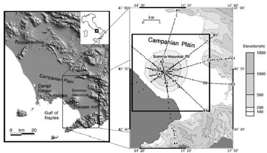
Regional location map (left) showing features cited in the text. Topographic map (right) of the Somma–Vesuvius region showing the Tomoves 1994 (line S) and 1996 (lines A–D) seismic reflection profile stations (solid circles) and shotpoints (A1, A2, etc.). The limits of the 3-D model are indicated by heavy black lines. GC: Gran Cono crater; TW: Trecase well.
The determination of basic parameters of seismic events such as absolute hypocentre locations and source mechanisms requires an accurate and realistic velocity model. In regions with irregular surface topography and strong lateral variation of near-surface velocities, large location errors can be introduced by the use of simple 1-D layered media for earthquake location. For most tectonically active regions, and for volcanoes in particular, the geological structures are complex and can only be represented by fully 3-D velocity models.
This is the case for the Vesuvius region. Prior knowledge (Finetti & Morelli 1974; Cassano & La Torre 1987; Zollo et al. 1996; Bruno et al. 1998; De Matteis et al. 2000) of the structure around Somma–Vesuvius (Fig. 2) includes:
- (1)
the Somma–Vesuvius volcanic edifice, consisting of volcanic products including lavas and pumice layers and probable structural complexity due to magma conduits and faulting during caldera formation;
- (2)
volcanic and sedimentary deposits covering the Campanian plain; and
- (3)
a Mesozoic carbonate basement that crops out around the Campanian plain and that is inferred to dip gently underneath this plain and to lie at about 2 km depth under the volcanic edifice.
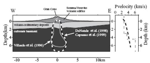
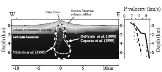
(Left) W–E cross-section through Somma–Vesuvius showing a schematic representation of the main structural features and the approximate zones of higher hypocentre density from Vilardo et al. (1996) (short-dashed line), and from De Natale et al. (1998) and Capuano et al. (1999) (long-dashed line). For all of these studies most of the hypocentres have depths greater than 2–3 km. (Right) Approximate P-velocity profile under Gran Cono from Vilardo et al. (1996) (short-dashed line), and De Natale et al. (1998) and Capuano et al. (1999) (long- dashed line).
The seismic activity at Mt Vesuvius is routinely monitored using standard location tools (hypo71, Lee & Lahr 1975, and Hypoinverse, Klein 1989) and assuming a flat-layered medium to represent the volcano structure. However, the use of a 1-D layered model and station corrections in the Vesuvius area is insufficient for several reasons.
First, a plane-layered model cannot adequately represent the shallow cover of low-velocity volcanic and sedimentary deposits that are concentric to and follow the volcano topography. The use of a 1-D model with a thick, constant-velocity upper layer approximating this structure results in an unreasonably high velocity for the low-lying regions around the volcano edifice and unreasonably low velocity for the interior of the edifice. This introduces significant velocity model errors along the event–station ray paths, which in turn lead to a significant reduction in the estimated depths of events under the volcano, as we show below. It is not appropriate to use station corrections to compensate for such path errors because the events of interest are in a volume of large size relative to the station–event distances and thus the ray paths to each station are not the same for all events.
A second limitation of 1-D layered models is their inability to represent accurately the known, significant variations in depth of the Mesozoic carbonate basement surface. The strong velocity jump from about 4 to about 6 km s−1 across this boundary controls the first-arriving wave types and ray paths between the events and stations, and consequently has a dominant effect on the event depth determinations.
Recently, refined 1-D and 2-D images of the shallow (up to 3–4 km depth) velocity structure of Mt Vesuvius and the Campanian Plain have been inferred from the Tomoves active seismic experiments performed in the area during 1994–1997 (Zollo et al. 1996, 1998, 2000, 2001; Gasparini 1998; De Matteis et al. 2000; ). Starting from the results of these studies, we have developed a 3-D velocity model for earthquake location by interpolation of the 2-D velocity sections obtained from tomographic inversion of the Tomoves data. Because this 3-D model is constructed independently of earthquake locations and earthquake traveltimes, it may be proposed that this model will give more accurate absolute locations than models based solely on earthquake data. There is also a need for this 3-D interpolated model as a reliable reference model for future fully 3-D tomographic inversions of the Tomoves data.
In the following, we begin with a summary of previous seismicity studies and of the geological setting and eruptive history of Somma–Vesuvius. We describe the methodology used to construct the new 3-D model, compare the predicted traveltimes in this model with arrival time picks from the Tomoves data set, and relocate natural seismic events under Vesuvius in this 3-D model and in a representative layered model. We compare and discuss these location results with regards to solution quality, station residuals, the VP/VS ratio, event depths and the P- and T-axes from first-motion source mechanisms.
Seismic Monitoring and Previous Seismicity Studies
The first three-component seismic station at Mt Vesuvius, OVO, was installed in 1971 (Fig. 1). By the early 1980s the permanent network at Mt Vesuvius consisted of the OVO station plus nine vertical-component, analogue stations located on the volcano edifice and on the surrounding plain. Seismic signals from remote stations are radio-transmitted to a surveillance centre in Naples, A/D converted at 100 Hz sampling frequency using the IASPEI software (Lee 1989) and then stored in SUDS format. Since 1987, portable, digital three-component stations, equipped with 3C sensors (Mark L4-3D) with local recording and 125 Hz sampling rate, have been deployed on the volcano to improve the station coverage during periods of high seismicity. Since 1996, five of these digital stations have been permanently deployed on the volcano. All stations are equipped with short-period seismometers with a natural frequency of 1 Hz.
Vilardo et al. (1996) presented probabilistic locations for Vesuvius events using a 1-D model (Fig. 2) consisting of an upper layer to about 3 km depth below sea level (bsl) with VP = 2.7 km s−1, a second layer to about 4.5 km depth with VP = 3.5 km s−1 and a basal half-space with VP = 6 km s−1; they used VP/VS ratios of 1.71–1.75. Their locations for 172 events from the period 1972–1994 (Fig. 2) show a maximum event density along the vertical axis through the Gran Cono crater axis, between about 3 and 6 km depth bsl, with a secondary peak between about 0 and 2.5 km depth. Vilardo et al. (1996) also obtained probabilistic focal mechanism solutions for 11 events using P and S polarizations. They found mainly strike-slip mechanisms with two conjugate orientations for the P- and T-axes: N–S P-axes with E–W T-axes, and E–W P-axes with N–S T-axes.
De Natale et al. (1998) and Capuano et al. (1999) examined 3-D earthquake locations in a smooth 3-D model (De Natale et al. 1998) for Vesuvius obtained from inversion of earthquake traveltimes using the SIMULPS linearized inversion program (Thurber 1983; Evans et al. 1994). This model contains a broad high-velocity zone along the Gran Cono crater axis and has a maximum P velocity of about 4.5 km s−1 at 6 km depth bsl (Fig. 2). This model lacks a distinct carbonate basement, which would be represented by VP > 5 km s−1. A VP/VS ratio of 1.76 is used to calculate S traveltimes. The resulting seismic event locations for 155 events from the period 1987–1995 (Fig. 2) are concentrated along the crater axis near the axial high-velocity zone, at depths from 0 to more than 7 km. Most events fall in the depth range 2–6 km, with a secondary cluster of events near 0.5 km depth. Capuano et al. (1999) performed probabilistic P and S polarization mechanism determinations for 15 of these events. They found predominantly strike-slip mechanisms but no clear pattern in the orientation of P- and T-axes.
Geological setting and eruptive history of somma–vesuvius
Somma–Vesuvius is a composite volcanic complex formed by an older volcano, Mt Somma, and a young crater, Mt Vesuvius. This structure is part of a volcanic field (Fig. 1) that is located in a graben-like structure bordered by Mesozoic carbonate rocks. The volcanic field includes the Campi Flegrei caldera and the Roccamonfina stratovolcano. The graben developed in Pleistocene times and was filled by marine and fluvial sediments interlayered with volcanic products. Volcanic activity in the Bay of Naples started about 120 kyr ago (Arnò. 1987). A major ignimbrite eruption occurred 35–39 kyr BP giving rise to a thick deposit (Campanian Ignimbrite) that extends throughout the Campanian Plain.
The Somma–Vesuvius edifice is built entirely on the Campanian ignimbrite and is therefore younger than 35 kyr. During the past 20 kyr, seven Plinian eruptions have occurred at intervals of some thousands of years. The last one occurred in 79 AD. Each Plinian eruption produced between 5 and 11 km3 of pyroclastic rocks that devastated an area of 20–30 000 hectares. The present summit caldera (Mt Somma) was formed as a consequence of these eruptions. Although Mt Vesuvius activity in late Roman times and in the Middle Ages is not well documented, available information indicates a major explosive eruption in 472 AD and less violent eruptions around 511 and 1139 AD. Vesuvius then seems to have been dormant until 1631 AD, when it erupted violently. From 1631 to 1944 it was in almost continuous Strombolian activity. During this interval it produced mostly leucite tephritic lavas that cap the SSE sector of the volcano edifice. Since 1944 Vesuvius has exhibited moderate, low-magnitude seismicity (Md ≤ 3.6) and no significant volcanic activity except for fumaroles in the Gran Cono crater area (Bonasia et al. 1985; Zollo et al. 2001).
Important information on the shallow structure of the volcano comes from a deep borehole drilled by the AGIP petroleum company at Trecase on the SE slope of Somma–Vesuvius. This hole penetrated the whole volcanic sequence and reached the Mesozoic carbonate basement rocks at a depth of 1.665 km bsl (Principe et al. 1987). The depth and shape of the Mesozoic carbonate basement surface beneath Mt Vesuvius has been inferred from Bouguer anomalies calibrated with offshore seismic reflection data (Finetti & Morelli 1974) and Trecase borehole data. Bruno et al. (1998) have mapped the limestone top around Mt Vesuvius using migrated reflection data from AGIP.
Recently, 2-D sections of the shallow velocity structure (up to 3–4 km depth) of Somma–Vesuvius and the Campanian Plain have been obtained from the Tomoves active seismic refraction experiments performed in the area during 1994–1997 (Zollo et al. 1996, 1998, 2000, 2001; Gasparini et al. 1998; De Matteis et al. 2000). These 2-D sections show P velocities in the range 1.7–5.8 km s−1 and give an image of the top of the Mesozoic carbonate basement rocks. The basement surface generally dips from the edges of the Campanian Plain towards the volcano, consistent with the Bouguer anomaly pattern (Cassano & La Torre 1987; Berrino et al. 1998), and this surface appears to be continuous underneath the volcano. A prominent feature is an 8 km wide depression of the carbonate top of about 1 km depth. This depression is located under the north side of the volcano with a southern limit beneath the Mt Somma caldera; it is well resolved by the tomographic inversions.
A shallow high-velocity body under the Mt Somma caldera is indicated by both first- and reflected P-wave arrivals. This high-velocity body, which overlies the Mesozoic carbonates underneath the summit caldera, may be associated with a palaeovolcanic or subvolcanic (solidified dykes) structure. The range of inferred velocities is consistent with in situ and laboratory measurements of solidified lavas (Zamora et al. 1994; Bernard 1999).
A 3-D velocity model for vesuvius
We construct a 24 × 24 × 9 km, 3-D P-wave velocity model for Somma–Vesuvius and surroundings by interpolation of the smooth, 2-D velocity sections (Zollo et al. 2000, 2001) obtained by inversion of the Tomoves 1994 and 1996 seismic refraction profiles. The seismic profiles and corresponding 2-D velocity sections have a radial distribution around Somma–Vesuvius, centred near the peak of Gran Cono (Fig. 1). Because this geometry aligns with the approximately cylindrically symmetric topography of Somma–Vesuvius, we chose to interpolate between the 2-D sections along circumferences at constant depth, centred on the crossing point of the profiles (hereafter referred to as circumferential interpolation).
Interpolation procedure
The circumferential interpolation procedure is described in detail in the Appendix and summarized here. We use linear interpolation exclusively for all stages of constructing the 3-D model. To avoid strong oscillation or discontinuity in velocity near the crossing point of the profiles, the 3-D model is constrained to be smooth and approximately cylindrically symmetric within a few kilometres of the crossing point.
The 2-D Tomoves velocity sections present a fairly complete image of the velocity structure of the volcanic edifice and surrounding volcano-sedimentary deposits. However, because the first-arriving signals that penetrate the carbonate basement are diffracted head waves, only the top of the carbonate basement is sampled. Consequently, the 2-D velocity sections have no resolution below depths of about 1–5 km. Thus a primary concern in the construction of the 3-D model is the identification of the depth to the carbonate basement along each 2-D section and the extrapolation of this structure throughout the 3-D model.
We use a three-stage procedure to construct the 3-D velocity model (Fig. A1). First, a depth contour for the carbonate basement top is determined along each of the 2-D velocity sections. Second, a surface that represents the carbonate basement for the 3-D model region (Fig. 3) is obtained by circumferential interpolation of the basement depth contours from each 2-D section. A constant-gradient velocity profile of 5.5 + 0.2 (depth − 1.0 km) km s−1 is assigned to all nodes of the 3-D model lying below this surface. Finally, the part of the 3-D model above the basement surface (the volcano-sedimentary cover and Somma–Vesuvius edifice) is formed by circumferential interpolation of the velocity on each 2-D section intersected by the relevant circumference. A minimum velocity value of 1.7 km s−1 is allowed at any node.
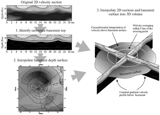
Schematic diagram of the circumferential interpolation procedure.
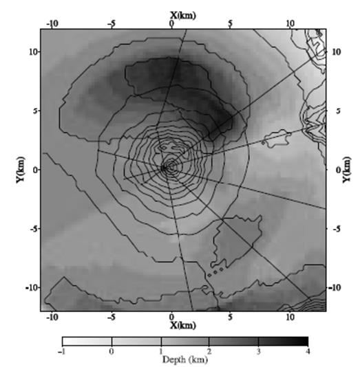
Contour map of the carbonate basement surface in the 3-D model obtained by circumferential interpolation of the basement depth determined for each 2-D velocity section.
This procedure produces a 3-D model (Fig. 4) that (1) is compatible with the observed Tomoves seismic profile traveltimes, (2) has a smooth, well-defined carbonate basement surface, and (3) avoids artefacts due to the limited depth resolution of the 2-D sections. However, there is some mixing of higher ‘carbonate’ velocities and lower ‘volcano-sedimentary’ velocities at locations in the 3-D model for which the corresponding interpolation circumference intersects adjacent 2-D sections at points alternately above and below the basement surface. In addition, because the smooth 2-D sections only represent a continuous transition in velocity between the ‘volcano-sedimentary’ cover and the ‘carbonate’ basement, excessively high velocities (> 4 km s−1) for some of the deeper parts of the ‘volcano-sedimentary’ cover are carried over to the 3-D model.
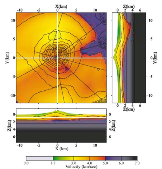
The interpolated 3-D model shown as a horizontal section at 1 km depth and vertical sections through Gran Cono viewed from the south and from the east.
The new 3-D model includes the depression to the north of Vesuvius (Fig. 3) and the shallow high-velocity body under the volcano (Fig. 4) identified in earlier work and in the Tomoves 2-D sections. However, due to the smoothing around the crossing point of the 2-D profiles, the high-velocity structure under the volcano is reduced to a broad, dome-shaped feature in the volcano-sedimentary layer.
Verification of the 3-D velocity model
We assess the quality of the 3-D interpolated velocity model by examining the consistency between the observed and calculated traveltimes for the in-profile shot gathers (shots and stations on the same profile) and fan shot gathers (shots on one profile and recording stations on a crossing profile) (cf.Fig. 1). The traveltimes are computing using a method valid for a 3-D heterogeneous medium based on the finite difference solution of the eikonal equation (Podvin & Lecomte 1991); this same method is used below for 3-D earthquake location. Note that because the calculated traveltimes are obtained with a fully 3-D model, geometry and eikonal solution, they can be compared directly with the observed times.
Only the along-profile shot data were used to construct the 2-D tomographic lines and consequently the 3-D interpolated model. Thus the comparison of in-profile arrival time curves serves as a check on the interpolation algorithms, whereas the comparison of fan arrival time curves gives an assessment of the general reliability of the new 3-D model in generating traveltimes.
As expected, for the along-profile shots, most of the calculated times fall within the uncertainty range of the observed times or just outside this range, typically with an error of ≤0.2 s (Fig. 5). The most significant mismatch is found along profile A, where the calculated times for paths passing through the volcano from shot A2 are late, while those for shot A3 are early at offsets of 5–8 km from the shotpoints. The good agreement for the changes in apparent velocity at around 2–3 km offset and for the times at long offsets for shots D2 and C4 justify the choice of 5.0 km s−1 for the cut-off velocity for determination of the carbonate basement depth. This agreement also supports the choice of constant gradient velocity profile below the basement depth, although only the velocity profile just below the basement is well constrained by the shot data.
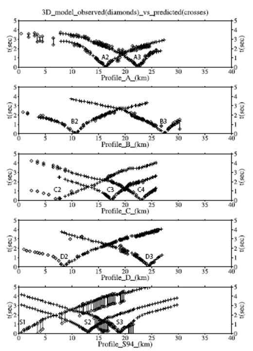
A comparison of observed arrival times from the Tomoves along-profile shot data (diamond symbols with a bar between the earliest and latest possible times for the first arrival) and the corresponding predicted first-arriving P times from the 3-D interpolated model (cross symbols). The horizontal axis shows the straight line distance in kilometres to each recording station from the first shot on each profile (i.e. shots A1, B1, C1, D1 and S1). Predicted times are only shown for shots and stations that lie within the bounds of the 3-D model.
The calculated times for the fan shot gathers fall within the uncertainty range of the observed times or just outside this range, typically with an error of ≤0.2 s (Fig. 6). The predicted arrival times are systematically lower along the central parts of fans C4A, B3D and D3B; this could be due to an overestimate in velocity in the 3-D model under and to the west of the Gran Cono. The very good agreement between observed and predicted times at wide-angle offsets for all of the fan gathers shows that the 3-D model produces accurate traveltimes for rays passing through the deeper parts of the ‘volcano-sedimentary’ layer and the top of the carbonate basement.
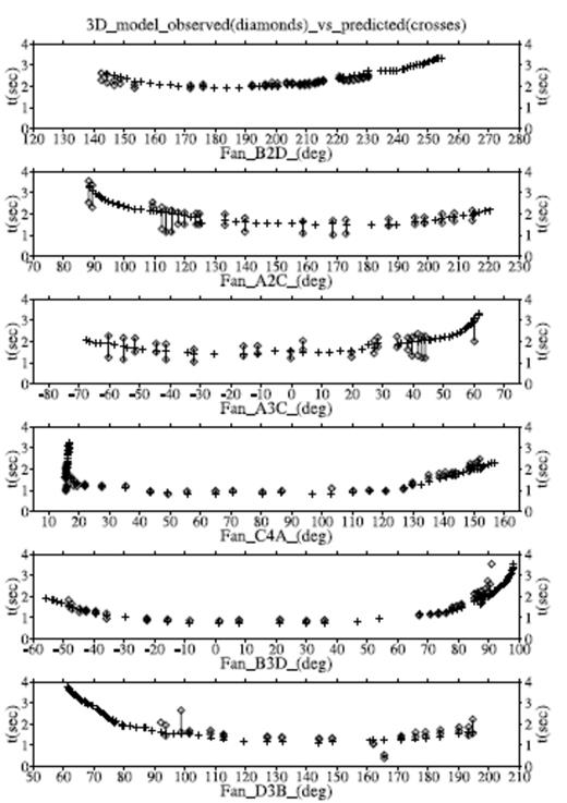
A comparison of observed arrival times from the Tomoves fan shot data (diamond symbols with a bar between the earliest and latest possible times for the first arrival) and the corresponding predicted first-arriving P times from the 3-D interpolated model (cross symbols). Fan data are denoted by a letter and number indicating the shotpoint followed by a single letter indicating the recording line. The horizontal axis gives the azimuth from the shotpoint to the recording stations in degrees east of north. Predicted times are only shown for shots and stations that lie within the bounds of the 3-D model.
From these comparisons we may conclude that the interpolated 3-D model is highly consistent with the observed P arrival times and that the absolute values of the errors in predicted arrival times are < 0.2 s in the central part of the model. We will use the 1σ value of 0.1 s for representing the normal error in predicted traveltimes in the earthquake location procedure.
Construction of a representative layered model
To help in judging the utility of the interpolated 3-D model for earthquake location, we have constructed a simple 1-D layered model that best fits the observed P arrival times derived from the Tomoves shots. However, it is not possible to construct a 1-D model that fits the traveltimes as well as the 3-D model. This difficulty arises in part because the observed arrival time data require an increase in velocity with depth in the shallow subsurface following the volcano topography. This structure cannot be represented by a velocity gradient in a 1-D upper layer because this leads to very low velocities near the top of the volcano, and relatively high velocities at the surface in the volcano-sedimentary deposits on the surrounding Campanian plain. Similarly, we cannot represent an irregular carbonate basement surface with a 1-D model, although active seismic data and prior geological information require such a surface.
To determine a best-fitting layered model we use a trial-and-error approach. This approach is easy to implement for this simple problem and it gives direct insight into the limitations of 1-D models for fitting the data. We find that a 1-D model with one layer (VP = 3.0 km s−1 to a depth of 2.0 km bsl) over a half-space (VP = 6 km s−1) gives a satisfactory fit to the observed traveltimes. Fig. 7 shows a comparison of the calculated and observed arrival times for in-profiles shot gathers using the 1-D model. Typically the calculated arrival times fall within about 0.5 s of the observed times. However, there are some more significant mismatches (around 1 s) at near offsets along profile A (early predicted arrivals) and along profile C (early and late predicted arrivals).
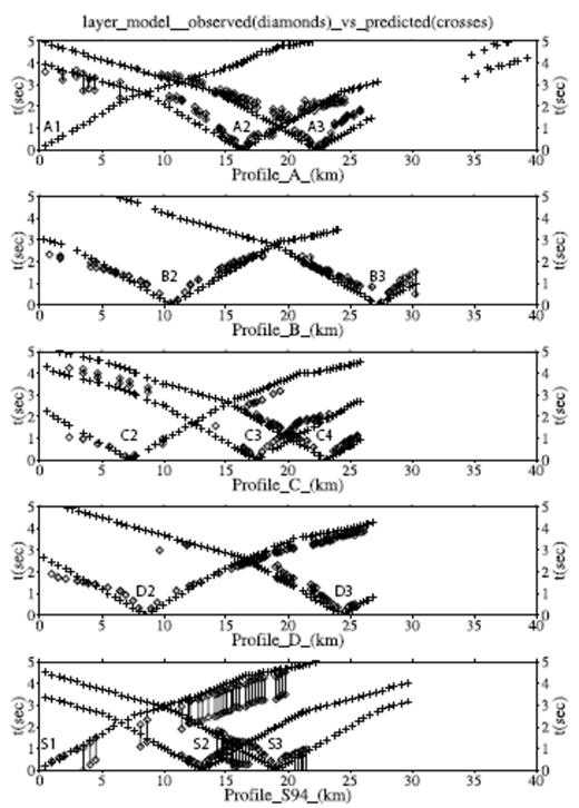
A comparison of observed arrival times from the Tomoves along-profile shot data (diamond symbols with a bar between the earliest and latest possible times for the first arrival) and the corresponding predicted first-arriving P times from the representative 1-D layered model (cross symbols). The horizontal axis shows distance in kilometres from the first shot on each profile (i.e. shots A1, B1, C1, D1 and S1).
Global search earthquake locations for vesuvius
We have obtained probabilistic earthquake locations for Mt Vesuvius earthquakes using a non-linear, global search method. Unlike linear approaches, global search methods can be easily applied with 3-D velocity models because they do not require partial derivative information, which is difficult or impossible to obtain in complex models. In addition, a probabilistic earthquake location, represented by a posterior probability density function (PDF) of model parameters, produces comprehensive uncertainty and resolution information and allows for the detection of multiple ‘optimal’ solutions (Tarantola & Valette 1982; Lomax et al. 2000).
Earthquake location methodology
For the non-linear global search locations in this paper, we use a software package called NonLinLoc (Lomax et al. 2000; available on the Internet at the ORFEUS Seismological Software Library: ).
The NonLinLoc location algorithms follow the probabilistic formulation of inversion presented in Tarantola & Valette (1982) and Tarantola (1987) and the equivalent methodology for earthquake location (i.e. Tarantola & Valette 1982; Moser et al. 1992; Wittlinger et al. 1993; Lomax et al. 2000). The unknown parameters for an earthquake location are the hypocentral coordinates x = (x, y, z) and the origin time T; the observed data are a set of arrival times, t, and a theoretical relation gives predicted traveltimes, h. Tarantola & Valette (1982) showed that if the theoretical relationship and the observed arrival times are assumed to have Gaussian uncertainties with covariance matrices CT and Ct, respectively, and if the prior information on the origin time parameter T is taken as uniform, then it is possible to integrate the PDF over T to obtain the marginal PDF for the spatial location parameters, σ(x). This marginal PDF reduces to (Tarantola & Valette 1982; Moser et al. 1992)
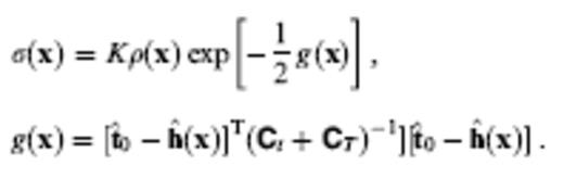
In this expression K is a normalization factor, ρ(x) is a density function of prior information on the model parameters, and g(x) is an L2 misfit function. t^0 is the vector of observed arrival times t minus their weighted mean, and h^ is the vector of theoretical traveltimes h minus their weighted mean, where the weights wi are given by
NonLinLoc has two different search algorithms to obtain an estimate of the location PDF (eq. 1). The first is a grid search consisting of a sequence of successively finer nested grid searches within a spatial x, y, z volume. The grid search is very time-consuming but performs a systematic, exhaustive coverage of the search region and thus can identify multiple optimal solutions and highly irregular confidence volumes.
The second search algorithm is a Metropolis–Gibbs sampler that is similar to algorithms described in Sen & Stoffa (1995) and Mosegaard & Tarantola (1995), with the addition of three distinct sampling stages to obtain adaptively an optimal step size for the walk. The Metropolis–Gibbs sampler consists of a directed walk in the solution space (x, y, z), which tends towards regions of high likelihood for the location PDF, σ(x), given by eq. (1). At each step, the current walk location, xcurr, is perturbed by a vector, dx, of arbitrary direction and given length l to give a new location, xnew. The likelihood σ(xnew) is calculated for the new location and compared to the likelihood σ(xcurr) at the current location. If σ(xnew) ≥ σ(xcurr), then the new location is accepted. If σ(xnew) < σ(xcurr), then the new location is accepted with probability P = σ(xnew)/σ(xcurr). When a new location is accepted it becomes the current location and may be saved as a sample of the location PDF.
The Metropolis–Gibbs sampler performs well with moderately irregular (non-ellipsoidal) PDFs with a single optimum solution, but because it is a stochastic search it may give inconsistent recovery of very irregular PDFs with multiple optimal solutions. The Metropolis–Gibbs sampler is only moderately slower (about 10 times slower) than linearized, iterative location techniques, and is much faster (about a hundred times faster) than the grid search. (see Lomax et al. 2000 for more details)
To make the location program efficient for complicated 3-D models, the traveltimes between each station and all nodes of an x, y, z spatial grid are calculated once using a 3-D version (Le Meur 1994; Le Meur et al. 1997) of the Eikonal finite difference scheme of Podvin & Lecomte (1991) and then stored on disk as traveltime grid files. This storage technique was used by Wittlinger et al. (1993) and in related approaches by Nelson & Vidale (1990) and Shearer (1997). The forward calculation during location reduces to retrieving the traveltimes from the grid files and forming the misfit function g(x) in eq. (1). After the traveltimes are calculated throughout the grid, the gradients of traveltime at each node are examined to generate a grid of take-off angles for the ray from a source at each grid node to the station. These take-off angles are used for fault plane solution estimations.
A grid of PDF values obtained by the grid search, samples drawn from this grid, or samples of the PDF obtained by the Metropolis–Gibbs sampler represent the complete probabilistic spatial solution of the earthquake location problem. This solution indicates the uncertainty in the spatial location due to Gaussian picking and traveltime calculation errors, the network–event geometry and the incompatibility of the picks. The location uncertainty will in general be non-ellipsoidal (non-Gaussian) because the forward calculation involves a non-linear relationship between hypocentre location and traveltimes.
In this study, the maximum-likelihood (or minimum-misfit) point of the complete, non-linear location PDF is selected as an ‘optimal’ hypocentre. The maximum likelihood hypocentre location is used for the determination of ray take-off angles and phase residuals. ‘Traditional’ Gaussian or normal estimators such as the expectation E(x) and covariance matrix C are obtained from the gridded values of the normalized location PDF or from samples of this function (e.g. Tarantola & Valette 1982; Sen & Stoffa 1995). The 68 per cent confidence ellipsoid is obtained from singular value decomposition (SVD) of the covariance matrix C.
2013 Location results for Somma–Vesuvius
Earthquake locations in the 3-D and 1-D models were performed using P and S phase picks from about 400 local earthquakes under Somma–Vesuvius in the period 1989–1998. We only use S picks coming from horizontal-component records, and locate only those events for which six or more P and S observations and at least two S observations were available. We applied the NonLinLoc Metropolis–Gibbs search method (described above) within the volume covered by the 3-D model, with 10000 accepted samples and 1000 saved samples to represent the non-linear location PDF.
The Tomoves refraction experiments give information about the P-velocity structure around Vesuvius. The earthquake locations, however, are strongly dependent on the VP/VS ratio. Below, we present results for a typical VP/VS ratio of 1.76, used by De Natale et al. (1998) and others, and for a relatively high VP/VS ratio of 1.90, which produces better location results and smaller residuals for the 3-D model.
For the calculation of average station residuals, we use the maximum likelihood locations for all events with a minimum of 10 phase readings and a maximum azimuth gap of 120°. For the analysis and plotting of hypocentres, we use the maximum likelihood locations with a maximum 68 per cent confidence ellipsoid semi-axis length of 1.0 km, a maximum rms error of 0.1 s and a maximum azimuth gap of 120°. Table 1 summarizes the number of high-quality hypocentres available after this selection by ellipsoid semi-axis length, the rms error and the azimuth gap. It should be noted that the number of selected and plotted events is different for each model type and VP/VS ratio, and that a larger number of events are used for the residual calculations than for the hypocentre plots.

Number of events with axis <1.0 km, rms <0.1 s and gap< 120°.
The locations with both the layered and the 3-D model assuming VP/VS = 1.76 produce average P and S station residuals that are mostly negative near the middle of the volcano edifice and mostly positive around the base of the volcano (Figs 8a, b, e and f). This pattern is an indication of an inadequate VP/VS ratio for the volcano edifice. Indeed, using VP/VS = 1.90 we find smaller residuals in general and a more heterogeneous spatial mix of residual polarities over the volcano edifice (Figs 8 c, d and g), except for the layered model S residuals (Fig. 8h). The P residuals found with VP/VS = 1.90 are slightly larger in magnitude for the 3-D model than for the layered model at the top of the volcanic edifice, but both the P and the S residuals for the 3-D model are mostly much smaller around and away from the volcano. In particular, the small P residuals for the 3-D model at more distant stations SCI, NL9 and VIS and the small S residual at station VIS indicate that the 3-D model represents well the lateral topographic and structural variations moving from the volcanic edifice to the surrounding sedimentary plain (SCI) and into the carbonate mountains (NL9 and VIS). This result is important because the correct modelling of the traveltimes and ray paths to the more distant stations is critical for constraining the event depths and focal mechanisms.


(a)–(d) Average P station residuals for VP/VS = 1.76 for (a) the 3-D model and (b) the layered model, and for VP/VS = 1.90 for (c) the 3-D model and (d) the layered model. (e)– (h) Average S station residuals for VP/VS = 1.76 for (e) the 3-D model and (f) the layered model, and for VP/VS = 1.90 for (g) the 3-D model and (h) the layered model
Relatively large, negative P residuals at stations near the top of the volcano are inferred using the 3-D model. This result may indicate that the velocities in this model are too low in the middle of the volcanic edifice somewhere above the earthquake hypocentres. This assertion contradicts the proposition of a possible overestimate of velocities in the volcano edifice invoked above to explain slightly early arrivals on fan shot gathers. However, since the 2-D tomographic sections were not constrained to agree at the crossing point of the refraction lines, and consequently the 3-D model was constructed with a relatively strong lateral smoothing under the volcanic edifice, it will be necessary to re-examine this issue when a more detailed 3-D model obtained from fully 3-D inversion of the shot data is available. Also, we note that the anomalous large average station residual estimates for CRT were obtained from only two P arrival times.
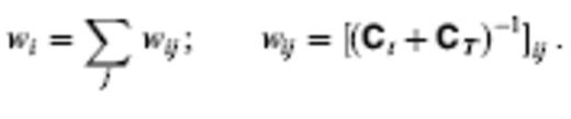
The layered model locations for both VP/VS ratios show a main cluster of events at just above 2 km depth and a scattering of events at greater depth (Figs 9 and 10). Although the main cluster of events is concentrated, it is positioned just above the sharp layer interface (3–6 km s−1) where ray paths and the location misfit function are discontinuous. Thus, the presence of a tight cluster of locations near this boundary is most probably due to a biasing effect of the station, velocity model and ray geometries, and probably does not reflect the true absolute event locations.
Location results for VP/VS = 1.76 showing maximum likelihood locations for (a) the 3-D model and (b) the layered model.
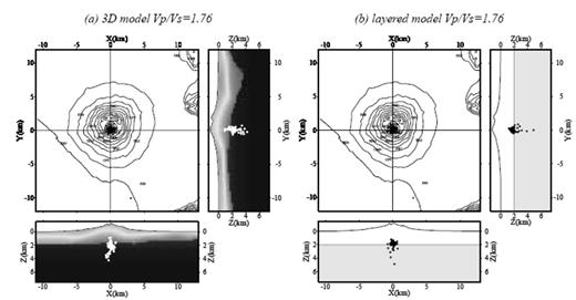
Location results for VP/VS = 1.90 showing maximum likelihood locations for (a) the 3-D model and (b) the layered model.
The 3-D locations, in contrast, lie both above and below the interface in the 3-D model marking the carbonate basement at about 1.75 km depth under Gran Cono (cf.Fig. 3) and do not show tight clustering (Figs 9 and 10). Thus, we expect that there is not a significant biasing effect on the 3-D locations due to the basement velocity contrast. This result, the good agreement between the observed and calculated traveltimes for the Tomoves shots in the 3-D model and the large number of high-quality locations and relatively small station residuals for the 3-D locations with VP/VS = 1.90 allow us to conclude that the 3-D locations with VP/VS = 1.90 give the best representation of the true absolute event locations.
Fault plane solutions
We estimate the focal mechanisms and corresponding compression (P) and tension (T) axes from P-wave first-motion polarities for a subset of the 1989–1998 events underneath Mt Vesuvius using the grid search mechanism determination algorithm FPFIT (Reasenberg & Oppenheimer 1985). For input to FPFIT we use the maximum-likelihood hypocentre and corresponding ray take-off angles for the 3-D model locations with VP/VS = 1.90 for 30 events with 10 or more first-motion observations. The presence in the data set of both positive and negative first motions for individual stations and of many different patterns of polarity relationships between stations for individual events indicate that a large variety of mechanisms are present (Fig. 11). However, the number of first-motion readings and their coverage of the focal sphere are not sufficient to give good constraint on the fault plane orientations for individual events. For these reasons we discuss here only the gross features of the distribution of P- and T-axes.
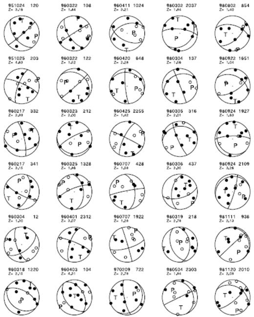
Lower-hemisphere projections of the 30 individual FPFIT mechanism determinations showing compressional (solid circles) and dilatational (open circles) first motions and P- and T-axes.
Fig. 12 shows the distribution of P- and T-axes for the preferred fault plane solutions obtained for the 30 events with 10 or more first-motion observations. Although there is a large variation in the orientation of the axes, Fig. 12 indicates a clustering around roughly N–S to near-vertical directions for the tension axes, and ESE–WNW to near-vertical directions for the compression axes. There is no clear pattern to the orientation of P- and T-axes at depth. For a better understanding of the focal mechanisms of events underneath Somma–Vesuvius, it may be necessary to investigate in more detail the larger events for which high signal-to-noise level waveforms and information from regional stations are available.
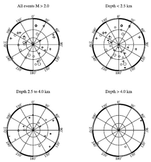
Stereographic views of pressure (crosses) and tension (circles) axes from 30 FPFIT first-motion mechanism determinations for events with magnitude M ≥ 2, events with depth h ≤ 2.5 km, events with depth 2.5 ≤ h ≤ 4.0 km and events with depth h > 4.0 km.
Discussion
We have developed a 3-D P-velocity model (Fig. 4) for Somma–Vesuvius volcano and surroundings using a three-stage interpolation procedure applied to 2-D velocity sections obtained by inversion of the Tomoves refraction profiles (Fig. 1). We construct this 3-D model so that it contains a carbonate basement surface (Fig. 3) that matches prior geological information, including the basement depth observation from the Trecase well. We confirm that the 3-D model gives predicted P arrival times for the Tomoves in-profile and fan shot gathers that match the observed times within 0.2 s (Figs 5 and 6). We use this new 3-D model and an optimal 1-D layered model to obtain non-linear global search earthquake locations of events under Vesuvius for the period 1989–1998.
We have examined location results assuming a typical VP/VS ratio of 1.76 but find that a relatively high VP/VS ratio of 1.90 produces better results and smaller average station residuals (Table 1, Fig. 8). Most of the stations used in this study are located on or near the Somma–Vesuvius volcanic edifice, thus the high VP/VS ratio may reflect properties of this structure such as extreme compositional heterogeneity and complexity, abundant microfracturing, or the presence of fluids. Since there are few stations and S readings available off the volcanic edifice, the results of this study do not exclude a more typical VP/VS ratio of ∼1.8 for the carbonate basement and surrounding carbonate outcrops. Locally high VP/VS ratios may be expected in volcanic structures; for example, Aster & Meyer (1988) found high VP/VS ratios of up to 2.20 in the central part of the nearby Campi Flegrei caldera.
We expect that a 1-D layered model cannot satisfy the prior information of the topographic and geological structure for the Somma–Vesuvius region, and indeed in this work we can only obtain an ‘optimal’ layered model that gives a relatively poor match to the observed Tomoves profile times (Fig. 7). For both VP/VS ratios, the event locations obtained using this 1-D model are of lower quality than those for the 3-D model, as indicated by the number of high-quality events recovered or by the distribution and size of average station residuals. The 1-D locations (Fig. 10a) show a tight clustering of events just above the sharp interface at 2 km bsl representing the carbonate basement; this clustering of events is most probably an artefact due to the strong effect of the interface on the misfit function and ray paths.
Most of the maximum-likelihood locations obtained with the 3-D model and the preferred VP/VS ratio of 1.90 are concentrated within about 1 km of the Gran Cono crater axis at depths of about 1–3.5 km bsl (Figs 10a and 13). This is significantly shallower than the 3–6 km depth range found by Vilardo et al. 1996) and the 2–6 km depth range reported by De Natale et al. (1998) and Capuano et al. (1999) for the main group of events (Fig. 13). This difference in event depths can be attributed to the higher VP/VS ratio and the presence of higher velocities at shallower depth in the 3-D model in this work than in the models in previous studies (Fig. 13). The results of all these earthquake location studies are strongly dependent on the velocity variations and positions of strong interfaces in the models. The depths obtained with the new 3-D model are probably most representative of the true absolute event depths because this model is derived from shot data with known source locations and origin times and because it includes a carbonate basement interface compatible with the Trecase well profile, shallow seismics and gravity data.
(Left) The maximum-likelihood locations (stars) from this work for VP/VS = 1.90 in the 3-D model compared with the approximate zones of higher event density from Vilardo et al. (1996) (short-dashed line), and from De Natale et al. (1998) and Capuano et al. (1999) (long-dashed line). For all of these previous studies most of the events have depths greater than 2–3 km. (Right) Approximate P-velocity profile under Gran Cono from Vilardo et al. (1996) (short-dashed line), De Natale et al. (1998) and Capuano et al. (1999) (long-dashed line), and this study (solid line).
Our first-motion mechanism determinations show a large variation in the orientation of compression and tension axes, but give a weak indication of a dominance of roughly N–S to near-vertical directions for the tension axes and ESE–WNW to near-vertical directions for the compression axes. It is not possible to give a definitive interpretation of these results. They may have some relation to the approximately NE–SW trend of regional faults near Vesuvius (Bruno et al. 1998) and to the orientation of basin or graben structures in the carbonate basement under the Campanian plain (cf.Fig. 3). However, the variety of mechanisms may also reflect stress variations and structural heterogeneity at a smaller scale within the volcanic edifice.
Russo et al. (1997) studied the mechanical stability of Mt Vesuvius volcano through axisymmetric, numerical, finite element modelling of the stress distribution inside and beneath the volcano edifice due to the combined effects of local and regional stress sources. They examined models that included a strong, flat, low-to-high rigidity contrast associated with the lithological transition between the shallow volcanic sediments and the Mesozoic carbonates. According to their simulations, a shear stress increase is expected around this structural discontinuity in response to symmetric tensional or strike-slip regional stress regimes. This effect is amplified near the crater axis due to the additional stress related to the topographic relief of the volcano edifice. The calculated orientations of principal stresses in this model would favour near-vertical, normal-fault earthquakes (horizontal T- and vertical P-axes), in contrast with the results of Vilardo et al. (1996) and the present study, which show dominantly horizontal P- and T-axes. The possible irregular, faulted shape of the carbonate surface discontinuity underneath the volcano complex could explain this discrepancy since the shear stress orientations near the discontinuity strongly depend on its morphology.
The event depths obtained in this work imply that the seismicity at Mt Vesuvius is mainly concentrated in the upper 2 km of the carbonate basement, while some events may locate just above the basement level at around 1.5 km depth (Fig. 13). This result suggests an important role played by the lithological transition between the volcanic sedimentary and Carbonate Mesozoic sequences in deformation and fracturing processes occurring inside and beneath Mt Vesuvius during the present quiescent phase of the volcano. The axial cone distribution of background seismicity at depths of 1–3.5 km bsl can be explained through the combined effects of shear stress increase around the zone where the largest change in rock rigidity is expected, i.e. the carbonate top discontinuity, and rock strength weakening due to the dense fracturing associated with magma ascent to the surface during the eruption episodes.
The new 3-D velocity model we have presented here contributes to the understanding of the shallow structure of Mt Somma–Vesuvius volcano, and it will improve the accuracy of earthquake location and depth estimates during the continuous monitoring of the volcano activity. In the future, higher-quality locations and more reliable mechanisms for a limited set of earthquakes under Somma–Vesuvis can be obtained by careful selection and analysis of the waveforms for events recorded on high signal-to-noise, three-component digital instruments. Such a data set would also be useful to verify the relatively high VP/VS ratio obtained in this study. The 3-D model for the Somma–Vesuvius region can be improved when a fully 3-D inversion of the Tomoves along-profile and fan recordings becomes available. The development of such a 3-D model might include simultaneous inversion of the crossing profile data, a priori incorporation in the model parametrization of a carbonate basement discontinuity surface, and use of the AGIP migrated reflection data (Bruno et al. 1998). The 3-D velocity model developed in this study provides an initial reference model for a fully 3-D tomographic inversion of the Tomoves data.
Acknowledgments
We thank A. Herrero, L. D'Auria, G. Russo, M. R. Frattini, M. Simini, G. Giberti, G. Iannaccone, G. De Natale and members of the Tomoves Working Group for discussions and assistance that contributed greatly to this work. This research was supported by the European Union project ENV4-4980696 (TOMOVES). Publication number 374, UMR Géosciences-Azur-CNRS-UNSA.
Appendix
Appendix A: Circumferential interpolation procedure
We construct a 24 × 24 × 9 km 3-D P-wave velocity model for Somma–Vesuvius and surroundings by linear interpolation of velocity between the Tomoves 2-D velocity sections. This interpolation is performed along circumferences at constant depth (Fig. A1) and is referred to here as circumferential interpolation. The circumferences are centred on the crossing point of the 2-D profiles, and thus follow the approximately cylindrically symmetric topography of Somma–Vesuvius. The velocity at a point along a circumference in the 3-D model is interpolated from the velocity values at the points of intersection of the circumference with the two adjacent 2-D velocity sections.
We experimented with both cubic spline and linear interpolation. We find that with cubic splines the artefacts introduced by oscillations dominate over any advantage of the additional smoothness in comparison to linear interpolation, and thus we use linear interpolation exclusively for all stages of constructing the 3-D model.
The 2-D Tomoves velocity sections present a fairly complete image of the velocity structure of the volcanic edifice and surrounding volcano-sedimentary deposits. However, because the first-arriving signals that penetrate the carbonate basement are diffracted head waves, only the top of the carbonate basement is sampled, and thus the 2-D velocity sections typically have no resolution below depths ranging from about 1–5 km, depending on the section and the position on the section. In addition, because of the smooth parametrization used for the 2-D inversions, the carbonate basement depth is not identifiable on the 2-D sections as a sharp interface, but instead must be inferred by association with a given velocity contour. Thus it is important in the construction of the 3-D model to identify a depth to the carbonate basement along each 2-D section and to extrapolate this structure throughout the 3-D model.
We use a three-stage procedure to construct the 3-D velocity model (Fig. A1). First, a depth contour for the carbonate basement top is determined along each of the 2-D velocity sections. This is done by finding at each offset along the section the deepest point at which the velocity increases through 5.0 km s−1. If such a point does not exist, then the depth at which the velocity is maximal is taken as the basement depth. The cut-off value of 5.0 km s−1 is selected for determining the depth to the basement because this value lies between the expected velocity (De Matteis et al. 2000) for the basal part of the sediments (∼ 4 km s−1) and for the carbonate basement (∼ 6 km s−1), and because it produces a basement depth near the Trecase well close to the observed value of about 1.7 km bsl. Second, a surface that represents the carbonate basement for the 3-D model region (Fig. 3) is obtained by linear circumferential interpolation of the basement depth contours on each 2-D section. A constant-gradient velocity profile of 5.5+0.2 (depth − 1.0 km) km s−1 is assigned to all nodes of the 3-D model lying below this surface. This profile gives the best match to the large-offset observed times on the Tomoves shot data. Finally, the part of the 3-D model above the basement surface (the volcano-sedimentary cover and Somma–Vesuvius edifice) is formed by linear circumferential interpolation of the velocity at constant depth on each 2-D section intersected by the relevant circumference. A minimum velocity value of 1.7 km s−1 is allowed at any node. Bends in the 2-D velocity sections are treated correctly since the 2-D profiles are extrapolated into the 3-D model from their true positions in the 3-D model space.
To avoid strong oscillation or discontinuity in velocity near the crossing point of the profiles, the assigned velocity at points within 5 km of the crossing point is formed by a weighted average of (1) the circumferential interpolated velocity and (2) the mean of the velocity on all 2-D sections at the points where they intersect the corresponding circumference. The weight of the mean velocity contribution varies from 1 at the crossing point to 0 at 5 km radius, thus the 3-D model is forced to be smooth and approximately cylindrically symmetric within a few kilometres of the crossing point.
References
