


Summary
We present a method to model the propagation of surface waves in Cartesian structures showing isotropic and anisotropic 3-D heterogeneities. It is assumed that the background structure is laterally homogeneous and that the heterogeneities act as secondary sources, producing multiple scattering and coupling between the surface wave modes of the background structure. No far-field approximation is made, enabling in particular the heterogeneities to be located in the vicinity of the source or receiver. The heterogeneities may be strong and extended 3-D bodies or perturbations of layer boundaries.
Several applications are presented, including comparison to an exact solution for a cylindrical heterogeneity. The multiple-scattering series is shown to converge for strong heterogeneities of 10 per cent in S-wave velocity over several wavelengths. We analyse the influence of anisotropy and show in particular that some elastic coefficients, which are non-zero in mantle structures with crystals oriented in a non-horizontal flow, are able to distort the surface wave polarizations strongly.
1 Introduction
Classically, surface waves are used in seismology for determining the Earth's structure by inversion of their phase and group velocities, and for calculating source parameters by using phase and amplitude information. In most cases, very simple assumptions are made concerning wave propagation, and the effect of focusing or scattering by the 3-D nature of the Earth is not accounted for.
Although these assumptions are justified in most cases, some data present characteristic features that make it necessary to account for the complex effect of lateral heterogeneity. For example, Van der Lee (1998) observed important Rayleigh wave amplitude anomalies in North America that most probably arise from important near-source scattering. If not accounted for, this scattering will bias source parameter estimates. Laske et al. (1994) also showed that polarization anomalies of Rayleigh waves in the intermediate period range are more complex than in the long-period range. A careful analysis of their origin is necessary before they can be used, like the long-period ones, to improve the resolution of tomographic models.
These two examples illustrate the need to quantify the effect of different kinds of 3-D structures on surface wave propagation. They also indicate that a potential source of information lies in wavefield anomalies, which can become useful if appropriate data-analysis methods are developed.
The effect of 3-D isotropic and anisotropic heterogeneities on long-period surface waves has been studied in particular by Park & Yu (1992) using a free-oscillation formalism. For surface waves at shorter periods, that is mantle surface waves from 20 to 60 s period, crustal surface waves and surface waves in geotechnical applications, this formalism is not well-adapted, and formalisms based on surface wave modes in a Cartesian structure are better suited.
Surface wave propagation in Cartesian structures has been studied more in 2-D than in 3-D structures (see Kennett 1998, for a recent review). In 3-D structures, their scattering was first studied extensively by Snieder (1986). His formalism, based on Born scattering and the far-field approximation, is well-adapted to study the effect of small heterogeneities that are located far away from source and receiver, but not to study the effect of heterogeneities in the vicinity of a receiver, for example. A more complete method that can cope with the near-field and larger contrasts in the heterogeneities was developed by Bostock (1991) and Bostock & Kennett (1992). In this method, the model is composed of blocks, of possibly complex shapes, embedded in a reference layered structure. The fact that the structure inside each block must be laterally homogeneous in order to support a single set of local modes is the main limitation of this method. For complex 3-D structures, a large number of blocks have to be defined and their wavefields must interact with each other, leading to heavy computations.
A multiple forward scattering formalism was presented by Friederich et al. (1993). This method can handle general 3-D structures in a very effective way. Used in combination with an appropriate representation of the incoming wavefield, it provides a modern method for inverting teleseismic surface waves recorded at regional networks for the shear wave structure under the network (Friederich 1998).
In this paper, we present a very general scheme to synthesize surface waves propagating in 3-D Cartesian structures. It is based on multiple scattering and can handle 3-D isotropic and anisotropic structures embedded in a laterally homogeneous reference structure. It has a number of similarities with the multiple forward scattering method presented by Friederich et al. (1993). The main differences are that we focus on amplitude and polarization anomalies, and therefore keep multiple scattering in all directions. The mode coupling, especially between Rayleigh and Love waves, is emphasized and we allow for anisotropic heterogeneities. We show that our expressions satisfy the boundary conditions at tilted interfaces between layers. After a presentation of the theory, we compare the results of the method with those of an exact method in a geometrically simple situation. The limits of the method are then examined by using strongly heterogeneous isotropic structures. Finally, the specific features associated with propagation of surface waves in anisotropic 3-D structures are examined.
2 Theory
Our development is based on the same formulation as in Friederich et al. (1993): the structure is separated into a reference homogeneous structure and a heterogeneity superimposed on that structure; the wavefield is expressed as a sum of modes and we use the notion of potential field to describe the amplitude and phase of each mode in the horizontal plane. The main difference from Friederich et al. (1993) is in the way we handle multiple scattering. In addition, we also analyse the scattering due to anisotropic heterogeneities.
2.1 Usage of a reference Green's function
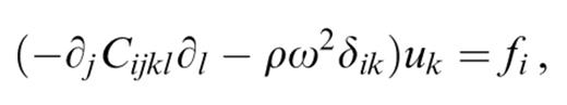
where u is the displacement, f the source function, ω the angular frequency, ρ the density and Cijkl the tensor of elastic coefficients. The associated boundary conditions are
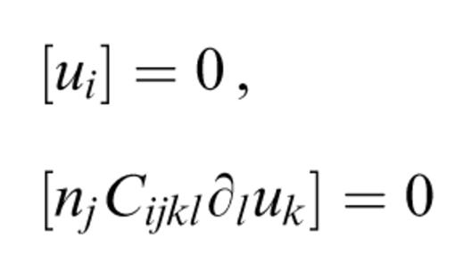
at each interface, where n is the normal to the interface and [] means a jump of the enclosed quantity over the interface. At the free surface, only the second of these two equations applies.
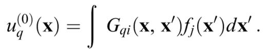
The solution is given in its general form by
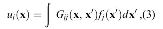
where Gij(x, x′) is a Green's function satisfying the same boundary conditions as u, and the integral is to be taken over the volume of the source.
Separating the structure into a laterally homogeneous reference structure and a perturbation, the elastic wave equation (1) can be written as
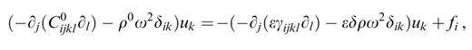
where the elements indexed 0 are related to the reference structure, whereas γijkl and δρ are the perturbations in elastic coefficients and density, respectively. We insert the parameter ε temporarily, in order to show explicitly which elements are related to the perturbation.
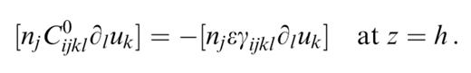
In addition to introducing heterogeneities in the layers, it can be desirable to displace the layer boundaries. Writing the boundary conditions in the perturbed model in a form suitable for using the Green's function in a reference structure is equivalent to introducing two discontinuities in traction in the reference model: one at the level h0 of the boundary in the reference structure,
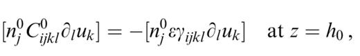
and one at the level h of the boundary in the perturbed model,
These traction discontinuities are equivalent to two sets of forces localized on the discontinuities,
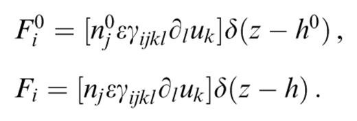
We can therefore replace the traction discontinuities by the forces F0 and F, which can be inserted in the source term. The differential equation on the left-hand side of eq. (4) is the equation of motion in the reference structure. Having inserted the forces F0 and F in the source term, the boundary conditions of the problem are also those of the reference structure (eqs 2). We can therefore write
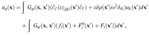
where Gqi(x, x′) is the Green's function in the reference structure. ∂j′ and ∂l′ denote derivatives with respect to x′j and x′l respectively.
In each region in between any two interfaces (one interface may be a layer boundary present in the reference structure and the other one in the perturbed model), the model parameters and the wavefield are continuous and have continuous derivatives. We can therefore apply Gauss's theorem in each of these regions to the first term on the right-hand side of eq. (8). This results in
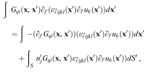
where S′ represents the region boundaries, i.e. the two interfaces, with normal n′ oriented outwards. A close examination of the boundary terms introduced by this application of Gauss's theorem reveals that they cancel the interface forces introduced to replace the traction discontinuities in eq. (7). The final equation for the displacement is therefore
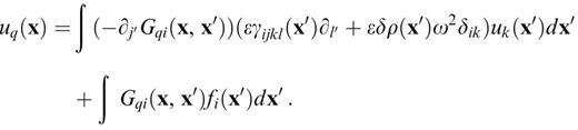
This equation satisfies the equation of motion and the boundary conditions in the perturbed model. Note that there are no interface terms other than those present in the volume integral, due to perturbations γijkl and δρ related to the displacements of the boundaries, and that we do not need to resort to a delta-function representation of the volume perturbation between old and new boundaries.
2 Multiple scattering
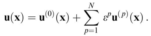
So far, no approximations have been made, but u(x) appears both on the left-hand side and on the right-hand side of eq. (10). In order to take advantage of the decomposition of the structure into a reference structure and a perturbation, we also separate the wavefield into a reference wavefield and a perturbation, expressed as a series in ε:
Inserting this into eq. (10), we obtain for each power of ε
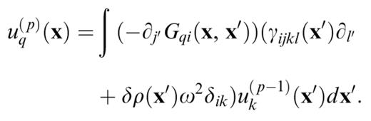
The order 0 term is simply the last term in eq. (10), that is, the wavefield generated by the source in the reference structure,
uq(p) is the scattered wavefield of order p. The obvious advantage of this formulation is that the Green's function has to be calculated only in the reference structure. The basic assumption is that the nature of the problem is such that the series converges. We note that eq. (10) is a Fredholm integral equation of the second kind. This kind of equation is well behaved and usually well suited to a solution in the form of a series (Hackbusch 1995). Keeping only uq(1) produces the classical Born approximation. In the development presented in this paper, we have kept several orders of scattering and verified the convergence of the series by checking in each case that the wavefield does not change significantly when adding a new term.
2.3 Modal decomposition and definition of potential
For surface waves in laterally homogeneous structures, the Green's function can be written as a sum of modes that propagate independently from each other. These modes are able to represent the wavefield that is trapped in the structure, but not the body waves that propagate at a steep angle and are not trapped. Lateral heterogeneities may convert energy from surface waves to body waves and the Green's function used in the scattering equations should ideally be complete, that is, be able to represent the body waves also. Supplementing the classical surface waves with the radiation modes, such a complete modal Green's function exists (Maupin 1996). In theory, the scattering scheme we present here is therefore not limited to cases without significant conversion to body waves. In practice, including the radiation modes increases greatly the dimension of the computation and can be done only in special cases. For example, the computation made in Sections 3 and 4 with eight classical modes would require using about 80 modes if radiation modes were to be included. In the examples presented here, we have used only classical modes, and the Green's function can be written as
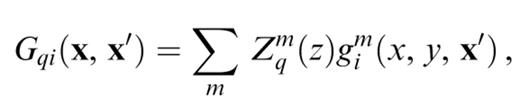
which we express, as done by Friederich et al. (1993), as an operator,
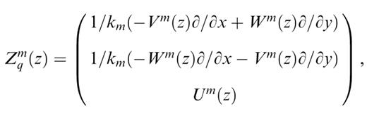
acting on a potential,
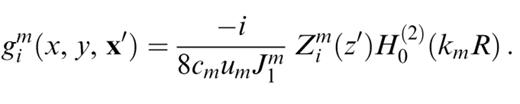
Um, Vm and Wm are the three components of the eigenfunction of mode m. km, cm, um and J1m are its wavenumber, phase velocity, group velocity and energy integral, respectively. x, y and z denote the three components of x in a right-handed coordinate system where x and y are the two horizontal directions and z points downwards. R is the distance in the horizontal plane between x and x′, and H0(2) is the Hankel function of second kind and order 0. In the far-field approximation, the operator Zim(z) simply reduces to a vector containing the eigenfunction of the mode and some π/2 phase factors. In isotropic structures, Um and Vm are respectively the vertical and horizontal components of the Rayleigh wave eigenfunctions, and Wm the eigenfunctions of the Love waves. We note that the operator Z is also present in the expression of the potential, but acting on the source side. In the far-field approximation, the potential can be viewed as simply representing the amplitude and the phase of mode n in the horizontal plane.
Inserting the modal decomposition (14) into eq. (12), we can also write the scattered wavefield of order p as a sum of modes,
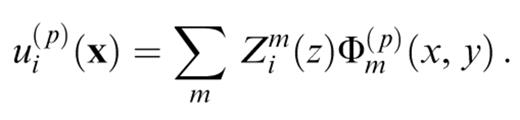
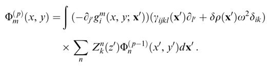
Φm(p)(x, y) is the potential of mode m at scattering order p. Using a similar decomposition for the wavefield scattered at order p−1, and inserting in the scattering equation (12), we obtain a recursive expression for calculating the potentials of the different modes at the different scattering orders,
The advantage of the modal decomposition is that we can separate this volume integral into a combination of a surface and a vertical integral,
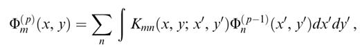
with
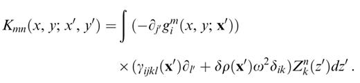
Note that Kmn(x, y;x′, y′) is an operator, in the sense that it contains derivatives to be applied to the potential Φn(p−1)(x′, y′). It is independent of the scattering order, and thereby needs to be calculated only once when we iterate for multiple scattering. In the two next sections, we will analyse the structure of these two integrals and detail the procedure we have followed to compute them.
2.4 Structure of the coupling coefficient
The coupling coefficient Kmn(x, y;x′, y′) expresses how a heterogeneity located at (x′, y′) transfers energy from mode n to mode m, and how this energy is observed at (x, y). In the general anisotropic case, we have 21 independent combinations of indexes for which the coupling has to be calculated. If the reference structure is isotropic, the potential of the Green's function gim(x, y;x′) and the form of the Zkn operators are given by eqs (16) and (15) respectively. Inserting them into eq. (20) and developing some arithmetic, one can obtain the detailed expression of the coupling of Love and Rayleigh modes by an anisotropic heterogeneity. Developing the differentiation in (−∂j′gim(x, y;x′)) leads to first- and second-order derivatives of the Hankel function present in gim(x, y;x′). Applying the operators (Zkn(z′)) and (∂l′Zkn(z′)) to the potential Φn(p−1)(x′, y′) leads to terms in the potential and in its first- and second-order derivatives with respect to the horizontal coordinates. The coupling therefore has the following general structure:
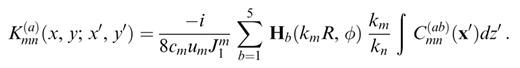
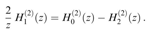
The index a can take six different values and indicates whether the element K(a)mn(x, y;x′, y′) is to be multiplied by the potential of mode n or by one of its first- or second-order horizontal derivatives. Hb(kmR, φ) is one of the five functions H0(2)(kmR), H1(2)(kmR) cos(φ), H1(2)(kmR) sin(φ), H2(2)(kmR) cos(2φ) and H2(2)(kmR) sin(2φ), as indicated in Tables 1–4. φ is the azimuth of (x, y) as seen from (x′, y′), counted positively clockwise from the x-direction. These functions express the azimuthal pattern and the propagation of the wavefield scattered to mode m by each single heterogeneity. The higher-order Hankel functions originate from the differentiation of the Hankel function of order 0, and we have used the following relation to reduce some expressions:
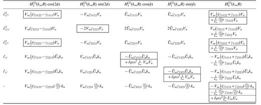
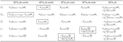
Expressions for Rayleigh to Rayleigh coupling.  and similarly for Um. The terms that are not zero in the isotropic case are shown in boxes.
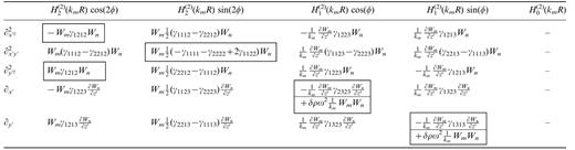
Expressions for Love to Love coupling.
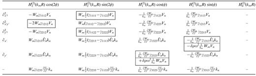
Expressions for Rayleigh to Love coupling.
Expressions for Love to Rayleigh coupling.
The elements Cmn(ab)(z′) are depth integrals of combinations of elastic coefficients, density perturbations and eigenfunctions of modes m and n. Their expressions are given in Tables 1–4. They express how the heterogeneity transfers energy from mode n to m at (x′, y′).
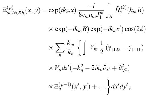
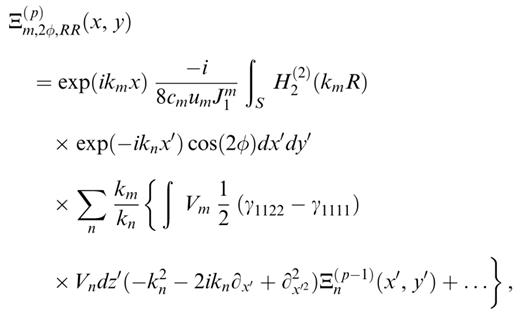
As an example, let us write, in the potential of mode m scattered at order p, the term which varies in cos(2φ), for Rayleigh–Rayleigh coupling. Inserting elements in the first column of Table 1 into eqs (19) and (21), we obtain
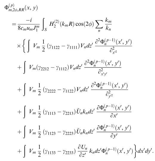
The elements that do not reduce to zero when the heterogeneity is isotropic are shown in boxes in Tables 1–4. Our results reduce to those obtained by Friederich et al. (1993) in the case of isotropic heterogeneities and Rayleigh–Rayleigh coupling. Replacing the Hankel functions by their far-field approximations, we also recover the coupling expressions given by Snieder (1986) for isotropic heterogeneities and single scattering.
Anisotropy introduces a large number of additional terms in comparison with isotropic heterogeneities. We note in particular that the symmetry in the coupling between Love and Rayleigh modes is broken by the anisotropy.
In order to analyse the structure of the coupling, it is useful to define a principal direction of propagation in the structure. In the examples presented in the next sections, the source of the displacement is a plane wave incident on the heterogeneous structure in the x-direction. φ=0 therefore defines the forward direction. The reference wavefield varies only in the x-direction and the terms that contain partial derivatives of the wavefield in the y′-direction are zero at the first scattering order. For isotropic heterogeneities, we obtain the same results as Snieder (1986) concerning the azimuthal variation of the scattering: Rayleigh to Love and Love to Rayleigh coupling have an azimuthal dependence in sin(φ) and sin(2φ) only, producing no coupling in the forward direction. Unlike in the isotropic case, Love to Rayleigh and Rayleigh to Love coupling in the anisotropic model have elements in cos (2φ) in cos (φ), and without dependence in φ. They are therefore able to produce mode coupling in the forward direction. In the case of large heterogeneities, forward scattering becomes dominant, and these elements are able to produce significant polarization anomalies, as we will see in the examples presented in Section 4.
2.5 Differentiation and integration in the horizontal plane
Eq. (23) and similar equations for other mode combinations and azimuthal variations contain horizontal derivatives of the potentials and an integration in the horizontal plane. In this section, we give some details on the procedures we have followed to perform these two operations in a stable and efficient way.
In the examples we have analysed, the incoming wavefield is a plane wave propagating along the x-axis. The potential of each mode of the reference wavefield can therefore be expressed as a constant amplitude and a simple phase variation,
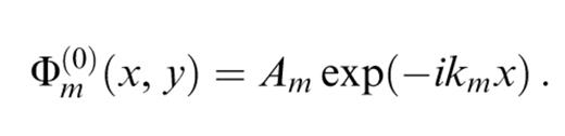
For higher orders of scattering, the horizontal variations of the wavefield are of course much more complicated, but for large-scale heterogeneities, forward scattering is expected to dominate (Friederich et al. 1993). Removing the expected dominant phase from the potential of each mode by writing
enables us to work with the quantity Ξm(p)(x, y), which is expected to vary more smoothly than Φm(p)(x, y). It is therefore possible to evaluate and differentiate it numerically with a smaller number of gridpoints. In order to perform the numerical differentiations, we have used simple low-order schemes.
The total scattered wavefield is a sum of the wavefields scattered by the heterogeneities distributed in the total structure. This sum is expressed by the surface integral in eq. (23). It contains Hankel functions and potentials that oscillate rapidly. As we have just seen, it is possible to reduce the oscillations of the potential by using Ξm(p)(x, y) instead of Φm(p)(x, y). The Hankel functions can similarly be decomposed into a rapidly varying phase and a more smoothly varying amplitude,
Inserting this into, for example, eq. (23), we obtain
where  . Note that ∂2x′2 has been transformed into a slightly longer expression. Except for its two exponential functions, the integrand of the surface integral is expected to be relatively smooth. This kind of integral is well suited to be integrated by the Filon integration scheme (Fraser & Gettrust 1984). We give more details on this integration in Appendix A.
The second difficulty associated with the surface integral is related to the singularity of the Hankel functions at R=0. We show in Appendix B that all the integrals involved in eq. (21) are integrable and can be performed analytically close to the origin in R.
This completes the different numerical elements we need in order to be able to compute the coupling operators in eq. (20), the potentials in eq. (19) and finally the wavefields in eqs (17) and (11). In the numerical examples presented below, the eigenfunctions in the reference structures were calculated with programs provided by Saito (1988).
3 Isotropic heterogeneities
We now present results of the coupling method in models with isotropic heterogeneities. We first validate the method by comparing our results for a simple crustal model that has a cylindrical heterogeneity with an exact solution derived by Stange & Friederich (1992). We then analyse how Rayleigh and Love wavefields at 25 s period are deformed when they propagate through some simple geometrical mantle heterogeneities.
3.1 Validation of the method
In order to check the validity of our approach, we first calculate the wavefield produced when a Rayleigh wave at a period of 2π s, with a wavelength of about 18 km, encounters a cylindrical heterogeneity embedded in a simple crustal structure. We use the same model as Friederich et al. (1993), that is, a 5.7 per cent variation in S-wave velocity over the whole depth of the crust within a vertical cylinder of 36 km diameter. We use also the same discretization of the model, with a grid step of 2.8 km, that is, about six gridpoints per wavelength. For this kind of model, Stange & Friederich (1992) derived an exact solution based on a decomposition of the wavefield into propagating and non-propagating modes. This solution can be used to check the validity of approximate methods.
In order to represent the wavefield, we use all the modes that propagate in the structure, that is, three Rayleigh modes and three Love modes. Unlike the exact solution, energy scattered at high incidence angles and propagating in the mantle is not accounted for in our results.
In Fig. 1, we present the amplitude of the vertical wavefield at four different iterations, each iteration representing the addition of one order of scattering (i.e. N varying from 1 to 4 in eq. 11). At the first iteration, we obtain the wavefield in the Born approximation, which consists of the incoming field and the single-scattered field. We notice that the wavefield varies very little after the second iteration, but that there is a significant variation between the first and the second iterations, especially in the amplitude on the lateral heterogeneity itself. The Rayleigh wave fundamental mode accounts for 95 per cent of the total wavefield on the vertical component, justifying the assumption made by Friederich et al. (1993) that mode coupling was not very important in that case. Comparing with the exact solution given in Fig. 2 of Friederich et al. (1993), we find a very good agreement. The largest difference is situated on the heterogeneous cylinder itself and can be evaluated at 0.03, that is, 7 per cent of the peak-to-peak amplitude variation over the whole figure. The difference is smaller than 1 per cent in most of the figure.
3.2 Scattering of Rayleigh waves
3.2.1. Amplitude in model 1
In Fig. 2, we show the vertical wavefield resulting from a Rayleigh wave fundamental mode with period 25 s, corresponding to nearly 100 km wavelength, propagating through an oceanic model showing a heterogeneity of 10 per cent in S-wave velocity in the upper mantle. The relative P-wave velocity variation is the same as that in the S-wave velocity, and the relative density variation is 4 per cent. The heterogeneity in this model, called model 1, is a vertical body extending from 10 to 100 km depth with a hexagonal section of about 400 km width, as shown in Fig. 2. The geometry has been chosen in order to have vertical boundaries parallel, oblique and perpendicular to the incoming wavefield. The model and the wavefield are sampled every 20 km, ensuring five samples per wavelength.
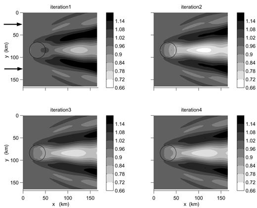
Map in the horizontal plane of the total vertical wavefield at the free surface at iterations 1 to 4 for a Rayleigh wave fundamental mode with period 2π incident on a crustal model with a cylindrical heterogeneity of 5.7 per cent. The black circle indicates the position of the heterogeneity. The Rayleigh wave is incident from the left of the figure, as indicated by the arrows. The amplitude is normalized with respect to the amplitude of the vertical component in the reference laterally homogeneous structure. This figure is to be compared with Fig. 2 of Friederich et al. (1993).
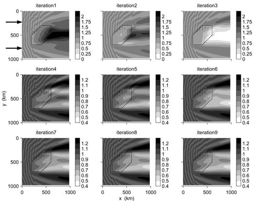
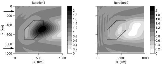
Map in the horizontal plane of the total vertical wavefield at the water bottom after iterations 1 to 9 for a Rayleigh wave fundamental mode with period 25 s incident on model 1 with a heterogeneity of 10 per cent in the lithosphere. The hexagon indicates the position of the heterogeneity. The Rayleigh wave is incident from the left of the figure, as indicated by the arrows. The amplitude is normalized with respect to the amplitude of the vertical component in the laterally homogeneous reference structure. Note that the scaling is different for the first three and the last six iterations.
The wavefield is decomposed on the first four Rayleigh and the first four Love wave modes of the reference structure. The coupling to the higher modes is not very strong and similar results are obtained with, for example, three Rayleigh and three Love modes.
The phase velocity of the Rayleigh wave fundamental mode is 7 per cent higher in the heterogeneous structure than in the reference structure. Propagation through the 400 km wide heterogeneity will therefore modify the phase of the wavefield by about π/2. In the method presented here, any phase difference must be accounted for by the scattering series, and this is equivalent to representing exp(iφ) by its power series. For φ=π/2, the amplitude of the power series of exp(iφ) at the first and second orders reaches values of 1.8 and 1.6, respectively. Including power 3, the amplitude decreases much closer to 1. The series converges within 1 per cent of exp(iφ) in amplitude and in phase using up to power 5, which corresponds to iteration five in the scattering series.
The behaviour of the power series corresponds very well to the behaviour of the scattering series that we observe in Fig. 2, with large amplitudes at the first two iterations, decreasing to smaller values and converging from iteration 3. Iteration 1 corresponds to the Born approximation, which is known to lead to amplitudes that are too large for positive as well as for negative heterogeneities (see e.g. Friederich et al. 1993).
Amplitude variations are very small after iteration 5. Defocusing created by the positive anomaly leads to an amplitude decrease of up to 40 per cent behind the heterogeneity, associated with larger amplitudes in two zones on both sides of the low-amplitude region, corresponding to regions where energy has been deflected.
3.2.2 Amplitude in model 2
The vertical wavefield in a model that we call model 2, similar to the one presented above but with a negative heterogeneity of −10 per cent, is shown in Fig. 3 at iterations 1 and 6. At iteration 1, the amplification of the wavefield is similar to that in model 1, reflecting the fact that it is only an artefact related to the phase variation. The amplitude converges to proper values from iteration 5, and we show here the results at iteration 6.
We observe a strong focusing in a small region behind the heterogeneity surrounded by two shadow zones showing low amplitudes. Although of opposite signs, the orders of magnitude of the amplitude variations in models 1 and 2 are similar. The symmetry in the behaviour of the amplitude at high iteration number, as opposed to the similar patterns at the first iteration, is a good indication that the series converge to the correct wavefields and are not dominated at large iteration number by the pattern related to the phase variation. It appears that the phase variation is a key factor in controlling the number of iterations necessary to reach convergence. The choice of a correct reference model is therefore crucial for the viability of the method.
3.2 Phase variations
The phase delays at iteration 6 are shown for models 1 and 2 in Fig. 4. The order of magnitude corresponds well to that evaluated from the value of the phase velocity in the heterogeneity. For the negative anomaly, the phase delay is slightly larger just behind the anomaly.
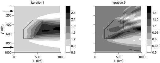
The same as Fig. 2 but for model 2 with a heterogeneity of −10 per cent. The wavefield is shown only at iterations 1 and 6. Note that the scaling is different in the two plots.
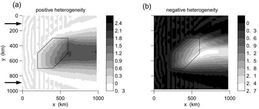
Map of the phase differences between the total vertical wavefields and the reference vertical wavefield at iteration 6. (a) Model 1; (b) model 2. The scale is in radians. The incident wave is a Rayleigh wave fundamental mode.
3.2.4 Mode coupling
The total field presented in the previous figures is a sum of eight modes, but the contribution from the Rayleigh wave fundamental mode is clearly dominant.
For the vertical component, which is less affected by coupling, the fundamental mode accounts for 90 per cent of the total wavefield. The overtones of the Rayleigh wave are generated by coupling inside the heterogeneity and have non-zero amplitude behind the heterogeneity. The amplitude of the first overtone is about 5 per cent of the total wavefield, whereas the second and third overtones account for about 3 and 2 per cent, respectively.
The transverse component is the one most affected by coupling. In Fig. 5, we present the amplitude of the transverse component at iteration 6 in model 1. The total transverse wavefield is represented, as well as the contributions from the Rayleigh wave fundamental mode alone and from the four Love wave modes together. The two dominant features of the transverse wavefield are large amplitudes at the far corners of the heterogeneity, which are mainly related to the Rayleigh wave fundamental mode propagating away from the x-direction, and a zone of large amplitude at the front of the structure, contributed by the Love waves. This last feature is associated with Love waves trapped and partly reflected at the front of the heterogeneity, which is here very strong and very sharp. It also produces large amplitudes associated with boundary effects that contaminate the Love wavefield at x=0. This feature is not stable and grows with iteration number, but disappears from smoother models.
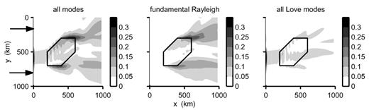
Transverse component at iteration 6 in model 1 for an incident Rayleigh wave fundamental mode. The total wavefield is shown, as well as the contribution from the Rayleigh wave fundamental mode and the four Love wave modes.
3.2.5 Polarization in the horizontal plane
In order to analyse the wavefield in more detail, we present in Fig. 6 the polarization of the wavefield in the horizontal plane in the region where the transverse components have the largest amplitude. The defocusing created by the heterogeneity is clear in Fig. 6. In most places, the polarization in the horizontal plane is rather linear, with deviations from the x-direction simply associated with deviations of the propagation direction of the Rayleigh wave fundamental mode. The polarization has its largest ellipticity inside or close to the heterogeneity. In some places, the transverse component reaches 30 per cent of the horizontal component, but in most of the structure it is below 10 per cent.
3.2.6 Smooth models
The models we have used up to now show sharp boundaries between the reference structure and the heterogeneity, the total variation occurring over a horizontal distance of 20 km. In order to analyse the behaviour of the wavefield in smoother structures, we present the results in models that are 2-D low-pass filtered versions of the previous models in the horizontal plane, with a cut-off wavelength of 300 km.
The resulting wavefields are basically filtered versions of the wavefields propagating in the unfiltered models. As an example, the transverse component at iteration 6 of the wavefield in the model with a positive 10 per cent anomaly is shown in Fig. 7. The amplitude of the trapped Love waves is strongly diminished, but the large amplitude at the far corners of the heterogeneity are still present, similar in magnitude to those in Fig. 5.
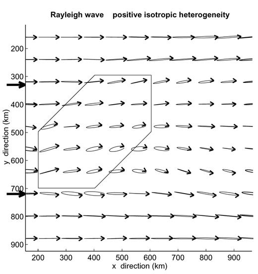
Close-up showing the polarization in the horizontal plane at iteration 6 for an incident Rayleigh wave fundamental mode. The particle motion is shown every four nodes of the model.
The same as Fig. 5 for a model where the heterogeneity is low-pass filtered with a cut-off wavelength of 300 km in the horizontal plane in order to avoid sharp boundaries.
3 Scattering of Love waves
The behaviour of the Love wave fundamental mode is somewhat different from the behaviour of the Rayleigh wave fundamental mode when it propagates through the heterogeneous structures described in the previous sections. The reason is that increasing the S-wave velocity of the reference structure by 10 per cent between Moho depth and 100 km depth, the phase velocity of the Rayleigh wave fundamental mode is modified by 7 per cent, but not its eigenfunction. On the other hand, the phase velocity of the Love wave fundamental mode increases by only 2 per cent, but its eigenfunction is strongly modified. Whereas the energy is evenly distributed between the surface and 200 km depth in the reference structure, the 10 per cent velocity increase in the lid produces a low-velocity zone below, where energy becomes strongly trapped. This results in very different local eigenfunctions in the reference structure and in the heterogeneity, which in turn produces strong reflections and mode coupling at their boundary.
In the models with a sharp boundary between the heterogeneity and the reference structure, we observe strong reflections of the Love wave fundamental mode when it hits the heterogeneity. These reflections dominate the wavefield from iteration 3, and increase in amplitude with iteration number. The way we deal with phases in the algorithm (see eq. 25) is convenient for sampling efficiently wavefields propagating forwards in the x-direction, but not for reflected wavefields. In cases with large reflected wavefields, it would be more appropriate to integrate directly the amplitudes Φm(p) and not the phase-corrected Ξm(p). In the present case, the sampling every 20 km is too sparse for a correct representation of the reflected wavefields.
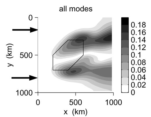
In the models that are low-pass filtered with a cut-off wavelength of 300 km, the reflected wavefields are much smaller and the wavefields converge. We show in Fig. 8 the transverse component of the wavefield at iterations 1 and 9 in the model with a positive heterogeneity. Convergence is not reached before iteration 9 due to oscillations in the amplitude of the fundamental mode of the Love wave. We observe large amplitudes at iteration 1, changing to low amplitudes behind the heterogeneity at iteration 9. Small reflections are still present, giving the characteristic oscillating pattern in front of the heterogeneity. The defocusing behind the heterogeneity is stronger than in the case of the Rayleigh wave fundamental mode. The total wavefield is actually a destructive interference between the fundamental mode, which has an amplitude relative to the reference wavefield of about 0.8, and the three overtones of the Love wave, which have maxima amplitudes of 0.8, 0.3 and 0.1. The overtones dominate in a 300 km wide zone at the rear of the heterogeneity, leading in this region to polarities of the Love wavefield opposite to the polarity one would obtain in the reference model. The coupling to Rayleigh waves is moderate and produces a vertical wavefield of about 10 per cent of the transverse one.
Transverse component of the total wavefield at iterations 1 and 9 for a Love wave fundamental mode incident in a low-passed model with a heterogeneity of 10 per cent.
In the case of a negative low-pass-filtered heterogeneity, mode coupling is also a dominant characteristic of the wavefield. We show in Fig. 9 the transverse component of the total wavefield, the contribution from the Love wave fundamental mode and the sum of the contributions from the three Love wave overtones. We observe a strong focusing behind the heterogeneity in the total wavefield, but we note that most of the energy is on overtones and not on the Love wave fundamental mode, which shows an amplitude low behind the heterogeneity.
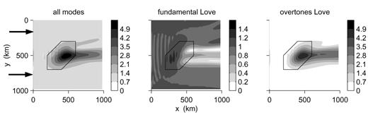
The same as Fig. 8 in a low-passed model with a heterogeneity of −10 per cent. Only iteration 9 is shown. The total wavefield as well as the contributions from the Love wave fundamental mode and from the Love wave overtones are shown.
The polarization in the horizontal plane is shown in Fig. 10. The strong focusing is also clear in this figure. Locally, the polarization can become an important radial component, but the polarization remains basically transverse in most of the structure.
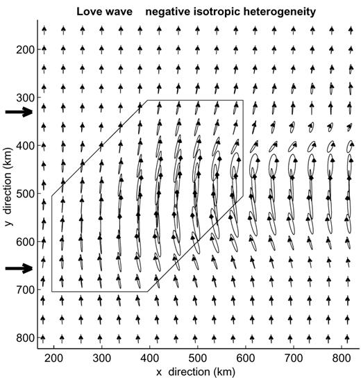
The same as Fig. 6 for an incident Love wave fundamental mode in a low-passed model with a heterogeneity of −10 per cent. Iteration 9 is shown. The particle motion is shown every two nodes of the model.
4 Anisotropic heterogeneities
We now examine the influence of anisotropic heterogeneities on Rayleigh and Love wavefields. For that purpose, we first analyse the effect of the 21 elastic coefficients individually. Although no realistic material has only one elastic coefficient deviating from isotropy, and it is unlikely that we will ever be able to constrain the 21 elastic coefficients in the Earth, we choose to analyse the wavefield perturbations caused by the 21 coefficients individually in order to obtain a comprehensive overview of the possible effects of anisotropy. By being able to single out which coefficients are able to produce wavefields characteristic of anisotropic structures, the effect of any realistic anisotropic structure can then be assessed by a simple examination of the value of a few of its elastic coefficients in the coordinate system defined by the wave propagation direction. At the end of this section, we study the wavefields in simple models containing oriented mantle minerals.
4.1 Individual elastic coefficients
We use in this case a very simple geometrical model where the heterogeneity is a cube extending from 10 to 200 km depth over a 600 by 600 km square in the horizontal plane. In this region, one of the elastic coefficients is modified by 10 GPa, which is of the order of magnitude of the anisotropy in several mineral elastic tensors (see e.g. Babuska & Cara 1991). A similar variation in the Lamé coefficient μ would correspond to an S-wave velocity variation of 5.8 per cent. However, since we modify only one element of the elastic tensor at a time, it actually corresponds to a smaller heterogeneity. The reference structure is the same as in the previous section. The model is sampled every 20 km and we also use four Rayleigh modes and four Love modes to represent the wavefield.
We calculate the wavefields up to iteration 4, but in all cases except for C1312, convergence is reached with two iterations and the wavefield at the first iteration gives a very good approximation to the total wavefield. This means that the features we observe can be predicted easily by examination of Tables 1–4, taking into account that the incoming wavefield does not vary in the y-direction. Perturbation of an elastic coefficient that is involved only in coupling terms containing y-derivatives of the wavefield does not perturb the wavefield. This is the case for example for C2223 for an incident Rayleigh wave, and for C1313 for an incident Love wave. A number of other elastic coefficients couple Rayleigh modes together, Love modes together, or couple Rayleigh and Love modes with a sine function in the azimuthal variation. All these coefficients modify the wavefields in a similar fashion to isotropic heterogeneities, and we will not analyse them in detail here.
The elastic coefficients that produce wavefield perturbations characteristic of anisotropy are those that couple Love and Rayleigh waves in a term with no azimuthal variation or with a variation in cosine. In that case, we have coupling between Love and Rayleigh waves in the forward direction, a feature that does not exist in isotropic structures. When propagating through the anisotropic structure, some signal builds up on the transverse components for incident Rayleigh waves, and some radial and vertical components build up for incident Love waves.
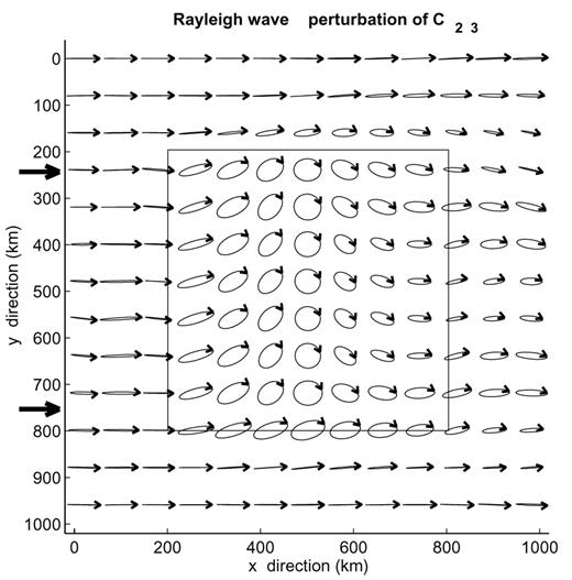
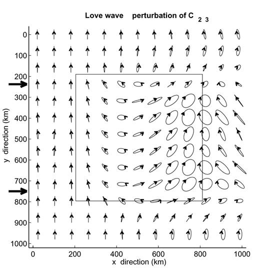
These different coefficients modify the wavefield in different ways depending on the phase relation between the incoming and the scattered waves. For small coupling, the phase relation is such that the polarization in the horizontal plane either remains linear, but at an angle with respect to the radial or transverse direction, or becomes elliptic. For example, C1112, C2313 and C3312 couple Rayleigh to Love waves in such a way that their two horizontal components are mostly in-phase. This produces a linear polarization in the horizontal plane as shown in Fig. 11 for C3312 and an incident Rayleigh wave fundamental mode. The transverse component, which is mostly confined to the heterogeneity, reaches 25 per cent of the radial component and produces a clockwise deviation of the polarization in the horizontal plane. The same C3312 coefficient produces a stronger and more complex polarization anomaly on Love waves, as shown in Fig. 12. In that case, the initially transverse polarization first becomes strongly elliptic inside the anisotropic region and then returns to linearity at the rear of the structure, but with a significant radial component. The amplitude ratio between the radial and transverse components reaches 60 per cent in that case, of which 75 per cent is on the Rayleigh wave fundamental mode.

The same as Fig. 6 for an incident Rayleigh wave fundamental mode in a model with a perturbation of C3312 by 10 GPa in the area indicated by the black square. Iteration 4 is shown.
The same as Fig. 11 for an incident Love wave fundamental mode.
Except for C1312, which we will discuss separately, the other coefficients produce smaller polarization anomalies than C3312. 10 GPa perturbations on C1112 and C3213 produce polarization anomalies very similar in shape to those produced by C3312, but with smaller amplitudes: the maximum amplitude ratios reach 12 and 23 per cent respectively for an incoming Rayleigh wave fundamental mode, and 40 and 15 per cent respectively for an incoming Love wave fundamental mode.
C1123 and C3323 couple the waves in such a way that an incoming Rayleigh wave gets an elliptic polarization in the horizontal plane, but the transverse to radial amplitude ratio remains small, reaching only 5 and 6 per cent respectively. They produce radial components of only 4 per cent for an incoming Love wave. C2223 and C2221 also produce coupling from Love to Rayleigh waves in the forward direction, but in two terms in cos(2φ) and 1 that cancel each other at first order. The resulting wavefield perturbation is not significant.
The main contribution to the polarization anomaly of a Love wave fundamental mode is usually on the Rayleigh wave fundamental mode or on the first Rayleigh wave overtone. In all the cases that we have examined, the truncation to four Rayleigh modes gives satisfactory results. Similarly, we have verified that four Love waves are sufficient to represent the polarization anomalies for an incident Rayleigh wave fundamental mode. The largest amplitude is usually on the fundamental mode or first overtone of the Love wave in that case.
4.1.1 C1312
The elastic coefficient C1312 appears to be the most effective one to couple Love and Rayleigh waves together. The horizontal polarization of the wavefield for an incident Rayleigh wave in a model with a 10 GPa perturbation in C1312 is shown in Fig. 13, and the wavefield for an incident Love wave is shown in Fig. 14. In both cases, we observe a complex wavefield with a generalized polarization varying from radial to transverse and elliptic. Convergence is reached more slowly with this elastic coefficient than with the other ones. The wavefields presented in Figs 12 and 13 include nine orders of scattering, but six orders give very similar results.
The same as Fig. 11 for a perturbation of C1213. Iteration 9 is shown.
The same as Fig. 13 for an incident Love wave fundamental mode.
A 5 GPa perturbation of C1312 gives somewhat simpler wavefields, but the transverse component still reaches 50 per cent of the radial component for an incident Rayleigh wave. For an incident Love wave, the radial component still dominates the radial component locally. In both cases, the polarizations are strongly elliptic.
4.2 Oriented pyrolite models
No material is such that deviation from isotropy is on only one elastic coefficient, and we will now examine the polarizations in physically realistic models of anisotropy. However, the analysis of the influence of the different elastic coefficients gives us some clues on which physical models produce characteristic wavefield variations, i.e. strong polarization anomalies. Materials showing a significant C1312 are clearly the best candidates, followed by materials with non-zero C3312 and C3213 elastic coefficients.
Instead of perturbing one elastic coefficient, we now fill the 600×600×190 km cube of the preceding section with partially oriented minerals. We use the elastic coefficients given by Estey & Douglas (1986) for a mantle of pyrolitic composition, with 59 per cent olivine, 12 per cent garnet and 29 per cent pyroxene. The isotropic mean of the structure is kept equal to the value in the reference structure. The anisotropy in the model is constant with depth, equal to 50 per cent of the deviation of the pyrolite elastic tensor with respect to its isotropic mean. This simulates a pyrolitic mantle with 50 per cent oriented crystals, producing a 7 per cent P-wave velocity anisotropy. Anisotropy may reach these values locally in the mantle, and although quite extreme, this model is not unrealistic. The anisotropy of the olivine crystals actually dominates the anisotropy of the pyrolite, and very similar results are obtained with models containing 30 per cent oriented olivine crystals.
Pyrolite has a quasi-hexagonal orthorhombic structure with the olivine a-axis aligned with the axis of quasi-hexagonal symmetry. These two axes become dominantly oriented in the flow direction of the mantle (see Mainprice et al.2000, for a recent review of the subject).
4.2.1 Horizontal symmetry axis
When the hexagonal symmetry axis remains horizontal, the C1312 coefficient remains equal to zero, and the polarization anomalies associated with the anisotropy remain small. The amplitudes of the two horizontal components of the wavefield for an incoming Rayleigh wave fundamental mode in a model with the symmetry axis oriented at 45° to the x-direction are shown in Fig. 15. We notice that the transverse component remains small compared to the radial component, reaching at the most 10 per cent. The transverse component is largest in the anisotropic region. It is mostly in phase with the radial component, giving a linear polarization with a slight clockwise rotation with respect to the x-direction. In addition to producing a polarization anomaly, the anisotropy deviates the direction of energy propagation clockwise, as can be seen by the location of the amplitude maximum and minimum of the radial component.
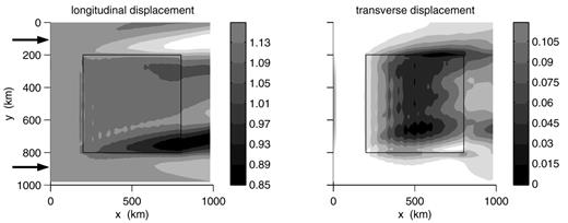
Radial and transverse components of the total wavefield for a Rayleigh wave fundamental mode incident on a model with a heterogeneity due to 50 per cent oriented pyrolite with quasi-hexagonal symmetry axis oriented in the horizontal plane at 45° to the x-axis. The oriented pyrolite is located in the region delimited by the black square.
In this model, an incident Love wave fundamental mode gets a radial component mostly in phase with its transverse component and that reaches about 25 per cent in amplitude. It also gets a vertical component of the same order of magnitude. As expected, results with a mirror symmetry with respect to the x-direction are obtained when the symmetry axis is oriented at −45° to the x-direction.
Using the method of Thomson (1997) and associated code, we calculated the surface wave eigenfunctions in a laterally homogeneous structure with the same characteristics as the anisotropic part of our model. This is a way to verify our code and to analyse the relation between polarization anomalies in laterally homogeneous and heterogeneous structures. The first eigenfunction in that model, corresponding to a quasi-Rayleigh wave fundamental mode, has a quasi-linear polarization in the horizontal plane rotated clockwise with respect to the radial direction, with a transverse component equal to 21 per cent of the radial component. The second mode, a quasi-Love wave fundamental mode, has a radial component equal to 10 per cent of the transverse component. The polarization anomalies have the same sign as in our results. Although the amplitudes are somewhat different, the order of magnitude of the polarization anomalies is similar.
4.2.2 Tilted symmetry axis
Tilting the symmetry axis relative to the horizontal plane leads to a non-zero value for C1312, resulting in much larger polarization variations. The polarization in the horizontal plane for an incident Rayleigh wave in a model with 50 per cent oriented pyrolite with a symmetry axis tilting at 45° to the horizontal, in a vertical plane oriented at 45° to the x-direction, is shown in Fig. 16. We observe a prograde elliptic polarization, with the ellipse's large axis gradually varying in direction across the structure. The amplitude of the transverse component reaches 47 per cent of that of the radial component.
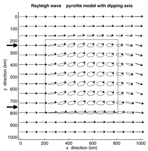
The same as Fig. 11 for a heterogeneity due to 50 per cent oriented pyrolite with quasi-hexagonal symmetry axis dipping at 45° to the horizontal plane, in a vertical plane oriented at 45° to the x-axis.
Using the code of Thomson in a laterally homogeneous structure of oriented pyrolite with a tilted axis, we find that the quasi-Rayleigh wave fundamental mode in that structure also has a prograde elliptic motion. The transverse component is equal to 90 per cent of the radial component, which means that the ellipse nearly reduces to a circle. This is similar to what we observe, when the wave reaches the far end of the anisotropic region. Using a heterogeneous structure, more complex features can of course be modelled, such as the width of the transition zone where the polarization anomaly builds up, and the interference pattern that occurs behind the anisotropy. However, the two codes give compatible results.
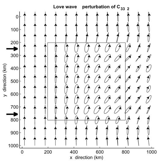
The polarization anomalies observed for an incident Love wave fundamental mode in a model with a tilted axis are very large (Fig. 17). The polarization gradually rotates from transverse to dominantly radial via a retrograde elliptic motion. A vertical component also gradually builds up inside the anisotropic region and reaches an amplitude of 150 per cent relative to the transverse amplitude in the reference structure. In a laterally homogeneous structure, the quasi-Love wave fundamental mode also shows a retrograde elliptic motion but the transverse motion remains dominant: the radial and vertical components of the surface polarization are respectively 33 and 15 per cent of the transverse component.
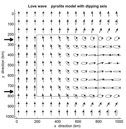
The same as Fig. 16 for an incident Love wave fundamental mode.
Tilting the pyrolite symmetry axis away from the horizontal plane modifies the polarization dramatically. A similar observation was made by Kirkwood & Crampin (1981) in laterally homogeneous structures and by Park (1997) on long-period surface waves. On the other hand, it does not modify significantly the azimuthal dependance of the phase velocity and the direction of greatest phase velocity. Classical surface wave tomography, based on inversion of the phase velocity, is therefore not well-suited for determining the inclination of the axis in the vertical plane, and can benefit from the complementary information that polarization anomalies can bring.
5 Conclusions
We have presented a multiple-scattering method to model the propagation of surface waves in 3-D isotropic and anisotropic heterogeneous structures. Since no far-field approximation is made, the heterogeneity may be located anywhere in the structure, including around the source or in the vicinity of the receiver. The wavefield is decomposed on the eigenfunctions of a reference structure and expressed as a scattering series. The heterogeneity modifies the phases and amplitudes of the modes and couples them together.
We have first verified the method by comparing its results with those of an exact method for a vertical cylindrical heterogeneity embedded in the crust. The performance of the method has then been analysed for various mantle models with strong isotropic and anisotropic heterogeneities. We have studied the wavefield resulting from plane Rayleigh and Love wave fundamental modes at 25 s period incident on structures with 10 per cent perturbation in S-wave velocity and anisotropic heterogeneities extending over several wavelengths. We have shown that the scattering series usually converges despite the strength of the heterogeneity used in these models. Several orders of multiple scattering are nonetheless necessary to obtain a good representation of the wavefield in the most severe cases, where the single-scattering approximation would not be appropriate.
In order to save computing time, we have used Filon integration extensively when implementing the method. This is well suited to handle cases with an incident plane wavefield and a dominant forward scattering, but is not well suited to handle large reflected waves. The implementation can easily be modified by returning to classical integration in order to be better suited for such cases. Classical integration would also be better suited to analyse the wavefield resulting from a source embedded in a heterogeneous region, in order to analyse the observations of Van der Lee (1998), for example.
The computations can easily be performed on an ordinary workstation. For one period, the computing time depends mainly on three factors: the number of scattering iterations, the number of modes squared and the number of gridpoints squared. The depth dependence of the model has no significant influence on the computing time. As an example, each iteration in the anisotropic cases presented in Section 4, with eight modes and 2500 gridpoints, ran in 40 min on a DEC-PWS500au workstation. The computer programs associated with this work will be made available on request to the author ([email protected]).
We have also obtained important results concerning the difference between wavefield perturbations caused by isotropic and anisotropic heterogeneities. In models with isotropic heterogeneities, the phase and amplitude of the wavefield vary strongly, but polarization anomalies remain small. On the other hand, models with realistic anisotropic heterogeneities may produce very strong polarization anomalies, leading to transverse components on the Rayleigh wave that have the same order of magnitude as the radial component or large vertical components for the Love waves. Our formalism allows a detailed analysis of the different types of wavefield perturbations that the individual elastic coefficients produce, and single out which elastic coefficient must be non-zero for polarization anomalies to appear. We show in particular that olivine produces very different polarization anomalies if its fast axis is oriented horizontally or at an angle with respect to the horizontal plane, and that polarization analysis provides information that complements the information obtained using phase velocity.
Except for the Rayleigh wave fundamental mode in purely isotropic structures, mode coupling is an important feature of surface wave propagation in the heterogeneous structures presented here, and could not have been neglected.
Acknowledgments
I wish to thank Colin Thomson for providing a copy of his code for calculating modes in laterally homogeneous anisotropic structures. Thanks also to Wolfgang Friederich and Jeffrey Park for their reviews.
Appendices
Appendix A: Integration in the horizontal plane by the Filon method
Filon integration (Fraser & Gettrust 1984) is a method that performs efficiently integrals of the form
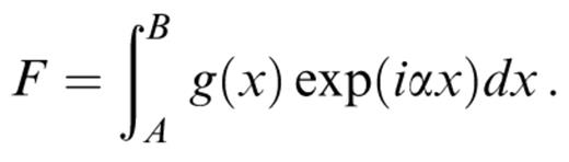
Eq. (27), which we have to solve, has a more complicated form,
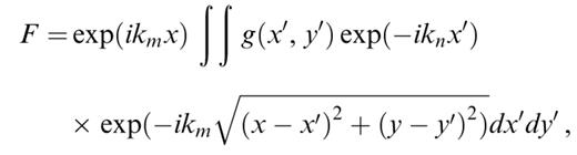
where g(x′, y′) is a smooth function in x′ and y′. Performing the change of variable =x′−x and  , the integral becomes
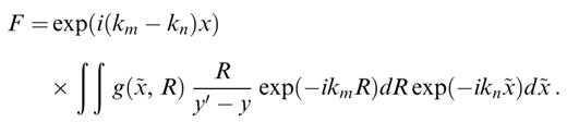
For values of y′−y that are not close to zero, the function g(, R)[R/(y′−y)] varies smoothly in the horizontal plane, and the integral is in a form suitable for using the Filon integration method twice.
For values of y′−y that are close to zero, the function g(, R)[R/(y′−y)] has a singularity and this change of variable is not suitable. In that case, exp(−ikmR) does not vary strongly with y′. Reorganizing eq. (A2) in order to extract the dominant phase variation in from the integral in y′, we obtain
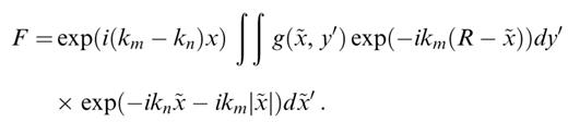
Since g(, y′) exp(−ikm(R−)) is smoothly varying both in y′ and in , we can use an ordinary integral in y′ and an ordinary or a Filon integral in depending on how strongly varying the function exp(−ikn−ikm||) is.
Appendix B: Analytical integration of the Hankel functions close to the origin
Close to R=0, the Hankel functions are singular and the integral (21) requires special attention. In practice, we use the numerical scheme described in Appendix A to perform the integral on the whole surface except on a small square defined by the eight gridpoints neighbouring the observation point (x, y). On that small square, the integrals are performed mainly analytically and partly numerically, as described in this Appendix.
We assume that the variations of the potential Ξ and of the structure in that small square are small enough that they can be neglected. One can therefore move a number of terms outside the surface integral of eq. (27), for example, which becomes
where we have reinserted the classical Hankel function (eq. 26). As we will now show, the surface integral in this equation can be evaluated analytically on any disc centred on R=0. We therefore perform the integral analytically on a disc centred on R=0 and with radius A equal to the grid step. We complete the integral on the small square by a numerical integration of the function in the four remaining corners, where the functions are not singular.
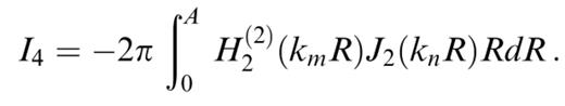
In order to perform the analytical integration on the disc, and considering all the terms present in eq. (21), we need to evaluate the following five integrals:
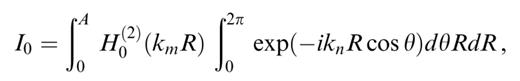
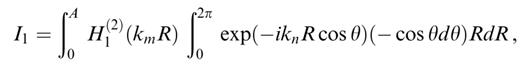
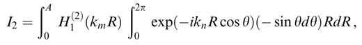
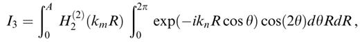
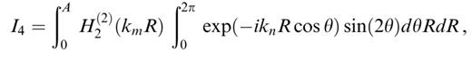
where we use θ=φ+π instead of φ in order to remain as close as possible to classical conventions in cylindrical coordinate systems.
The integrals in θ are easily performed using the decomposition of exp(−iknR cos θ) in terms of Bessel and trigonometric functions given in eqs (9.1.44) and (9.1.45) in Abramowitz & Stegun (1972). The results are
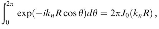
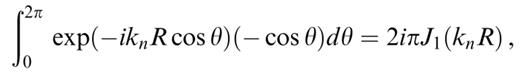
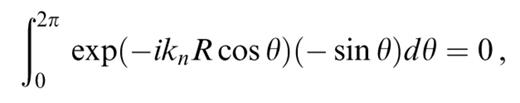
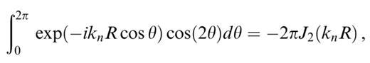
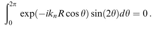
We are left with having to evaluate the three following integrals:
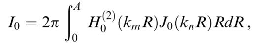
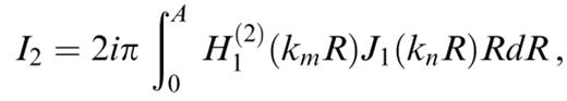
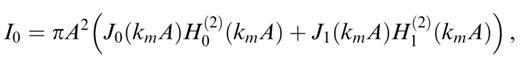
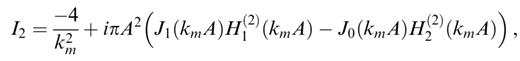
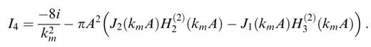
Transforming the Hankel functions into modified Bessel functions according to formula (9.6.4) in Abramowitz & Stegun (1972) and using the formula (6.521.4) for integrals of products of Bessel and modified Bessel functions in Gradshteyn & Ryzhik (1980), we obtain the following results:
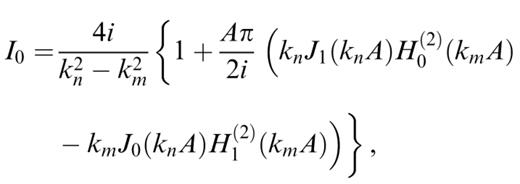
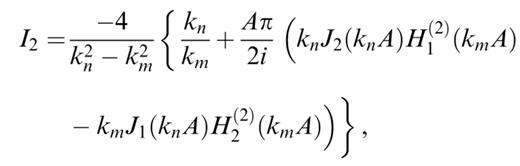
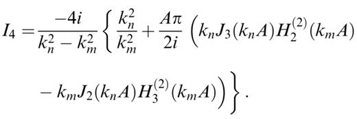
These expressions can be used only for calculating the coupling of two different modes, with different kn and km. In order to evaluate these expressions in the case kn=km, we calculate the value of the expressions when kn→km and obtain
We have verified numerically the correctness of these expressions. It can also be shown that these integrals tend to zero when A tends to zero, meaning that the field scattered by an infinitely small disc tends to zero.
References
