


Summary
Wavefront healing is a ubiquitous diffraction phenomenon that affects cross-correlation traveltime measurements, whenever the scale of the 3-D variations in wave speed is comparable to the characteristic wavelength of the waves. We conduct a theoretical and numerical analysis of this finite-frequency phenomenon, using a 3-D pseudospectral code to compute and measure synthetic pressure-response waveforms and ‘ground truth’ cross-correlation traveltimes at various distances behind a smooth, spherical anomaly in an otherwise homogeneous acoustic medium. Wavefront healing is ignored in traveltime tomographic inversions based upon linearized geometrical ray theory, in as much as it is strictly an infinite-frequency approximation. In contrast, a 3-D banana–doughnut Fréchet kernel does account for wavefront healing because it is cored by a tubular region of negligible traveltime sensitivity along the source–receiver geometrical ray. The cross-path width of the 3-D kernel varies as the square root of the wavelength λ times the source–receiver distance L, so that as a wave propagates, an anomaly at a fixed location finds itself increasingly able to ‘hide’ within the growing doughnut ‘hole’. The results of our numerical investigations indicate that banana–doughnut traveltime predictions are generally in excellent agreement with measured ground truth traveltimes over a wide range of propagation distances and anomaly dimensions and magnitudes. Linearized ray theory is, on the other hand, only valid for large 3-D anomalies that are smooth on the kernel width scale √(λ L). In detail, there is an asymmetry in the wavefront healing behaviour behind a fast and slow anomaly that cannot be adequately modelled by any theory that posits a linear relationship between the measured traveltime shift and the wave-speed perturbation.
1 Introduction
During the past decade we have witnessed remarkable progress in the determination of the Earth's 3-D compressional- and shear-wave velocity structure by means of global seismic traveltime tomography. Linearized geometrical ray theory has provided the basis for the majority of these traveltime tomographic studies (e.g. Inoue et al. 1990; Su & Dziewonski 1992; Pulliam et al. 1993; Grand 1994; Masters et al. 1996; Van der Hilst et al. 1997; Su & Dziewonski 1997; Grand et al. 1997; Vasco & Johnson 1998; Boschi & Dziewonski 2000). In this approximation, the traveltime shift of a body wave depends upon the 3-D perturbation in wave speed along the unperturbed, spherical-earth ray path only. A few recent analyses have sought to overcome the limitations of linearization by making use of an iterative inversion procedure, which requires the computationally intensive tracing of rays through the previous 3-D structure (e.g. Bijwaard & Spakman 2000; Widiyantoro et al. 2000). Both linearized and ‘exact’ geometrical ray theory are, however, strictly valid only in the limit of an infinite-frequency wave. The measured traveltimes of actual finite-frequency seismic waves differ from the predictions of ray theory in two significant respects.
First, as a result of diffractive effects, the traveltimes of finite-frequency waves are sensitive to 3-D wave-speed perturbations off the geometrical ray (Woodward 1992; Marquering et al. 1999; Dahlen et al. 2000; Hung et al. 2000; Zhao et al. 2000). A remarkable feature of the 3-D Fréchet kernel expressing this sensitivity is that it is identically zero everywhere along an unperturbed P or S ray; the strongest sensitivity is in fact within a tubular ‘skin’ surrounding the turning ray. The 3-D geometry of a P- or S-wave traveltime kernel resembles that of a hollow banana; in a cross-sec perpendicular to the unperturbed ray, the shape resembles that of a doughnut. Because of these similarities, we have whimsically christened our formalism for computing 3-D traveltime sensitivity kernels, banana–doughnut theory. The original papers describing the theory (Dahlen 2000; Hung et al 2000) will henceforth be referred to as Banana–;Doughnut I and II.
Second, an infinite-frequency wave that accrues a traveltime advance or delay upon passage through a fast or slow anomaly somewhere along its ray path ‘remembers’ that shift as it continues to propagate towards the receiver. This familiar but fundamental aspect of geometrical ray theory can be regarded as the central tenet of seismic tomography (see Fig. 1). In a linearized inversion, a single traveltime-shift measurement only constrains the line integral of the slowness perturbation along the unperturbed, spherical-earth ray; data from millions of crossing ray paths must be fitted simultaneously in order to determine the locations and magnitudes of 3-D wave-speed anomalies within the Earth's mantle. The traveltimes of actual finite-frequency waves violate the central tenet of seismic tomography, due to another intrinsic diffraction phenomenon—wavefront healing—which occurs whenever the scale of any geometrical irregularities in a wavefront are comparable to the wavelength of the wave. If an initially irregular, finite-frequency wavefront continues to propagate through a medium that is devoid of wavelength-scale 3-D heterogeneity, diffraction acts to ‘fill in’ or ‘heal’ the irregularities (e.g. Gudmundsson 1996).
Nolet & Dahlen (2000) conducted a simplified analysis of wavefront healing, using an elementary Gaussian-beam solution to the one-way, parabolic wave equation to investigate the evolution of both phase and group traveltimes, following the passage of a monochromatic scalar wave through an isolated anomaly. We present an independent analysis in this paper, showing how the presence of the doughnut hole enables a 3-D traveltime sensitivity kernel to account for the diffractive healing of a broad-band body-wave pulse. Our objective is to delineate the regime within which banana–doughnut theory provides a valid description of observed finite-frequency traveltime shifts, by comparison with ‘ground truth’ traveltimes measured by cross-correlation of a suite of perturbed and unperturbed synthetic seismograms. In the interests of completeness and pedagogy, we also conduct a 3-D ray-theoretical analysis of a number of the examples which we consider. secs 2–4 are devoted to a review of relevant background material, including a description of our numerical method for computing ground truth synthetic seismograms, and a brief summary of both geometrical ray theory and banana–doughnut theory in the context of the problem under consideration. In secs 5–7 we compare a number of different measures of the traveltime shift, for a variety of source–receiver anomaly configurations.
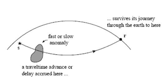
Cartoon illustration of the central tenet underlying conventional traveltime tomography. Diffractive healing of an infinite-frequency wave is negligible, so that a single body-wave traveltime between a seismic source s (star) and receiver r (dot) cannot determine the location of an isolated fast or slow anomaly (grey blob) along the source–receiver geometrical ray.
2 Ground Truth Traveltimes
In the interest of computational expediency, we restrict attention to acoustic-wave propagation in a Cartesian medium. The fundamental principles governing diffraction and wavefront healing are the same regardless of the physical characteristics of the waves. For this reason, we expect the results to be directly applicable to turning P, SV and SH elastic waves in a spherically symmetric background earth model.
2.1 Homogeneous background medium
The background acoustic medium is assumed to be uniform, with a constant-mass density ρ and acoustic wave speed c. The response to an explosive point source in such a homogeneous medium is governed by the classical wave equation,
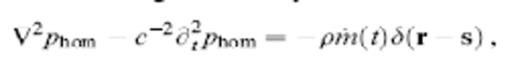
where δ(r−s) is the Dirac delta distribution. The unknown phom(r, t) is the incremental pressure at point r and time t. The quantity m(t) in the source term on the right is the instantaneous rate of change of an infinitesimally small volume dV(t) situated at the point s; the dot denotes differentiation with respect to time. The exact unique solution to eq. (1) in an infinite medium is (Morse & Ingard 1968, sec 7.1)
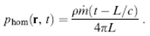
The quantity L = ∥r−s∥ is the straight-line distance between the source, s, and receiver, r. The acoustic pressure response (2) is a delayed pulse that propagates with speed c and is geometrically attenuated by a factor L−1. The shape of the pressure pulse is the second derivative of the differential source volume, m˙(t)=dV¨(t).
2.2 Isolated heterogeneity
To investigate the factors that govern 3-D wavefront healing we consider an extremely simple situation—the passage of a finite-frequency wave through a single, smooth, spherical, cosine-bell ‘inclusion’ in an otherwise homogeneous medium. The anomaly is presumed to have the same constant density, ρ, but a spatially variable wave speed,
Specifically, the fractional wave-speed perturbation is given by

where r is the radial distance from the centre. The dimensionless parameter, ε, is a measure of the strength or magnitude of the wave-speed anomaly; a fast anomaly has ε>0 whereas a slow anomaly has ε<0. The maximum value of the perturbation δc/c at the centre of the sphere, r=0, is
whereas the volumetric root-mean-square average perturbation is
Note that the dimensional parameter a is the diameter rather than the radius of the anomaly. The background wave speed and the uniform density are the same in all of our simulations: c=8 km and ρ=3300 kg m−1, respectively.
2.3 Pseudospectral method
The equations of motion governing acoustic-wave propagation in a constant-density medium are
There are four scalar unknowns in this case, the three Cartesian components of the fluid velocity uhet(r, t) as well as the pressure variation phet(r, t).
We use a parallelized pseudospectral method developed by Hung & Forsyth (1998) to integrate the four equations (7)–(8) numerically. In this technique, the four unknown wavefield variables are represented as discrete 3-D Fourier expansions, enabling the pressure gradient, ∇phet, and velocity divergence, ∇?uhet, in eqs (7)–(8) to be computed by multiplication in the wavenumber domain. Numerical dispersion is significantly improved in comparison to finite difference schemes, which use only a few neighbouring nodes to approximate these spatial derivatives. Wraparound artefacts and unwanted reflections from the eight faces of the 3-D computational grid are suppressed by means of a simple absorbing boundary condition described by Cerjan et al. (1985).
2.4 Model geometry
The spherical anomaly (4) is situated near one corner of a 7650×7650×7650 km3 cube, as depicted in Fig. 2; the number of gridpoints is 256×256×256≈17×106. An explosive point source, m(t), is detonated at a grid point, s, located on the near-corner side of the anomaly and the resulting synthetic pressure response phet(r, t) is sampled at a fan-shaped array of receivers r, stretched across a long diagonal of the cube, so that some of the unperturbed straight rays pass through the anomaly, whereas others do not. We specify the position of an individual receiver, r, by its distance 0≤L≤8000 km from the source, s, and by its azimuth −45°≤φ≤45°, as illustrated in Fig. 3. The distance between s and the centre of the anomaly is denoted by S, whereas that from the anomaly centre to an axial (φ=0°) receiver is denoted by R; the total source–receiver distance is of course just the sum of these two,
The pressure response phet(r, t) at receiver locations, r, between grid points is computed by means of a 3-D bilinear interpolation from the eight adjacent nodal values.
2.5 Source time function
The time variation of the differential source volume in eq. (8) is assumed to be a Gaussian, of the form
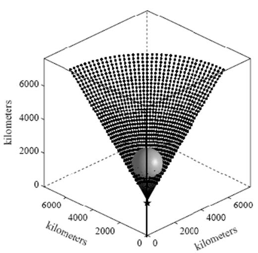
Model configuration and source–receiver geometry used in the pseudospectral simulation of 3-D acoustic-wave propagation. The shaded isosurface represents a smooth, spherically symmetric wave-speed anomaly of the form (4) embedded in an otherwise homogeneous 7650×7650×7650 km3 cube. Solid lines are the unperturbed straight geometrical rays between the point source s (star) and the receivers r (dots). Receivers are spaced every 2.5° along a series of equidistant arcs; the middle (φ=0°) line of receivers lies along the straight ray path through the centre of the spherically symmetric anomaly.
The resulting pressure response (2) in the background homogeneous medium is an acausal two-sided pulse,
with a visually obvious upswing at t≈0 and a characteristic period equal to τ. We denote the associated characteristic angular frequency and wavelength by
respectively. The power spectrum of the source time function (11) is
Note that all three relations (10)–(13) differ slightly from the corresponding eqs (38)–(40) in Banana–;Doughnut II. The upshot of this redefinition is to shift the maximum of |m˙(ω)|2 from  to Ω, so that the characteristic quantities τ, Ω and λ coincide with the visually estimated period, angular frequency and wavelength of the pulse.
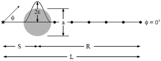
Receiver locations (dots) are completely described by specifying their distance 0≤L≤8000 km from the source (star) and their azimuth −45°≤φ≤45°, measured with respect to the axis of cylindrical symmetry passing through the centre of the spherical anomaly (shaded circle). The quantities S and R are the distances from the anomaly centre to the source s and an axial φ=0° receiver r, respectively. The wave-speed perturbation is a cosine bell of the form (4), having a maximum value (δc/c)max=2ε at the centre r=0, and tending smoothly to zero at r=a/2.
In all of the simulations presented in this paper, the characteristic period and wavelength are
The numerical values (14) and the longest propagation distances, L=8000 km, were chosen to be representative of long-period shear waves that sample the deep mantle. Since the grid spacing is
there are between six and seven grid points per wavelength in the pseudospectral computations; this is more than adequate to ensure numerical accuracy (Hung & Forsyth 1998).
A conventional fourth-order Runge–Kutta scheme is used to advance phet(r, t) and uhet(r, t) in time. The time step Δt must satisfy the von Neumann criterion,
in order for the pseudospectral integration procedure to be stable (e.g. Kosloff & Baysal 1982; Kosloff et al. 1984). We err on the side of conservatism, using a significantly shorter time step,
to ensure that grid dispersion is thoroughly negligible. This and other features of the numerical method, including the efficacy of the absorbing boundary conditions, were checked by comparison with the exact analytical solution (2) for phom(r, t) in an infinite homogeneous (ε=0) medium.
2.6 Dimensionless parameters
Acoustic wave propagation within the simple class of models examined here is completely characterized by four dimensionless parameters:
(i)the magnitude of the anomaly, ε;
(ii)the ratio of the anomaly size to the wavelength, a/λ;
(iii)the dimensionless source–anomaly distance, S/λ; and
(iv)the dimensionless receiver–anomaly distance, R/λ.
To investigate wavefront healing, we generally place the centre of the anomaly at a fixed position relatively close to the source,
and examine the ensuing evolution of the wavefront after it has passed through the anomaly at various receiver distances 0≤R≤30λ and azimuths −45°≤φ≤45°, for a suite of both fast and slow anomaly magnitudes |ε|=3– 12 per cent and dimensions a=λ – 8λ. Only in secs 5.3 and 6 do we alter the location (18) of the anomaly, in order to conduct a brief examination of the principle of source–receiver reciprocity.
2.7 Cross-correlation traveltime measurement
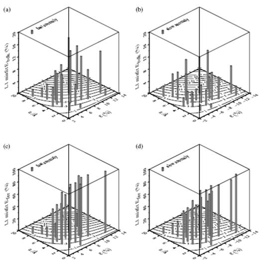
The time required for a wave to propagate from the source, s, to a receiver, r, is measured by cross-correlation of the synthetic waveform, phet(r, t), with the corresponding waveform, phom(r, t), in an infinite homogeneous medium. The traveltime anomaly, δTccm, is the amount by which phom(r, t) must be shifted in time in order to most closely resemble phet(r, t), in the sense
Physically, δTccm is the traveltime of a finite-frequency wave in the perturbed medium relative to its traveltime Thom=L/c in the unperturbed medium. A negative traveltime anomaly, δTccm<0, corresponds to an advance in the arrival of the perturbed pulse phet(r, t) relative to the unperturbed pulse phom(r, t), whereas a positive anomaly, δTccm>0, corresponds to a delay. Unless indicated otherwise, we make use of a boxcar cross-correlation window of length t2−t1=45 s, carefully positioned to ensure that it includes all non-negligible portions of the two τ=25 s pulses phet(r, t) and phom(r, t−δTccm). The value of the traveltime anomaly δTccm is determined by least-squares fitting of a parabola to a discretized version of the cross-correlagram (19) in the vicinity of its maximum.
The quantity δTccm is the first of several measures of the traveltime anomaly due to a wave-speed perturbation of the form (4) which we shall introduce and compare. A different three-letter subscript will be used to identify and distinguish these various measures of δT. The values δTccm measured by cross-correlation (19) are regarded as ground truth standards for the purpose of comparison.
3 Geometrical Ray Theory
In the limit of an infinitely high-frequency pulse, τ→0, the wave can be regarded as propagating from s to r along one or more geometrical rays. The problem of determining the response phet(r, t) reduces to that of tracing all of the rays and computing the geometrical amplitude variation along them.
3.1 Ray tracing
We denote the position and instantaneous propagation direction of a wave along a ray by x and k^, respectively. In the language of classical differential geometry, the unit vector k^ is the tangent vector along the ray. The equations needed to trace rays can be written in a variety of forms, including
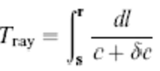
where dl and dT are the differential arclength and traveltime, respectively and ∇⊥=∇−k^k^?∇ is the gradient in a direction perpendicular to the ray (Dahlen & Tromp 1998, sec 15.3). Every ray starts from the source s in a specified direction:
To perform two-point ray tracing, it is necessary to find the set of initial take-off vectors k^s that enable the associated ray to ‘hit’ the receiver r. Fermat's principle stipulates that the geometrical rays between s and r are those paths for which the total traveltime
is stationary. The first-arriving wave propagates along the global least-time path, whereas later arrivals propagate along minimax paths that are stationary but not least-time.
3.2 Ray-theoretical response
The approximate ray-theoretical pressure response is a straightforward generalization of the result (2),
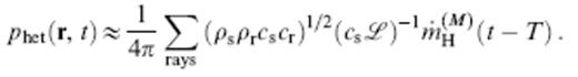
The subscripts on ρs, cs and ρr, cr denote evaluation at the source s and the receiver r, respectively. The summation accounts for the possibility of multipathing, that is, the existence of more than one geometrical ray between s and r. The quantity ℒ(r, s) is a geometrical attenuation or spreading factor, analogous to the straight-line source–receiver distance L=∥r−s∥ in a homogeneous medium. If dΣ is the differential cross-secal area at the receiver r of an infinitesimal ray tube that subtends a solid angle dΥ at the source s, then (Dahlen & Tromp 1988, sec 15.4)
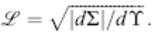
The absolute value in the definition (25) is necessary because the ray tube area dΣ changes sign upon every passage through a caustic. Every such passage gives rise to a non-geometrical, frequency-independent π/2 phase shift, or Hilbert transformation, of the associated wave. The Maslov index M is a monotonically increasing integer that keeps track of the number of caustic passages along a ray; the M-times-transformed pulse in (24) is
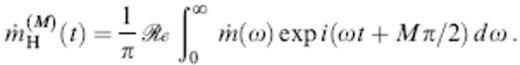
The first-arriving wave at every receiver r has M=0, so that the shape of the least-time pulse is always m˙H(0)(t)=m˙(t).
3.3 Ray-theoretical traveltime anomaly
The ‘exact’ ray-theoretical traveltime anomaly associated with the wave-speed perturbation δc is simply the difference in traveltime between s and r in the perturbed and unperturbed media,
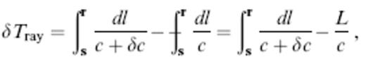
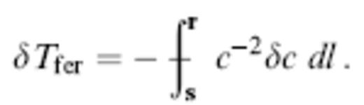
where the unadornment or adornment on an integral indicates that it is taken along the true geometrical (perturbed) or straight-ray (unperturbed) path. Fermat's principle can be used to linearize the relation (27); the traveltime anomaly is given in this approximation by a much simpler straight-ray integral:
The difference between δTray and δTfer is guaranteed to be of second order in the wave-speed perturbation:
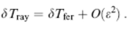
Fermat's principle is invoked in the vast majority of global traveltime tomographic studies, because it enables the inverse problem to be cast only in terms of integrals along the unperturbed spherical earth ray path, avoiding the need to perform 3-D ray tracing.
4 Banana–Doughnut Theory
Banana–doughnut theory accounts explicitly for the ability of a finite-frequency wave to ‘feel’ earth structure off the geometrical ray. The 1-D line integral (28) is replaced by a 3-D volume integral,

over the entire space,  , in which the wave-speed perturbation is non-zero, δc/c≠0. In Banana–;Doughnut I and II we used the Born approximation to find an ‘exact’ double-ray-sum representation of the 3-D Fréchet kernel in (30), and we have shown that this double-sum representation could be approximated very well by the leading term in a paraxial or near-ray expansion. We shall conduct all of our traveltime comparisons in this paper in terms of the paraxial rather than the ‘exact’ sensitivity kernel, because of the relative ease with which its generalization can be computed in a more realistic spherical background earth model.
4.1 Paraxial Fréchet kernel
We specify the location of a single-scatterer integration point x in eq. (30) in terms of the path-perpendicular ray-centred coordinates q1, q2 as well as the straight-ray distances L′ and L″=L−L′ to the source and receiver, as illustrated in Fig. 4. In the special case where the background medium is homogeneous, c=constant, the paraxial kernel K(x) is given by
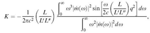
where q= is the perpendicular distance from the scattering point x to the nearest point on the straight source-to-receiver ray. The argument of the sinusoid in the uppermost integral is ω times the difference in traveltime ΔT=(1/2c) (L/L′L″)q2 required to take the detour path through the scatterer x rather than straight along the source-to-receiver ray. The identical dependence of this traveltime difference upon the two cross-path coordinates q1, q2 renders the straight-ray traveltime sensitivity kernel (31) axially symmetric. In addition, K exhibits a mirror-plane symmetry with respect to s and r, by virtue of the interchangeability of L′ and L″.
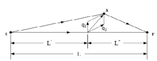
Geometrical notation used in the specification of the paraxial Fréchet kernel, eq. (31). Every single scatterer x is projected onto the nearest point on the straight-line source–receiver ray; the position of x relative to the projection point is described by the two orthogonal ray-centred coordinates q1, q2. The quantities L′ and L″=L−L′ are the distances from the projected point to the source s and receiver r, respectively.
The derivation of the result (30)–(31) in Banana–Doughnut I and II specifically assumes that the traveltime anomaly of a finite-frequency wave with power spectral density |m˙(ω)|2 has been measured by cross-correlation in the time domain, in accordance with the stipulation (19). In fact, eqs (30) and (31) can be regarded as the linearized version of eq. (19); i.e.,

in the same way that the Fermat approximation (28) is the linearization of (27).
4.2 Doughnut-hole geometry
Fig. 5 shows a cross-secal representation of the paraxial Fréchet kernel (31) for a τ=25 s wave observed at a source–receiver distance L=∥r−s∥=20λ. As noted in Banana–Doughnut I and II, the presence of the sinusoidal term sin(ωΔT) in the uppermost integral renders the sensitivity of a finite-frequency traveltime identically zero along the straight-line source–receiver ray, where q=0. The maximum sensitivity is in a dark-grey (K<0) ellipsoidal ‘banana skin’ surrounding the ray; the sensitivity is significantly reduced within the fringing light-grey (K>0) sidelobe and beyond as a result of destructive interference among adjacent frequencies ω and ω+dω in the waveform. Roughly speaking, the region of strong sensitivity lies within the first Fresnel zone, defined by ΩΔT≤π or, equivalently, ΔT≤τ/2. In our simple ellipsoidal geometry, this condition reduces to
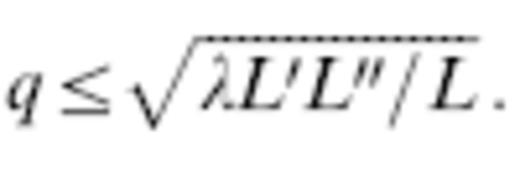
The cross-path width or diameter of the axially symmetric zone (33) at the source–receiver midpoint L′=L″=L/2 is  , as shown.

Axial cross-sec through the 3-D banana–doughnut traveltime sensitivity kernel K for an acoustic wave with a characteristic period τ=25 s, observed at a source–receiver distance L=20λ=4000 km. Note the scale: medium grey tone (background) represents K=0. Curve on right shows the cross-path variation of K versus q on a path-perpendicular plane midway between the source s and receiver r.
4.3 Fat man and little boy
Whenever the dimensions of an on-axis anomaly are large compared to the characteristic width of the kernel,
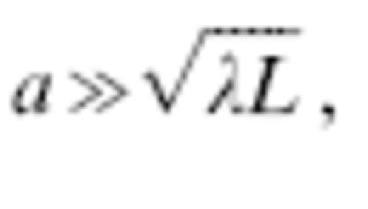
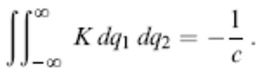
the wave-speed perturbation δc/c can be extracted from the 2-D integration over the transverse coordinates q1, q2 in eq. (30), leading to the approximation

The remaining integral over q1, q2 can be evaluated analytically, with the result
Upon inserting (36) into (35) we find that the traveltime anomaly reduces to that for an infinite-frequency wave:
This analysis shows that banana–doughnut theory provides the natural finite-frequency extension of linearized geometrical ray theory.
In the opposite limit of an on-axis perturbation that is small compared to the characteristic width of the kernel,
the traveltime anomaly (30) of a finite-frequency wave is negligible:
Such a small wave-speed anomaly is able to ‘hide’ inside the doughnut hole, where K≈0, as illustrated in Fig. 6. A large enough anomaly does not care if the 3-D Fréchet sensitivity kernel has a doughnut hole; the entire kernel then ‘sees’ essentially the same cross-path perturbation δc/c, so that δTbdk reduces to δTfer by virtue of the identity (36).
4.4 Wavefront healing mechanism
Fig. 7 illustrates the manner in which the 3-D Fréchet kernel (30)–(31) is able to account for finite-frequency, diffractive wavefront healing by virtue of the presence of the doughnut hole. In this schematic example, an anomaly of fixed size a=4λ is situated at fixed distance S=10λ from the source s. The top panel shows the kernel K for a receiver r at a distance R=2λ, corresponding to the point at which an infinite-frequency wave has just passed through the anomaly. The diameter of the anomaly is much greater than the local width of the kernel K, so that a finite-frequency wave will also accrue almost the full ray-theoretical advance or delay, δTbdk≈δTfer. The other two panels show the kernels K after the wave has propagated beyond the anomaly, to distances R=12λ and R=30λ, respectively. It is clear that the local width of the kernel K in the vicinity of the anomaly increases with the source–receiver distance, so that as the wave propagates, the anomaly finds itself increasingly able to ‘hide’ within the doughnut hole. In the limit R→∞ the anomaly will be 100 per cent successful in hiding, and the initial advance or delay will be completely eradicated by wavefront healing, δTbdk→0. We shall return to this hide-and-seek scenario in sec 6, in order to conduct a slightly more quantitative back-of-the-envelope analysis of this banana–doughnut mechanism of wavefront healing.
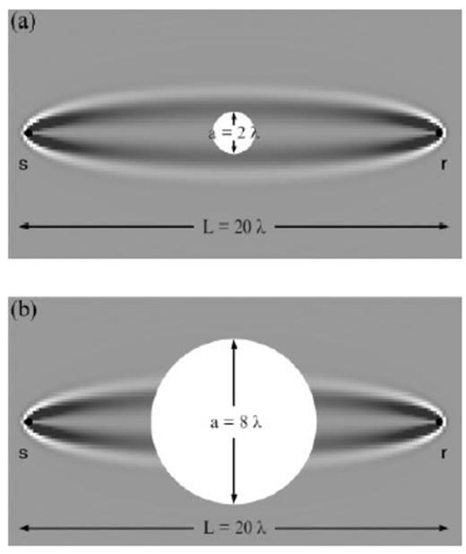
The cross-path width of an L=20λ Fréchet kernel K at the source–receiver midpoint L′=L″=L/2 is  . (a) A little-boy wave-speed anomaly of diameter a=2λ gives rise to a negligible traveltime shift, δTbdk≈0, because it is able to ‘hide’ within the doughnut hole. (b) A fat-man anomaly of diameter a=8λ appears to be uniform on the cross-path scale of the kernel; as a result, the traveltime shift is approximately that given by linearized ray theory, δTbdk≈δTfer.
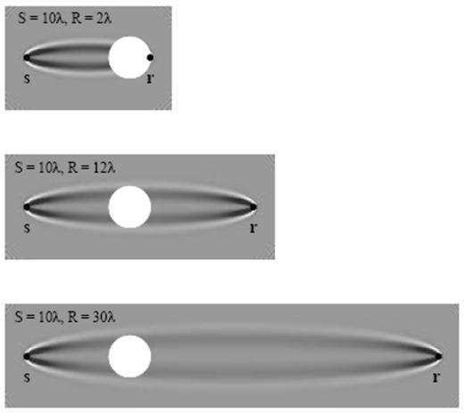
Schematic illustration of the banana–doughnut mechanism of wavefront healing. In this example, a wave-speed anomaly of diameter a=4λ is situated at a distance S=10λ from the source s. The three panels show the relation of the anomaly (white circle) to the 3-D traveltime sensitivity kernel K of a τ=25 s wave, as the position of the receiver r is shifted from R=2λ to R=12λ to R=30λ, representing the propagation of the wave. The size of the doughnut hole in the vicinity of the anomaly increases with increasing propagation distance, so that the traveltime shift δTbdk decreases with time.
5 Numerical Results
In this sec we test the linearity of ray theory by comparing δTfer with δTray and we examine the prediction capabilities of both linearized ray theory and banana–doughnut theory by comparing δTfer and δTbdk with ground truth cross-correlation traveltime anomalies δTccm for a variety of wave-speed anomaly magnitudes and source–receiver geometries. Many of the results we present here are reminiscent of those in the now classic study of Wielandt (1987). He studied the waveform and traveltime perturbations induced by a ‘hard’ spherical scatterer, with a constant wave-speed perturbation δc=constant, rather than a ‘soft’ scatterer, with a wave-speed perturbation (4) that blends smoothly into the background, as we do. We comment briefly upon another important difference between our study and that of Wielandt in sec 5.7.
5.1 Rays, wavefronts and caustics
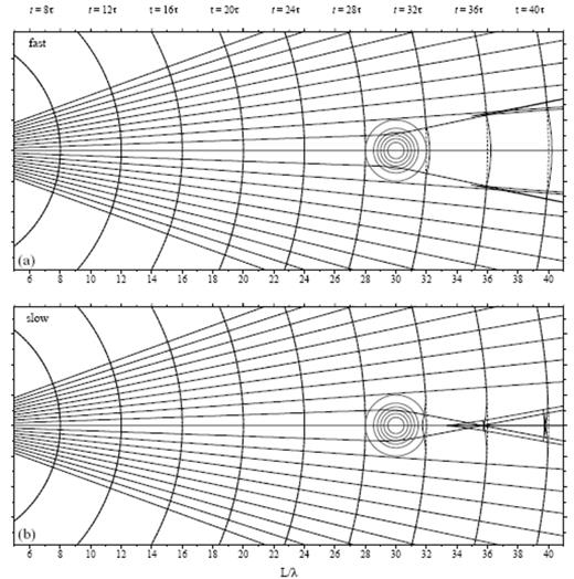
Fig. 8 presents a bare-bones ray-theoretical view of the wavefield passing through a fast anomaly (a) and a slow anomaly (b). Recall that each plot represents a 2-D cross-sec through an axially symmetric 3-D situation. The circular bull's-eyes on the left are contours of the wave-speed perturbation δc/c; the diameter in both cases is a=4λ and the anomaly magnitudes are ε=±6 per cent, corresponding to a straight-through Fermat traveltime advance or delay δTferφ=0=∓6 s, respectively. The diverging lines are geometrical rays emanating from a source s situated out of the picture at a distance S=10λ to the left. The curved solid lines are infinite-frequency wavefronts, which are everywhere perpendicular to the rays. Each vertical strip can be regarded as a snapshot of the propagating wave, taken at an instant t=8τ, 12τ,…, 40τ=200, 300,…, 1000 s given above. The dashed lines show the presence of the corresponding unperturbed spherical wavefront at the same instant; the advance of the wavefront upon passing through a fast (ε>0) anomaly and its delay upon passing through a slow (ε<0) anomaly are evident. The heavy solid lines are caustics, where the geometrical spreading factor ℒ in eqs (24) and (25) vanishes, because of the crossing of adjacent rays. A fast anomaly gives rise to a two-sheeted, funnel-shaped caustic, with a circular cusp at L≈17λ in 3-D space. The folding or triplication which the wavefront experiences upon passing through this cusp is too small to be seen at this scale. In the case of a slow anomaly, there are two caustics—a conical caustic with a pencil-point cusp at L≈14λ and a linear axial caustic that commences at this cusp. The conical caustic is associated with the crossing of rays that lie within the plane of the 2-D cross-sec shown. The triplication associated with this caustic is evident; note that the folds in the wavefront everywhere coincide with the caustic. The axial caustic is due to the crossing of adjacent rays that lie out of the 2-D plane. Beyond L≈14λ, all of the rays that leave the source at the same take-off azimuth φ cross the axis at the same point (see app for further details).
As usual, the ray-theoretical picture is extremely complicated, and marred by caustic singularities and triplicated wavefronts. Nevertheless, this example, makes one thing abundantly clear: wave propagation through a fast anomaly is decidedly different from propagation through a slow one. As we shall see, vestiges of this fast–slow asymmetry persist even for finite-frequency waves. There is no way that any strictly linear relationship such as (28) or (30) can capture this phenomenon. Evidently δTfer→−δTfer and δTbdk→−δTbdk whenever δc→−δc.
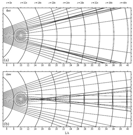
Axial cross-secs illustrating the passage of an infinite-frequency 3-D wavefield through a fast (a) and a slow (b) anomaly. Circular contours centred at L=10λ depict the cosine-bell wave-speed perturbation (4), of diameter a=4λ and maximum magnitude ε=±6 per cent. Thin solid lines are geometrical rays and wavefronts diverging from an S=10λ point source s (not shown). The corresponding unperturbed spherical wavefronts are depicted by dashed lines. Heavy solid lines are caustic singularities, where neighbouring rays cross. The triplications continue to expand laterally, and no additional caustics develop as the wavefront propagates further beyond the anomaly into homogeneous space. See Fig. 9 for corresponding finite-frequency view.
5.2 Finite-frequency waves
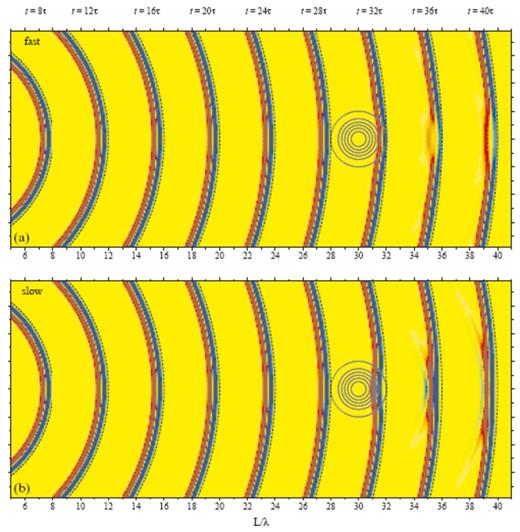
In Fig. 9 we see the wave-theoretical flesh grafted onto the ray-theoretical bones. The anomaly size a=4λ and magnitude ε=±6 per cent are unchanged, and the layout is analogous to that in Fig. 8; the upper and lower panels show the propagation of a τ=25 s wave through a fast and slow wave-speed perturbation, respectively. Each vertical strip represents a snapshot of the incremental pressure field phet(r, t) at time t=8τ,12τ,…,40τ; regions of compression (phet>0) and dilatation (phet<0) are designated by green–blue colours and orange–red colours, respectively. The reference locations of the unperturbed spherical wavefronts are shown by dashed lines, as before. Just after passing through the fast or slow anomaly, at time t=12τ=300 s, the leading green edge of the wavefront is visibly advanced (a) or delayed (b) with respect to the unperturbed wavefront. As time progresses, however, the extent of this advance or delay is diminished by diffractive processes; the sequence of snapshots provides a visualization of the wavefront healing phenomenon which is the principal focus of this paper.
The nature of the healing process is obviously quite different in the two examples. In the case of a fast anomaly, the on-axis (φ=0°) pulse amplitude diminishes with time, as a result of geometrical attenuation associated with the defocusing of rays in Fig. 8. It is also evident that the pulse width is substantially broadened; note the growing yellowish ‘lens’ between the leading blue compression and the trailing red rarefaction. In the case of a slow anomaly, the amplitude of the on-axis pulse is, in contrast, amplified by focusing and its width is narrowed. The only manifestation of the caustic singularities are weak orange and green diffractions, which lie along extrapolations of the folded infinite-frequency wavefronts (Fig. 9b). As usual, the exquisite detail in the infinite-frequency picture is blunted and blurred in the real finite-frequency world.
5.3 Source–receiver reciprocity
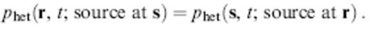
The principle of acoustic reciprocity guarantees that the pressure response to a pinpoint explosion m(t)δ(r−s) is invariant under an interchange r↔s of the source and receiver (Landau & Lifshitz 1959, sec 74):
We devote the present sec to a brief illustration of this fundamental result. Figs 10 and 11 show the rays, wavefronts and caustics and a sequence of snapshots of a τ=25 s pressure pulse phet(r, t) passing through a fast (a) and slow (b) a=4λ, ε=±6 per cent wave-speed anomaly. The formats of these figures are identical to those of Figs 8 and 9; the only difference is that the anomaly (bull's-eye) has been moved from S=10λ= 2000 km to a new position at a greater distance, S=30λ= 6000 km, from the source. All of the views prior to t=28τ=700 s are in this case quite boring; the rays are straight lines, the wavefronts are spherical, and the pressure response is simply that of a homogeneous medium, phet(r, t)=phom(r, t). The wavefront that finally encounters the anomaly is more nearly planar than that in Figs 8 and 9; as a result, the caustics and associated triplications develop more quickly, at distances L≈35λ and L≈33λ upon passage through a fast (Fig. 10a) and slow (Fig. 10b) anomaly, respectively. The blunted and blurred diffractions that are the finite-frequency manifestations of the ray-theoretical wavefront folding are evident in Fig. 11b.
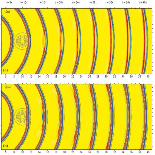
Axial cross-secs showing the passage of a finite-frequency (τ=25 s) acoustic pressure field phet(r, t) through a fast (a) and slow (b) a=4λ, ε=±6 per cent wave-speed anomaly. Green–blue colours denote regions of compression (phet>0); orange–red colours denote regions of dilatation or rarefaction (phet<0). Dashed lines show the reference location of the unperturbed spherical wavefront. See Fig. 8 for corresponding infinite-frequency, purely geometrical view.
The reciprocity principle (40) stipulates that the waveforms phet(r, t) should be identical at an on-axis (φ=0°) receiver situated at a distance L=40λ in the two cases S=10λ, R=30λ and S=30λ, R=10λ. It is clear that the blue → red → green patterns that are on the verge of passing through the φ=0° receiver are visually similar in the final t=40τ=1000 s snapshots in Figs 9 and 11. Note that there is no requirement that the responses phet(r, t) be identical anywhere other than at this S↔R receiver. In Fig. 12 we present a more quantitative vindication of eq. (40); the two panels show the synthetic fast-anomaly (Fig. 12a) and slow-anomaly (Fig. 12b) waveforms phet(r, t) at a sequence of on-axis (φ=0°) receivers, situated at distances L=8λ, 12λ,…, 40λ. Solid and dashed lines depict the responses for the near-source (S=10λ) and the more distant (S=30λ) anomalies, respectively; the amplitude of each pulse has been scaled by a factor proportional to the propagation distance L, in order to eliminate the effect of L−1 geometrical spreading in the background model. At distances L≤8λ all four pulses phet(r, t;ε>0 or ε<0; S=10λ or S=30λ) are identical, and simply equal to phom(r, t), because none of the waves has yet encountered an anomaly. Between L=8λ and L=28λ the perturbed S=10λ waveforms phet(r, t) are very clearly advanced (ε>0, top) or delayed (ε<0, bottom) in time relative to the unperturbed S=30λ waveforms phet(r, t)=phom(r, t). At L=12λ, immediately after the waves have passed through the S=10λ anomaly, the extent of this visual traveltime shift is approximately equal to the expected ray-theoretical advance or delay, δTferφ=0=∓6 s. With increasing propagation distance, however, the visual traveltime shift decreases by a factor of two to three, as a consequence of diffractive wavefront healing. The geometrical attenuation of phet(r, t) relative to phom(r, t) due to ray defocusing upon passage through a fast anomaly and its relative amplification due to focusing upon passage through a slow anomaly are also evident. At L=32λ the S=30λ pressure pulses phet(r, t) have just passed through the anomalies, where they accrue their ray-theoretical traveltime shifts δTferφ=0=∓6 s. These shifts and the attendant defocusing (top) and focusing (bottom) reduce the discrepancy between phet(r,t;S=10λ) and phet(r,t;S=30λ). The discrepancy continues to decrease with increasing propagation distance until, finally, at L=40λ, the two pulses merge and become identical, in accordance with the principle of acoustic reciprocity (40). The visual indistinguishability of the solid and dashed waveforms phet(r,t;S=10λ, R=30λ) and phet(r,t;S=30λ, R=10λ) is indicative of the accuracy of the numerical procedure used to solve eqs (7) and (8).
Same as Fig. 8, except that the anomaly (bull's-eye) is situated at a distance S=30λ from the source s. Prior to t=28τ=700 s, the geometrical rays are straight and the perturbed (solid) and unperturbed (dashed) wavefronts coincide, because the spherically symmetrical waves are simply propagating through a homogeneous medium. See Fig. 11 for corresponding finite-frequency view.
5.4 Traveltime comparisons
Fig. 13 illustrates the cross-correlation traveltime measurement process for an on-axis (φ=0°) suite of synthetic pressure-response seismograms at various distances 2λ≤R≤30λ beyond a fast (Fig. 13a) or slow (Fig. 13b) anomaly. The anomaly location S=10λ and diameter a=4λ are the same as those in Figs 8 and 9; however, the magnitude of the wave-speed perturbation is half as large, ε=±3 per cent. Solid lines are used to display the perturbed waveforms phet(r, t) in the plots on both the left and right; dashed lines on the left depict phom(r, t), whereas those on the right depict the corresponding optimally aligned, unperturbed waveforms phet(r, t−δTccmφ=0). Immediately after passage through the anomalies, at R=2λ, the unperturbed pulses are advanced (Fig. 13a) or delayed (Fig. 13b) with respect to the unperturbed pulses by roughly the full ray-theoretical amount, δTccmφ=0≈δTferφ=0=∓3 s. Once the pulses have propagated to the most distant, R=30λ, receivers, however, diffractive wavefront healing has reduced the cross-correlation traveltime δTccmφ=0 by a factor of 70–80 per cent. It is noteworthy that the degree of healing, as measured by cross-correlation, is somewhat more pronounced for the fast anomaly than for the slow one; this fast–slow asymmetry is a general feature, which becomes more pronounced when the absolute magnitude |ε| of the wave-speed perturbation increases, as we shall see in sec 5.6.
In Fig. 14 we conduct a more thorough analysis of the source-anomaly configuration in Fig. 13, examining all four quantitative measures (19), (27), (28) and (30) of δT over the full range of receiver azimuths, −45°≤φ≤45°, at three different source–receiver distances L=12λ (Fig. 14a), L=22λ (Fig. 14b) and L=40λ (Fig. 14c). The top two panels compare the linearized Fermat anomaly δTfer (dashed line) with the ‘exact’ ray-theoretical anomaly δTray (solid line). The cusp of the slow anomaly lies immediately in front of the most distant, L=40λ, receiver, and one can just see a tiny triplication starting to form. All of the receivers lie in front of the caustic in the case of a fast anomaly. Note that δTfer need not coincide with, and in fact can be either greater or less than, δTray even along the straight-through (φ=0°) ray. The least-time character of the first-arriving waves does not dictate that δTray≤δTfer whenever the linearization (28) is performed in terms of the wave speed rather than the associated slowness perturbation, as we have done.
In the bottom two panels (Figs 14c and d) we test the extent to which banana–doughnut theory is able to reproduce ground truth cross-correlation traveltime measurements. The predicted and measured anomalies δTbdk and δTccm are denoted by filled circles and unfilled triangles, respectively. The dashed lines, which are identical to those in the top two panels, show the Fermat anomalies δTfer for comparison. It is evident that the 3-D Fréchet kernels (31) are able to account reasonably well for the healing of the finite-frequency traveltimes in this example. In general, the discrepancy between δTbdk and the measurements δTccm is about the same as or less than that between δTfer and δTray, due to the linearization of ray theory. Particularly at the largest propagation distance, L=40λ, the difference between δTbdk and δTccm is more pronounced for the fast anomaly than for the slow one. Since δTfer does not account for finite-frequency wavefront healing at all, it is in very poor agreement with the cross-correlation measurements δTccm, except at the L=12λ receivers situated just behind the anomaly.
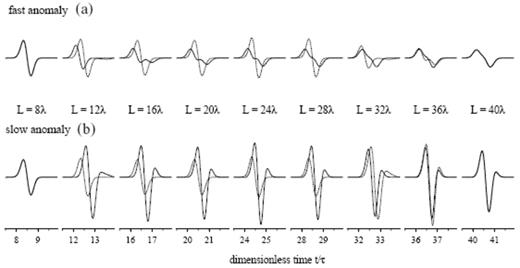
Synthetic pseudospectral seismograms phet(r, t) at a number of on-axis receivers r, situated at distances L=8λ, 12λ,…, 40λ from the source. Solid and dashed lines depict the waveforms for the S=10λ and S=30λ wave-speed anomalies illustrated in Figs 8–9 and 10–11, respectively. (a) phet(r, t) for an a=4λ, ε=+6 per cent fast anomaly, (b) phet(r, t) for an a=4λ, ε=−6 per cent slow anomaly; ticks on horizontal axis denote time t since detonation of the source, measured in integral multiples of the characteristic wave period τ. All pulse amplitudes have been corrected for the L−1 effect of background geometrical spreading. The indistinguishability of the solid and dashed L=40λ waveforms (far right) is guaranteed by the principle of acoustic source–receiver reciprocity, eq. (40).
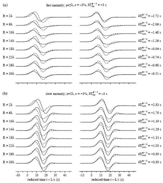
Perturbed and unperturbed waveforms at various distances R=2λ, 6λ,…, 30λ behind (a) an a=2λ, ε=−3 per cent and (b) an a=2λ, ε=+3 per cent anomaly. Solid lines on both left and right denote phet(r, t); dashed lines denote phom(r, t) before shifting (left) and phom(r, t−δTccmφ=0) after shifting (right) to maximize cross-correlation (19). The measured traveltime shift δTccmφ=0 is indicated in each case. All pulse amplitudes have been scaled by a factor proportional to L, to eliminate the effect of background geometrical spreading. The relative attenuation of the perturbed pulse due to defocusing behind a fast anomaly (a) and its amplification due to focusing behind a slow anomaly (b) are again apparent. Note that the horizontal timescale has been reduced by the background wave speed, c=8 km s−1; this choice aligns all of the unperturbed pulses phom(r, t).
5.5 Effect of anomaly size
In Fig. 15 we examine the effect of the physical size of the anomaly upon the waveforms at a fixed source–receiver distance L=22λ, but at various azimuths 0°≤φ≤45°. The solid lines in the left (Fig. 15a), middle (Fig. 15b) and right (Fig. 15c) columns show phet(r, t) for a slow anomaly with dimensions a=2λ, a=4λ and a=8λ, respectively; the dashed lines show the corresponding unperturbed, unshifted waveforms phom(r, t) for comparison. Each of the anomalies has been scaled to give the same straight-through Fermat delay, δTferφ=0=+6 s; the resulting wave-speed perturbations are ε=−12 per cent, ε=−6 per cent and ε=−3 per cent. The parameters in Fig. 15(b) are identical to those in Figs 8 and 9. Regardless of the size of the anomaly, the waveforms are very little perturbed at azimuths in excess of φ=20°–30°; the anomaly is then too far off the source–receiver axis to be significantly ‘felt’ by the waves. It is evident that a large, a=8λ, slow wave-speed anomaly gives rise to very nearly the full 6 s, φ=0° ray-theoretical delay, δTvisφ=0≈δTferφ=0; on the other hand, a small, a=2λ, slow anomaly produces very little visible delay in the arrival of the on-axis pulse, δTvisφ=0≈0. This is the expected consequence of the fat-man, little-boy distinction depicted in Fig. 6.
Fig. 16 compares the various measures of the traveltime shift for both fast and slow δTferφ=0=∓6 s anomalies of small (a=2λ, ε=±12 per cent), intermediate (a=4λ, ε=±6 per cent) and large (a=8λ, ε=±3 per cent) size. The source–receiver distance in all six cases is L=22λ, as before. The dashed line in every plot is the linear Fermat traveltime anomaly δTfer. The azimuthal range subtended by the anomaly increases from approximately −10°≤φ≤10° to −30°≤φ≤30° as the size increases from a=2λ to a=8λ. The solid line in the top two panels is the exact ray-theoretical traveltime anomaly δTray. Both an a=2λ and an a=4λ fast anomaly produce a flank triplication with its ‘crossover point’ at φ≈±10°; recall that the solid line is a cross-sec of a 3-D, axially symmetric wavefront. Likewise, there is an axially symmetric triplication with its ‘crossover point’ at φ=0° in the case of both an a=2λ and an a=4λ slow anomaly. The fast wavefronts can loosely be thought of as propagating upwards and the slow wavefronts as propagating downwards.
The unfilled triangles and filled circles in the two lower panels of Fig. 16 denote the measured cross-correlation traveltime anomalies δTccm and the banana–doughnut traveltime anomalies δTbdk, respectively. Banana–doughnut theory reduces to linearized ray theory in the case of an a=8λ fat-man anomaly, and either theory is capable of modelling the ground truth measured traveltime shifts, δTbdk≈δTfer≈δTccm. Finite-frequency diffraction effects have healed the on-axis measurements δTccmφ=0 by approximately 50 per cent in the case of an intermediate-sized a=4λ anomaly; however, this healing is well described by the banana–doughnut Fréchet kernels for both the fast and slow anomaly. The healing is much more significant, virtually 100 per cent, for an a=2λ little-boy anomaly; banana–doughnut theory is not quite as successful in this case, but it is certainly far superior to linearized ray theory. Once again, we see that the discrepancy between δTbdk and δTccm is somewhat more pronounced for a fast than for a slow anomaly.
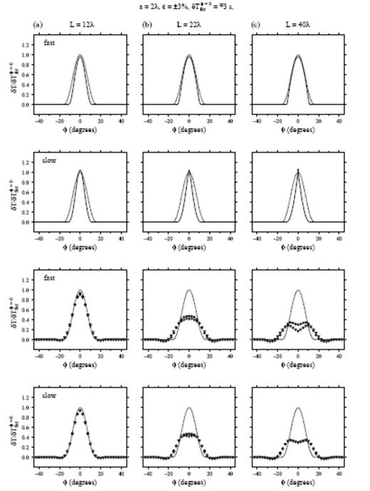
Comparison of both ray-theoretical and banana–doughnut predictions with ground truth, cross-correlation traveltime-shift measurements at three source–receiver distances (a) L=12λ, (b) L=22λ and (c) L=40λ, following passage through an S=10λ, a=4λ, ε=±3 per cent fast or slow wave-speed anomaly. Solid lines in top two panels show the ‘exact’ ray-theoretical traveltime shifts δTray; filled circles and unfilled triangles in bottom two panels denote the banana–doughnut traveltime shifts δTbdk and the cross-correlation measurements δTccm, respectively. Dashed lines in all plots show the linearized Fermat anomalies δTfer for comparison. Vertical axis is the normalized traveltime shift δT/δTferφ=0 in all plots. See Fig. 13 for a depiction of the perturbed and unperturbed waveforms phet(r, t) and phom(r, t).
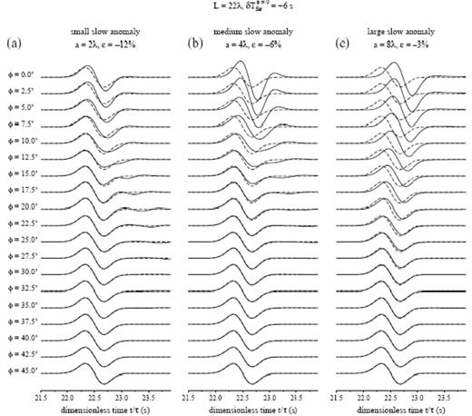
Synthetic pressure-response seismograms at a fixed source–receiver distance L=22λ, following passage through (a) a small, (b) a medium and (c) a large slow wave-speed anomaly situated at a distance S=10λ from the source. The straight-through Fermat delay is the same, δTferφ=0=+6 s, in all three cases. Solid and dashed lines denote the perturbed and unperturbed waveforms phet(r, t) and phom(r, t), respectively. Receiver azimuth 0°≤φ≤45° is indicated on the extreme left. Horizontal axis is dimensionless time t/τ since detonation of source.
5.6 On-axis healing
In Fig. 17 we specifically examine healing along the φ=0° axis immediately behind an intermediate-sized, a=4λ, anomaly. The vertical axis in the plot on the left (Fig. 17a) is the measured cross-correlation traveltime anomaly δTccmφ=0; the corresponding prediction δTbdkφ=0 of banana–doughnut theory is shown on the right (Fig. 17b). The horizontal axis in both cases is the magnitude of the anomaly, ε=±3, 4, 5, 6 per cent. The ∼45° solid lines show the infinite-frequency Fermat anomaly, which obviously depends linearly upon the anomaly magnitude, reaching δTferφ=0=∓6 s for ε=±6 per cent, respectively. The circles, diamonds, triangles and squares show the measured and predicted anomalies δTccmφ=0 and δTbdkφ=0 at the four downstream distances R=3λ, 6λ, 15λ and 27λ, respectively. The extent to which these points lie between the ∼45° line and the horizontal axis is a measure of the percentage healing. If banana–doughnut theory provided a perfect description of wavefront healing, then Fig. 17(b) would look identical to Fig. 17(a). This is very nearly so at all distances for a slow (ε<0) anomaly, as well as at the closest receivers (R=3λ, 6λ, 15λ) behind a fast (ε>0) anomaly. The largest discrepancy between δTbdkφ=0 and δTccmφ=0 is at the most distant (R=27λ) receiver behind a fast anomaly.
We examine the reason for this marked long-distance fast–slow asymmetry in Fig. 18. The top two plots compare the healing behaviour at various distances 0≤R≤30λ behind an a=4λ, ε=+6 per cent (Fig. 18a) and an a=4λ, ε=−6 per cent (Fig. 18b) anomaly. The measured traveltimes δTccmφ=0 behind the slow (ε<0) anomaly are well behaved and well modelled at all distances by the banana–doughnut predictions δTbdkφ=0. Behind the fast (ε>0) anomaly, however, the measurements δTccm are more scattered, and appear to undergo a transition to a much stronger healing regime at R≈15λ. This behaviour is symptomatic of the competition between two distinct contributions to the cross-correlated waveform—a defocused and therefore low-amplitude first arrival that is advanced because it has passed straight through the fast anomaly and a later-arriving diffraction that has ‘crept’ around the centre of the ‘soft’ anomaly. The presence of this diffracted arrival is distinctly visible in the nascent ‘double-bump’ waveform phet(r, t) at the most distant, R=30λ, receiver. In essence, a cross-correlation traveltime measurement based upon the minimization (19) fits the second ‘bump’ rather than the first, resulting in a measured traveltime shift, δTccmφ=0/δTferφ=0=(0.69 s)/(−6 s)≈−0.1, that appears to be ‘overhealed’. The measurements behind a slow anomaly are much less affected by any comparable later-arriving diffraction, because the first arrival is delayed and geometrically amplified by focusing, rather than being advanced and geometrically attenuated. The resulting R=30λ waveform shows no evidence of a ‘double bump’, and the minimization procedure (19) is able to ‘lock’ successfully onto the desired first arrival.
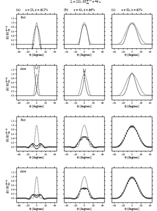
Same as Fig. 14, except that all of the traveltime shift measurements have been made at the same source–receiver distance L=22λ, following passage of a wave through (a) a small, (b) a medium (c) and a large δTferφ=0=+6 s slow S=10λ anomaly. Vertical axis is the normalized traveltime shift δT/δTferφ=0 in all plots. See Fig. 15 for a depiction of the perturbed and unperturbed waveforms phet(r, t) and phom(r, t).
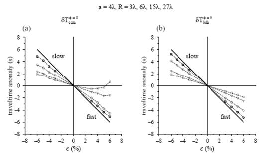
On-axis (φ=0°) traveltime shifts following passage of a τ=25 s wave through an a=4λ anomaly of varying magnitude, ε=±3, 4, 5, 6 per cent, situated at a distance S=10λ from the source. Side-by-side plots display (a) the cross-correlation traveltime shift δTccmφ=0 and (b) the banana–doughnut traveltime shift δTbdkφ=0 at four different distances, R=3λ (circles), R=6λ (triangles), R=15λ (diamonds), R=27λ (squares) behind the anomaly. The unhealed Fermat anomaly δTferφ=0 is indicated by the ∼45° solid line in both plots.
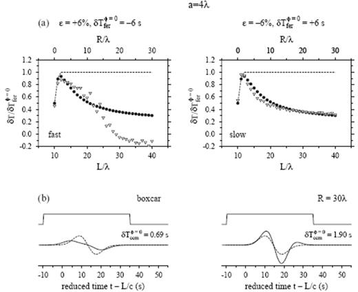
(a) Top two plots illustrate the evolution of δTbdkφ=0 (filled circles), δTccmφ=0 (unfilled triangles) and δTferφ=0 (dashed line), following the propagation of a τ=25 s wave through a fast (left) and slow (right) S=10λ, a=4λ, ε=±6 per cent wave-speed anomaly. Vertical axis is the normalized traveltime shift δT/δTferφ=0 in all plots. The L=10λ receiver is located at the centre of the anomaly; the full Fermat advance or delay δTferφ=0=∓6 s is not attained until L=12λ, where the waves have passed completely through. (b) Solid and dashed lines in the bottom two plots display the perturbed and the shifted, unperturbed waveforms phet(r, t;R=30λ) and phom(r, t−δTccmφ=0; R=30λ), respectively; overlying boxcars show the t2−t1=45 s time window used in the cross-correlation traveltime measurement (19). Horizontal axis is reduced time, t−L/c. The fast-anomaly measurements δTccmφ=0 begin to diverge markedly from the banana–doughnut predictions δTbdkφ=0 at R≈15λ, due to the increasing importance of diffracted waves that ‘creep’ at the background speed, c=8 km s−1, around the centre of the 3-D inclusion.
In Fig. 19 we show that it is possible to improve the agreement between δTbdkφ=0 and δTccmφ=0 behind a fast anomaly by introducing a forward-weighted taper w(t) into the cross-correlation, replacing the criterion (19) by
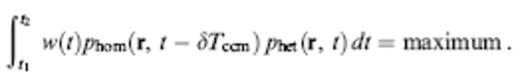
The adoption of a one-sided 60 per cent cosine taper w(t) with a total length t2−t1=35 s results in a series of measurements δTccm that are tolerably close to the banana–doughnut predictions δTbdk at all distances 0≤R≤30λ behind both a fast and slow S=10λ anomaly, as shown. Not surprisingly, however, the measurements are rather sensitive to the overall length and detailed shape of the taper. It would obviously be rash, on the basis of this single, highly idealized, synthetic experiment, to advocate the real-world application of forward-weighted tapers in automated cross-correlation traveltime measurement schemes. We shall briefly discuss the results of using a battle-tested, interactive method for preferentially weighting the initial onset of phet(r, t) in sec 7.
5.7 Comparison with previous results
The on-axis healing patterns exhibited by the untapered traveltime shifts δTccm in Fig. 18 are in broad agreement with the theoretical evolution curves for the group delay of a monochromatic Gaussian beam derived by Nolet & Dahlen (2000). In both analyses, a fast traveltime shift initially heals slightly more slowly than a slow shift does; beyond a critical distance, however, the healing of a fast shift overtakes that of a slow shift, eventually even ‘overhealing’, so that δTccmφ=0/δTferφ=0<0. In contrast, Wielandt (1987) found very little healing in the wake of a fast ‘hard’ spherical scatterer, even at dimensionless propagation distances R/λ much greater than those considered in the present ‘soft’ scatterer study. The cause of this significantly different behaviour is that Wielandt (1987) used an automated picking algorithm to measure the onset time of the first arriving wave. In the case of a positive wave-speed perturbation, δc/c>0, the first arrival may be significantly reduced in amplitude as a result of defocusing, but it always arrives before the corresponding unperturbed spherical wave in a homogeneous background medium, because it has passed straight through the anomaly rather than creeping around it. In practice, the onset of a broad-band body-wave pulse is difficult to determine in the presence of seismic noise; this is the principal reason for the popularity in global seismology of the cross-correlation traveltime shift measurements studied here.
Same as Fig. 18 except that a 60 per cent cosine taper w(t) of total duration t2−t1=35 s has been used to weight preferentially the early-arriving portions of the perturbed and the shifted, unperturbed waveforms phet(r, t) and phom(r, t−δTccmφ=0) in eq. (41). Horizontal axis in bottom two plots is reduced time, t−L/c. The resulting R=30λ traveltime measurements δTccmφ=0=−2.34 s (fast anomaly, left) and δTccmφ=0=+2.19 s (slow anomaly, right) are in much better agreement with the predictions δTbdkφ=0 of banana–doughnut theory.
5.8 Banana–doughnut versus ray theory
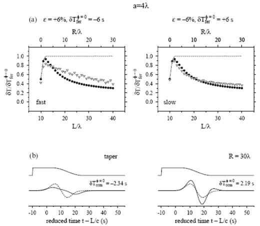
We present a summary assessment of the validity of banana–doughnut theory in our highly simplified study of 3-D wavefront healing in Fig. 20. As a measure of goodness we use the absolute (L1 norm) discrepancy between the predicted and ground truth traveltime shifts at all of the on-axis (φ=0°), post-anomaly (S=10λ, 0≤R≤30λ) receivers:
(a) and (b) Average L1 discrepancy Ebdk and (c) and (d) Efer at all of the on-axis (φ=0°) receivers, behind a number of different fast (left) and slow (right) wave-speed anomalies. The source anomaly distance is fixed at S=10λ; the entire suite of post-anomaly receivers 0≤R≤30λ is included in the misfit sums (42) and (42). Horizontal axes of each perspective 3-D box plot are the dimensionless radius a/λ and the magnitude ε of the perturbation; contours on floor give the corresponding straight-through Fermat anomaly δTferφ=0. Note the fivefold difference in vertical scales: 0≤Ebdk≤20 per cent (top) whereas 0≤Efer≤100 per cent (bottom).
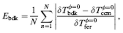
where δTccmφ=0 is measured using an untapered cross-correlation (19) rather than (41), and N is the total number of receivers r in the sum. The top two diagrams plot this untapered banana–doughnut misfit factor Ebdk as a function of the size λ≤a≤8λ and magnitude 3 per cent≤|ε|≤12 per cent of a fast (Fig. 20a) and slow (Fig. 20b) anomaly. The hyperboloids on the floors of the cubes are contours of the straight-through Fermat traveltime anomaly δTferφ=0, which is used as a normalizing factor in the denominator of the banana–doughnut misfit definition (42). The corresponding absolute ray-theoretical misfits,
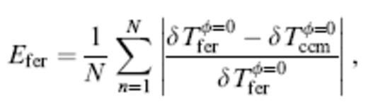
are plotted in the two bottom diagrams (Fig. 20c and d), for comparison. All of the wavefront healing trends which we have identified previously are evident in the misfit comparisons:
(i)Banana–doughnut theory (30) analytically reduces to linearized ray theory (28), and both theories are in good agreement with measured cross-correlation traveltime shifts, δTbdk≈δTfer≈δTccm, in the limit of a sufficiently large anomaly, a≥6λ–8λ.
(ii)In general, the discrepancy between δTbdk and δTccm is larger for wave-speed anomalies with a larger absolute Fermat traveltime shift |δTfer|.
(iii)The discrepancy is slightly larger for fast anomalies than it is for slow ones. As we have seen, this deficiency is the result of a fundamental fast-slow asymmetry in the healing process, which cannot be accounted for by any linearized relationship, and which manifests itself most strongly at long propagation distances.
(iv)Finally, and most importantly, banana–doughnut traveltime predictions δTbdk are consistently better than linearized ray-theoretical predictions δTfer, particularly for small anomalies, a=λ–4λ, with large wave-speed perturbations, |ε|=6–12 per cent. Typically, the agreement with measured cross-correlation traveltimes δTccm is improved by a factor of five to 10, that is Ebdk≈(0.1– 0.2)×Efer.
6 Cramming a Ball Into a Banana
Roughly speaking, the criterion for the validity or invalidity of linearized ray theory is whether a≫ or a≪
or a≪ , as we have seen in sec 4.3. In this sec, we shall improve upon this imprecise criterion slightly, by conducting an elementary geometrical analysis of the ability of an anomaly to ‘hide’ itself inside a banana–doughnut hole. Specifically, the quantity we seek to estimate is the percentage amount by which an on-axis Fermat traveltime anomaly has been healed:
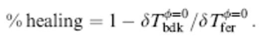
Both Tbdkφ=0 and δTferφ=0 depend linearly upon the wave-speed perturbation δc, so that the banana–doughnut prediction of the percentage healing (44) depends only upon the three purely geometrical dimensionless parameters a/λ, S/λ and R/λ, and is independent of the sign and magnitude of the per cent perturbation ε.
Figs 21(a) and (b) illustrate the banana–doughnut percentage healing (44) behind an a=4λ anomaly situated at a distance S=10λ (Fig. 21a) and S=30λ (Fig. 21b) behind the source. The evolution of δTbdkφ=0/δTferφ=0 behind the S=10λ anomaly is identical to that shown by the solid circles in Figs 18 and 19; at a distance R=30λ the healing amounts to 70 per cent. Because the impinging wavefronts are more nearly planar, the healing occurs slightly more rapidly behind the S=30λ anomaly; in this case 70 per cent healing is attained at a distance R=10λ. The symmetrical dependence of (44) upon S/λ and R/λ is of course a consequence of source–receiver reciprocity.
To begin our simplistic banana-cramming analysis, we note that the cross-secal area of the first Fresnel zone of a 3-D traveltime Fréchet kernel (31) at the centre of an on-axis anomaly is
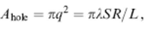
where we have substituted L′=S and L″=R in eq. (33) to obtain the second equality. A fast or slow anomaly of diameter a and cross-secal area
will be unable or able to ‘hide’ in the hole (45) depending upon whether Aanom≫Ahole or Ahole≪Aanom. The healing will be total if the anomaly is completely hidden, so we expect the percentage healing to be given approximately by

where the constant is introduced to account for the details of the overlap between the outer portions of the wave-speed perturbation δc/c and the inner regions of the doughnut hole in the 3-D integration (30). Empirically, we find that a suitable value for this overlap ‘fudge factor’ is const=1/4. With this choice, eq. (47) can be rewritten in terms of the non-dimensional distances a/λ, S/λ and R/λ in the form
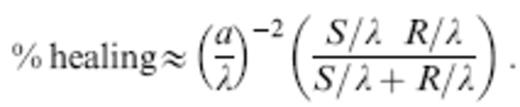
As anticipated, the approximate degree of healing (48) is invariant under an interchange S↔R of the distance of the anomaly to the source and receiver; the maximum healing occurs when an anomaly of a given size a is situated at the source–receiver midpoint S=R=L/2, where the banana–doughnut kernel K is the fattest.
Fig. 21(c) compares the approximate relation (48) with the ‘exact’ banana–doughnut healing percentage (44), for source–receiver configurations satisfying S=R=40λ, 0≤S, R≤40λ, and anomalies of various sizes 3λ≤a≤8λ. The agreement is obviously far from perfect; nevertheless, it is clear that (48) can be used to provide a back-of-the-envelope estimate, accurate to within ±20 per cent, of the degree of wavefront healing following propagation through a quasi-spherical wave-speed anomaly. In any more realistic spherical-earth application, the wavelength λ should be that at the depth of the anomaly, and the distances S and R should be measured along the unperturbed source–receiver ray.
To give a concrete example, a τ=20–25 s shear wave, with a wavelength λ≈150 km will, according to eq. (48), have healed by almost 50 per cent upon passage through an anomaly of diameter a≈700 km situated at the midpoint, R≈S≈4000 km, of the associated turning ray. A τ≈1 s compressional wave, with a wavelength λ≈13 km, will, on the other hand, heal by a negligible amount, less than 4 per cent, upon passage through the same size anomaly. This example shows that linearized ray theory (28) can reliably be used to resolve 700 km wave-speed variations in any inversion study based solely upon ISC compressional-wave traveltime data. Naive reliance upon ray theory to invert cross-correlation traveltimes of 20–25 s shear waves will, in contrast, result in a severe underestimation of the magnitude of 700 km anomalies. Banana–doughnut Fréchet kernels provide a proper theoretical basis for traveltime inversions that utilize such long-period, long-wavelength waves.
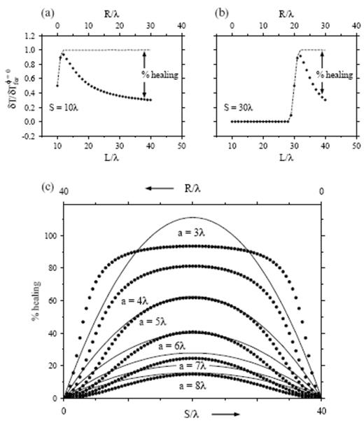
Pictorial definition of the per cent healing (44) behind (a) an a=4λ, S=10λ and (b) an a=4λ, S=30λ anomaly. Filled circles and dashed lines denote banana–doughnut and Fermat traveltime shifts δTbdkφ=0 and δTferφ=0, respectively. (c) Filled circles and solid lines denote ‘exact’ and approximate banana–doughnut healing percentages (44) and (47), respectively, for a range of anomaly diameters 3λ≤a≤8λ. Source-receiver distance is fixed, L=40λ; source–anomaly and receiver-distances vary from S=0, R=40λ (left) to S=40λ, R=0 (right). Both the ‘exact’ and approximate healing percentages are symmetrical about the source–receiver midpoint S=R=20λ.
7 Scripps Picks
We noted in sec 5.6 that it is possible to improve the agreement between δTbdk and δTccm by emphasizing the initial portions of the perturbed pressure pulse in the cross-correlation measurement procedure. In fact, such a ‘fit the first swing’ philosophy has long guided the global traveltime measurement programme conducted by researchers at the Scripps Institution of Oceanography (Masters et al. 1996). In their interactive procedure, an observed and a spherical-earth pulse are first rescaled to have the same maximum amplitude; the two pulses are then displayed on a workstation screen, and the synthetic is click-shifted until the initial up-or-down swings are aligned to the subjective satisfaction of the analyst. We report in this sec the results of a modest experiment, in which we use the Scripps software to process a handful of our ground truth pseudospectral waveforms phet(r, t) and phom(r, t).
The measurement technique is illustrated in Fig. 22. The top two traces (Fig. 22a) show the perturbed (solid line) and unperturbed (dashed line) synthetic seismograms at a distance R=30λ behind a fast and slow a=4λ, ε=±3 per cent anomaly. A slight advance (left) or delay (right) of phet(r, t) relative to phom(r, t) is evident; however, it is obvious that these shifts are less than the straight-through Fermat advance or delay δTferφ=0=∓3 s, as a result of finite-frequency wavefront healing. Straightforward application of our usual automated cross-correlation measurement procedure (19) leads to the best-fit alignments shown in the middle two traces (Fig. 22b). The measured traveltime shifts are
In the Scripps procedure phet(r, t) and phom(r, t) are rescaled and the initial upswings are interactively aligned, as shown in the bottom two traces (Fig. 22c). This results in significantly different traveltimes, namely,
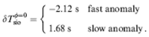
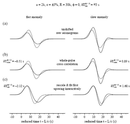
Comparison of ‘whole-pulse’ cross-correlation and Scripps interactive traveltime measurement procedures. Solid and dashed lines display perturbed and unperturbed waveforms, respectively. The centre of the anomaly is situated at a distance S=10λ from the source. (a) Raw seismograms phet(r, t) and phom(r, t) at an on-axis (φ=0°) receiver, situated at a distance R=30λ behind an a=2λ, ε=+3 per cent anomaly (left) and an a=2λ, ε=−3 per cent (right) anomaly. (b) Best-fit alignment of phet(r, t) and phom(r, t−δTccmφ=0), as determined by automated cross-correlation (19). (c) Interactive alignment of the initial upswings of phet(r, t) and phom(r, t−δTsioφ=0). The Scripps ‘initial-swing’ traveltime shifts δTsioφ=0 are significantly less healed than the automated ‘whole-pulse’ shifts δTccmφ=0.
Clearly δTsioφ=0 is much closer to δTferφ=0 than δTccmφ=0 is. Fitting the first upswing or downswing appears to emphasize the higher-frequency components of the pulse, thereby reducing the effects of wavefront healing.
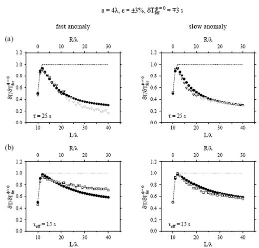
Fig. 23 shows the results of a more comprehensive comparison, for the same a=4λ, ε=±3 per cent fast (left) and slow (right) anomaly. The unfilled triangles and squares in the top (Fig. 23a) and bottom (Fig. 23b) panels represent the automated ‘whole-pulse’ and Scripps ‘initial-swing’ traveltime-shift measurements δTccmφ=0 and δTsioφ=0, respectively. The unhealed Fermat anomalies δTferφ=0=∓3 s are displayed as dashed lines, for comparison. The filled circles in the top panel are the banana–doughnut predictions δTbdkφ=0, for a wave with the actual characteristic period τ=25 s, whereas those in the bottom panel are the predictions δTbdkφ=0 for a slenderized banana–doughnut Fréchet kernel Keff, computed using eqs (13) and (31), with τ replaced by an effective period,
The cross-path width of Keff is less than that of the actual Fréchet kernel K by a factor of only  per cent. As we have seen, however, the degree of healing (47–48) depends to a good approximation upon the cross-secal area of the doughnut hole, so it is reduced by the square of this factor, 15/25=60 per cent.
The value of the effective period (51) was chosen by trial and error to provide a reasonably good agreement between the banana–doughnut predictions δTbdkφ=0 and the Scripps measurements δTsioφ=0 over a wide range of fast and slow anomaly magnitudes ε=±3, 4, 5, 6 per cent. This is illustrated in Fig. 24, which is plotted using a format identical to that in Fig. 17. In this case the circles, diamonds, triangles and squares show the measured and predicted anomalies δTsioφ=0 (τ=25 s) and δTbdkφ=0 (τeff=15 s) at the same four distances R=3λ, 6λ, 15λ and 27λ behind the anomaly. The strong similarity between Fig. 24(a) and Fig. 24(b) indicates that the degree of wavefront healing experienced by the initial upswing or downswing of a τ=25 s pulse is well modelled by an artificially emaciated banana–doughnut kernel Keff, with an effective period τeff=15 s. As usual, the agreement is better for the slow anomalies (ε<0) than for the fast ones (ε>0).
Masters et al. (1996) originally introduced their time-consuming, interactive, initial upswing or downswing scheme precisely to try to improve the effective spatial resolution of their traveltime measurements, by emphasizing what were presumably the highest-frequency portions of an observed body-wave pulse (in addition, first-swing picking minimizes interference from depth phases and crustal reverberations, and the influence of errors in the model attenuation operator). The present synthetic study obviously provides an extremely limited test of the Scripps measurement method; nevertheless, we consider the observed 60 per cent reduction in the effective period, from τ=25 s to τeff=15 s, to be an impressive confirmation of the group's seismological intuition.
(a) Unfilled triangles show ‘whole-pulse’ traveltime shifts δTccmφ=0, measured by automated cross-correlation of phet(r, t) and phom(r, t) behind an a=4λ, ε=+3 per cent (left) and an a=4λ, ε=−3 per cent} (right) anomaly. (b) Unfilled squares show Scripps interactive traveltime shifts δTsioφ=0, obtained by alignment of the initial upswings of phet(r, t) and phom(r, t) behind the same fast (left) and slow (right) anomalies. Filled circles in top and bottom plots show the banana–doughnut predictions δTbdkφ=0, for a wave with a true characteristic period τ=25 s and a reduced effective period τeff=15 s, respectively. Dashed lines in all four plots depict the Fermat traveltime shift δTferφ=0; the full shift δTferφ=0=∓3 s is not attained until L=12λ, where the waves have passed completely through the S=10λ anomaly.
8 Conclusions
In this paper we have used a ‘ground truth’ pseudospectral method to investigate the propagation of finite-frequency acoustic waves through an isolated, highly idealized 3-D anomaly, in an effort to illuminate the phenomenon of diffractive wavefront healing. Not surprisingly, we found that the character of the perturbed pressure-response waveform phet(r, t) depends to a marked extent upon the sign of the fractional wave-speed perturbation δc/c. The amplitude of the straight-through wave behind a fast (δc/c>0) anomaly is reduced by ray defocusing and the width of the pulse phet(r, t) is broadened by later-arriving contributions from ‘creeping’ diffracted waves; in contrast, phet(r, t) is amplified and narrowed behind a slow (δc/c<0) anomaly as a result of ray focusing and the more nearly coincident arrival of the direct and diffracted waves. Despite these significant differences, the traveltime advance or delay δTccm measured by cross-correlation of phet(r, t) with an unperturbed pulse phom(r, t) generally ‘heals’—or diminishes with increasing distance—behind either a fast or slow wave-speed anomaly. The absence of sensitivity along a geometrical ray enables a 3-D traveltime Fréchet kernel K to account for this finite-frequency, diffractive wavefront healing; as the propagation distance increases the anomaly finds itself increasingly able to ‘hide’ within the growing doughnut hole. Banana–doughnut Fréchet kernel theory provides a strictly linearized relationship between a measured cross-correlation traveltime shift δTccm and the wave-speed perturbation δc/c; nevertheless, it yields an acceptable prediction of the evolution of δTccm at all distances 0≤R≤30λ behind either a fast or slow anomaly of any dimension a≥λ and root-mean-square magnitude 〈δc/c〉rms ≤10 per cent. Since linearized geometrical ray theory does not account for wavefront healing, it systematically underpredicts δTccm behind small-scale wave-speed anomalies, of dimension a≤4λ–6λ. The magnitudes 〈δc/c〉rms of such small-scale anomalies may, as a result, be underestimated in contemporary tomographic models of the Earth's 3-D structure based upon ray theory.
Acknowledgments
We are extremely grateful to Guy Masters for providing his interactive traveltime picking software and for generously sharing his insights and observational expertise with us throughout the course of this research. SHH would especially like to thank Guy for his warm and gracious hospitality during a one-week stay, devoted to learning the art of picking and culling traveltimes, at Scripps. Discussions with Ludovic Margerin and Adam Baig have also been helpful. The pseudospectral waveform computations have been performed on the Geowulf PC cluster in the Department of Geosciences at Princeton University, and under the sponsorship of the National Partnership for Advanced Computational Infrastructure at the San Diego Supercomputer Center. Most figures have been plotted using GMT (Wessel & Smith 1995). Financial support for this work has been provided by the US National Science Foundation under Grant EAR-9725496 to FAD and Grant EAR-9814570 to GN.
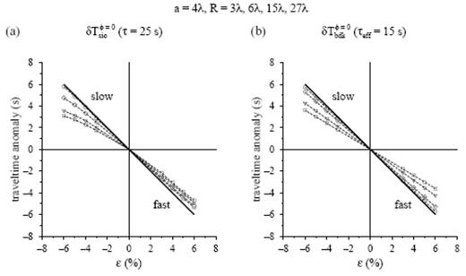
Same as Fig. 17, except that the quantities plotted in (a) are the traveltime shifts δTsioφ=0 measured by interactively aligning the initial upswings of the τ=25 s pulses phet(r, t) and phom(r, t), whereas the quantities in (b) are the shifts predicted by an effective banana–doughnut kernel Keff, with a reduced characteristic period τeff=15 s. Circles, diamonds, triangles and squares denote the measured and predicted traveltime shifts at distances R=3λ, 6λ, 15λ, and 27λ behind an S=10λ, a=4λ anomaly of varying magnitude, ε=±3, 4, 5, ±6 per cent. The unhealed Fermat anomaly δTferφ=0 is indicated by the ∼45° solid line in both plots.
app
App A: Ray Tracing Details
The rays and infinite-frequency wavefronts in Figs 8 and 10 were computed by solving an axially symmetric version of the first-order differential eqs (21) and initial conditions (22). We specify the instantaneous position of a point along a ray in terms of its cylindrical coordinates,
where q is the perpendicular distance from the axis and z is measured along it. The instantaneous direction of propagation of a wave along a ray can be written in the form
where i is the instantaneous angle between a ray and the z axis, considered to be positive if the ray is pointing towards the axis and negative if it is pointing away. The radius r in the specification (4) of the wave-speed anomaly is given in terms of the coordinates (A1) by
The absence of any dependence upon the cylindrical angle θ is what renders the problem axially symmetric. It is clear that a ray that leaves the source s in a given plane remains in that plane forever:
To find the remaining unknowns q, z and i needed to determine x and k^, we integrate the three equations
subject to the initial conditions
where dT is the differential traveltime along the ray and φ is the take-off angle at the source s, as illustrated in Fig. 3. Eqs (A5)–(A8) are equivalent to eqs (21) and (22). Wavefront snapshots are plotted by connecting adjacent points q(T, φ), z(T, φ) and q(T, φ+dφ), z(T, φ+dφ) at a fixed instant T.
The geometrical spreading factor (25) is given in this axially symmetrical situation by
where the partial derivatives ∂q/∂φ and ∂z/∂φ are computed at fixed traveltime T. As expected, the result (A9) reduces to ℒ=L in the case of a homogeneous medium, δc/c=0. There are two ways in which the spreading factor ℒ can vanish, indicating the presence of a caustic, either
or
The first condition, (A10), occurs whenever any ray other than φ=0 crosses the symmetry axis q=0; all of the rays in the same take-off cone φ≠0, 0≤θ≤2π, cross at the same point z, giving rise to the axial caustics seen in Figs 8 and 10. This caustic is associated with a closing of the ray tube in a direction ‘out’ of the invariable plane, (A4). The ‘funnel’ and ‘pencil point’ caustics in Figs 8 and 10 are, in contrast, due to closure (A11) of the ray tube within the plane. The axial caustic is said to be structurally unstable, because it would disappear in the absence of perfect axial symmetry. The cusped caustics are structurally stable, because distorted versions of them would persist.
References
Author notes
Now at: Department of Geosciences, National Taiwan University, Taipei, 106, Taiwan. E-mail: [email protected]
