The Fisher process of sexual selection with the coevolution of preference strength Free

Notation and modeling assumptions for the two frameworks we consider.

Definition	Population genetic models	Quantitative genetic models
Trait	Discrete: Locus T -T₁ allele, lacks trait -T₂ allele, expresses trait in males	Continuous: -Mean $\bar{z}$ -Variance $σ_{z}^{2}$
Preference	Discrete: Locus P -P₁ allele, lacks preference -P₂ allele, prefers T₂ males	Continuous: -Mean $\bar{y}$ -Variance $σ_{y}^{2}$
Preference strength (log scale in the quantitative genetic model)	Discrete: Locus A -A_i allele with preference strength α_i -Expressed only in females with P₂ allele	Continuous: -Mean $\bar{x}$ -Variance $σ_{x}^{2}$ -Larger $x$ means stronger preference
Genetic correlation or covariance	Genetic correlation emerges from model as a result of mating interactions: Two-locus: D_TP, D_TA, D_PA Three-locus: D_TPA	Genetic covariances between two traits derived assuming infinitesimal model: $B_{z y}$ ⁠, $B_{z y}$ ⁠, $B_{y x}$
Viability selection on trait	T₂ males are selected against with coefficient s	Stabilizing selection: $w_{m} (z) \propto e^{- \frac{z^{2}}{2 ω_{z}^{2}}}$ ⁠; Directional selection: $w_{m} (z) \propto e^{- λ z}$ ⁠. $ω_{z}^{2}$ and $λ$ are the strength of selection.
Mate choice	-Polygyny (all females have equal reproductive success) -P₁ females mate randomly -P₂ females (1 + α_i) times more likely to mate with a T₂ male than a T₁ male if encountering one of each	-Polygyny (all females have equal reproductive success) - Females mate according to Lande’s absolute preference function $ψ (z \| y, ν) \propto e^{- \frac{ν}{2} {(z - y)}^{2}}$
Preference mutation rate	Unidirectional mutation causing loss of preference (P₂ to P₁) at rate μ_P	N/A
Trait mutation rate	Unidirectional mutation causing loss of trait (T₂ to T₁) at rate μ_T	N/A

Definition	Population genetic models	Quantitative genetic models
Trait	Discrete: Locus T -T₁ allele, lacks trait -T₂ allele, expresses trait in males	Continuous: -Mean $\bar{z}$ -Variance $σ_{z}^{2}$
Preference	Discrete: Locus P -P₁ allele, lacks preference -P₂ allele, prefers T₂ males	Continuous: -Mean $\bar{y}$ -Variance $σ_{y}^{2}$
Preference strength (log scale in the quantitative genetic model)	Discrete: Locus A -A_i allele with preference strength α_i -Expressed only in females with P₂ allele	Continuous: -Mean $\bar{x}$ -Variance $σ_{x}^{2}$ -Larger $x$ means stronger preference
Genetic correlation or covariance	Genetic correlation emerges from model as a result of mating interactions: Two-locus: D_TP, D_TA, D_PA Three-locus: D_TPA	Genetic covariances between two traits derived assuming infinitesimal model: $B_{z y}$ ⁠, $B_{z y}$ ⁠, $B_{y x}$
Viability selection on trait	T₂ males are selected against with coefficient s	Stabilizing selection: $w_{m} (z) \propto e^{- \frac{z^{2}}{2 ω_{z}^{2}}}$ ⁠; Directional selection: $w_{m} (z) \propto e^{- λ z}$ ⁠. $ω_{z}^{2}$ and $λ$ are the strength of selection.
Mate choice	-Polygyny (all females have equal reproductive success) -P₁ females mate randomly -P₂ females (1 + α_i) times more likely to mate with a T₂ male than a T₁ male if encountering one of each	-Polygyny (all females have equal reproductive success) - Females mate according to Lande’s absolute preference function $ψ (z \| y, ν) \propto e^{- \frac{ν}{2} {(z - y)}^{2}}$
Preference mutation rate	Unidirectional mutation causing loss of preference (P₂ to P₁) at rate μ_P	N/A
Trait mutation rate	Unidirectional mutation causing loss of trait (T₂ to T₁) at rate μ_T	N/A

Table 1.

Notation and modeling assumptions for the two frameworks we consider.

Definition	Population genetic models	Quantitative genetic models
Trait	Discrete: Locus T -T₁ allele, lacks trait -T₂ allele, expresses trait in males	Continuous: -Mean $\bar{z}$ -Variance $σ_{z}^{2}$
Preference	Discrete: Locus P -P₁ allele, lacks preference -P₂ allele, prefers T₂ males	Continuous: -Mean $\bar{y}$ -Variance $σ_{y}^{2}$
Preference strength (log scale in the quantitative genetic model)	Discrete: Locus A -A_i allele with preference strength α_i -Expressed only in females with P₂ allele	Continuous: -Mean $\bar{x}$ -Variance $σ_{x}^{2}$ -Larger $x$ means stronger preference
Genetic correlation or covariance	Genetic correlation emerges from model as a result of mating interactions: Two-locus: D_TP, D_TA, D_PA Three-locus: D_TPA	Genetic covariances between two traits derived assuming infinitesimal model: $B_{z y}$ ⁠, $B_{z y}$ ⁠, $B_{y x}$
Viability selection on trait	T₂ males are selected against with coefficient s	Stabilizing selection: $w_{m} (z) \propto e^{- \frac{z^{2}}{2 ω_{z}^{2}}}$ ⁠; Directional selection: $w_{m} (z) \propto e^{- λ z}$ ⁠. $ω_{z}^{2}$ and $λ$ are the strength of selection.
Mate choice	-Polygyny (all females have equal reproductive success) -P₁ females mate randomly -P₂ females (1 + α_i) times more likely to mate with a T₂ male than a T₁ male if encountering one of each	-Polygyny (all females have equal reproductive success) - Females mate according to Lande’s absolute preference function $ψ (z \| y, ν) \propto e^{- \frac{ν}{2} {(z - y)}^{2}}$
Preference mutation rate	Unidirectional mutation causing loss of preference (P₂ to P₁) at rate μ_P	N/A
Trait mutation rate	Unidirectional mutation causing loss of trait (T₂ to T₁) at rate μ_T	N/A

Definition	Population genetic models	Quantitative genetic models
Trait	Discrete: Locus T -T₁ allele, lacks trait -T₂ allele, expresses trait in males	Continuous: -Mean $\bar{z}$ -Variance $σ_{z}^{2}$
Preference	Discrete: Locus P -P₁ allele, lacks preference -P₂ allele, prefers T₂ males	Continuous: -Mean $\bar{y}$ -Variance $σ_{y}^{2}$
Preference strength (log scale in the quantitative genetic model)	Discrete: Locus A -A_i allele with preference strength α_i -Expressed only in females with P₂ allele	Continuous: -Mean $\bar{x}$ -Variance $σ_{x}^{2}$ -Larger $x$ means stronger preference
Genetic correlation or covariance	Genetic correlation emerges from model as a result of mating interactions: Two-locus: D_TP, D_TA, D_PA Three-locus: D_TPA	Genetic covariances between two traits derived assuming infinitesimal model: $B_{z y}$ ⁠, $B_{z y}$ ⁠, $B_{y x}$
Viability selection on trait	T₂ males are selected against with coefficient s	Stabilizing selection: $w_{m} (z) \propto e^{- \frac{z^{2}}{2 ω_{z}^{2}}}$ ⁠; Directional selection: $w_{m} (z) \propto e^{- λ z}$ ⁠. $ω_{z}^{2}$ and $λ$ are the strength of selection.
Mate choice	-Polygyny (all females have equal reproductive success) -P₁ females mate randomly -P₂ females (1 + α_i) times more likely to mate with a T₂ male than a T₁ male if encountering one of each	-Polygyny (all females have equal reproductive success) - Females mate according to Lande’s absolute preference function $ψ (z \| y, ν) \propto e^{- \frac{ν}{2} {(z - y)}^{2}}$
Preference mutation rate	Unidirectional mutation causing loss of preference (P₂ to P₁) at rate μ_P	N/A
Trait mutation rate	Unidirectional mutation causing loss of trait (T₂ to T₁) at rate μ_T	N/A

Whether preferences evolve to be stronger or weaker can be important for several reasons. First, while preferences can result in sexual selection that leads to a wide array of unusual phenotypic traits in nature, comparative studies have shown that elaborate traits are often lost, possibly because preferences may be lost due to the evolution of weaker preference strength (reviewed in Wiens, 2001). If our basic models show the evolution of weaker preference strength, then this could provide a simple explanation for this loss of preference. Second, an understanding of whether preferences generally tend to evolve to be stronger or weaker in extensions of the Kirkpatrick (1982) and Lande (1981) models sets a baseline for the evolution of preference strength (e.g., a “null model,” according to Prum, 2010) that can be extended to more complex scenarios, such as speciation events, costs to choice, and good genes effects. Preference strength, often called “choosiness” in the speciation literature, has indeed been shown to evolve during speciation with gene flow, to be stronger under some conditions and weaker under others (Bürger & Schneider, 2006; Bürger et al., 2006; Cotto & Servedio, 2017; Kopp & Hermisson, 2008; Matessi et al., 2001; Otto et al., 2008; Pennings et al., 2008; Servedio & Bürger, 2015; Yukilevich & Aoki, 2022, reviewed in Kopp et al., 2018; Servedio & Boughman, 2017). Fully contextualizing these results, however, requires comparisons to the preference strength that would evolve in an isolated population (see e.g., Yeh et al., 2018).

We use population and quantitative genetic models to assess under what conditions stronger vs. weaker preferences will evolve in a single population, and how evolving preference strength affects the evolution of preferences and traits. We are interested in discovering the forces acting on preference strength that emerge from the action of sexual selection itself. Thus, we do not include costs to choice, which are well known to be a powerful force preventing or otherwise influencing the evolution of preferences in both population genetic (Bulmer, 1989; Pomiankowski, 1987) and quantitative genetic models (e.g., see Hall et al., 2000; Pomiankowski & Iwasa, 1998). Such costs would be expected to be stronger with higher preference strength (e.g., from risks incurred during a longer searching time, Byers et al., 2005, 2006; Hedrick & Dill, 1993, or a risk of going unmated, Gibson & Langen, 1996), so we would expect the evolution of higher preference strength to be more difficult with costs present than in the basal case we explore here.

We find that in the case of discrete traits studied by a population genetic model, preference strength evolves to be greater under the same conditions that cause preferences themselves to increase in frequency. However, selection for stronger preferences is very weak, even in comparison with indirect selection for the presence or absence of preferences in the Fisher process, and can often be overshadowed by genetic drift. Our quantitative genetic models show that a “runaway” to greatly exaggerated (or minimized) preference strength is unlikely when the male trait is under stabilizing viability and sexual selection. However, when the male trait is instead under directional viability selection, either a runway of increasing preference strength or evolution to random mating can occur if the initial preference strength is small or large enough, even when sexual selection is stabilizing as implemented by unimodal preferences. We conclude that the general shape of fitness functions (e.g., unimodal or monotonic) determined both by viability and by sexual selection are critical determinants of the evolution of preference strength.

Models of sexual selection

We use extensions of the classic population genetic and quantitative genetic models of Kirkpatrick (1982) and Lande (1981) to explore the cases of discrete and continuous preferences, respectively. However, there are many additional assumptions that must be made to apply these modeling techniques. Because of lack of enough data to allow generalizations about the genetics behind female preferences, we explore several different variants of these models (see Table 1).

For the case of discrete phenotypes, we use both two-locus and three-locus population genetic models, based on Kirkpatrick (1982). In the two-locus model we assume all females prefer one phenotype of a discrete male trait and assess coevolution of the trait locus with a locus controlling the strength of female preference. In the three-locus model we separate the female preference into two loci, one controlling whether females have a preference or not (if not, they are assumed to mate at random) and the second controlling the strength of the preference if it is present (see speciation models of the evolution of choosiness reviewed in Kopp et al., 2018; Servedio & Boughman, 2017). We also explore a variant of the three-locus model that includes genetic drift, to determine whether the effects that we see are strong enough to influence natural populations.

Our models of continuous preferences and traits, based on Lande (1981), generally assume a unimodal (absolute) preference function, which allows preference strength to be modeled as a separate parameter from the preference value itself (this is not possible with Lande’s (1981) psychophysical preference function, although this is also considered later to better understand the behavior of our main models). As discussed above, preference strength measures the width of this unimodal preference function. Following the assumptions of an infinitesimal model (Barton et al., 2017), genetic covariances among traits are modeled based on the phenotypic association among mated pairs, and the genetic variance is set as a parameter. We consider both cases of stabilizing selection and directional selection on the male trait.

Population genetic model

Model assumptions

We extend the classic haploid model of Kirkpatrick (1982) for the evolution of a sexual display trait with non-overlapping generations and a coevolving female preference to also include the evolution of preference strength. We assume a locus T (expressed only in males) codes for a costly display trait preferred by all females that mate non-randomly. Males with the T₁ allele do not express the trait and males with the T₂ allele do express the trait. A second locus P codes for the presence of a female preference. Females with the P₁ allele mate randomly, while females with the P₂ allele prefer T₂ males. The strength of this preference is given by the allele at the third locus, the A locus, where females with the A_i allele have preference strength α_i. Specifically, an A_i female with the P₂ allele is 1 + α_i times more likely to choose a T₂ male than a T₁ male if she were to encounter one of each. We thus have eight genotypes with the frequency of individuals carrying the genotype T₁P₁A₁, T₁P₁A₂, T₁P₂A₁, etc. denoted by f₁, f₂, f₃, and so on. Frequencies of alleles are denoted in lower case (e.g., t₂ is the frequency of the T₂ allele). In the absence of variation at the A locus (and without mutation, which we add below), the model reduces to that of Kirkpatrick (1982).

The first step in the life cycle is viability selection against displaying (T₂) males, with selection coefficient s. The genotype frequencies of females do not change following viability selection. The frequency of males with genotype j is denoted as f_j^` such that

\begin{array}{l} f_{j}^{'} = \frac{(1 - d_{j} s) f_{j}}{\sum_{k} (1 - d_{k} s) f_{k}}, \end{array}

(1)

with costs only experienced by displaying (T₂) males (d_j = 1 for j > 4 and 0 otherwise). Following viability selection each female chooses a mate. A polygynous mating system is assumed whereby all females have equal mating success (see also Kirkpatrick, 1982). This results in the frequency of mated pairs between a female with genotype i and a male with genotype j (M_ij) of

\begin{array}{l} M_{i j} = \frac{(1 + b_{i j} α_{c_{i}}) f_{i} f_{j}^{'}}{\sum_{k} (1 + b_{i k} α_{c_{i}}) f_{k}^{'}}, \end{array}

(2)

where c_i sets the parameter for the preferences strength coded for at the A locus, and is 1 for odd i and 2 for even i. b_ij accounts for the fact that T₂ males are preferred by non-randomly mating P₂ females with b_ij = 1 when j > 4 and i = 3, 4, 7, or 8 and b_ij = 0 otherwise. The denominator is the normalization to ensure each female has equal mating success. Next, recombination occurs between the loci at rate r, following the standard equations for three haploid loci. Finally, unidirectional mutation acts against the male trait and female preference such that a proportion µ_T of the T₂ alleles become T₁ alleles and a proportion of $μ_{P}$ of the P₂ alleles become P₁ alleles. The assumption of unidirectional mutation represents the case of a genetically complex trait that is more easily destroyed than created by mutation. Mutation plays the important role of maintaining variation in the trait and thus permitting linkage disequilibrium between the preference loci and the trait locus to persist indefinitely. Given that this role could also be played by bidirectional mutation, we do not expect our results to be highly sensitive to this assumption. All analyses of the population genetic models were carried out in Mathematica (Wolfram Research, Inc., 2020) and the code is archived on Dryad [see Data availability statement].

Two-locus model

We begin by analyzing a special case of the full model presented above with no variation in the P locus (p₂ = 1), such that all females mate preferentially with T₂ males according to the preference strength coded by their A locus (reducing the problem to a two-locus model). This model still collapses to Kirkpatrick (1982), with a fixed preference p₂ = 1, when $α_{1} = 0$ ⁠. Frame and Servedio (2012) presented such a model in the context of sensory bias (among several models in that paper) showing only that the change in frequency of a preference strength allele is very small between generations. We add unidirectional mutation to this model and analyze it more thoroughly here.

We begin by noting the evolutionary forces that act on preference strength. Recall that preference strength does not affect the viability or mating success of the females that express it: preference strength evolves only through indirect selection resulting from linkage disequilibrium that builds with the male trait. This linkage disequilibrium is positive as long as α₂ > α₁ (i.e., stronger preference strength becomes associated with the trait, determined analytically under weak selection and confirmed with numerical analysis for strong selection, see Supplementary File S1), suggesting that whenever the display trait can evolve to reach mutation-selection balance, ever-increasing values of the allele for higher preference strength evolves as well.

We must thus examine invasion of the male trait. We first fix preference strength by setting the frequency a₂ = 0, and then analyze the resulting one-dimensional model. We find two equilibria for the male trait: loss (t₂ = 0) and mutation-selection balance (⁠ $t_{2} = \frac{- α_{1} (1 - μ_{T}) + s (1 + α_{1}) (1 - μ_{T}) + 2 μ_{T}}{(s (1 + α_{1}) - α_{1}) (1 + μ_{T})}$ ⁠, approximately 1 when the mutation rate µ_T is small). Under these conditions of random mating, the male trait evolves (i.e., t₂ = 0 is unstable) whenever

\begin{array}{l} α_{1} > \frac{s (1 - μ_{T}) + 2 μ_{T}}{(1 - s) (1 - μ_{T})}, \end{array}

(3)

which is approximately given by α₁ > s/(1 − s) when the mutation rate µ_T is small. In summary, the male display trait can evolve so long as the preference strength is strong enough.

Because preference strength only evolves as a result of indirect selection through linkage disequilibrium with the male trait, preference strength can only be selected when variation in the male trait is maintained, otherwise preference strength becomes neutral. Since the male trait is lost whenever α₁ < s/ (1 − s), approximately, the evolution of preference strength cannot proceed under these conditions. In other words, given the above conditions for the strengths of viability selection and preference strength, when the trait is lost, there should be a line of infinitely many neutral equilibria for the final frequency of the preference strength allele.

If we restrict ourselves to the cases where the initial preference strength is sufficient for the male trait to evolve to mutation-selection balance, we find analytically (see Supplementary File S1) that there are two biologically feasible equilibria. Specifically, the frequency of the preference strength a₂ always evolves to fixation or loss; variation in preference strength is never maintained. To determine the direction of evolution of preference strength, we consider the invasion of an initially rare mutant preference strength, where the A₁ allele with preference strength α₁ is the resident (a₁ is approximately 1) and the A₂ allele with preference strength α₂ is the invader (a₂ is approximately 0). For simplicity, we will consider the evolution of preference strength as a series of such invasions. Assume that resident preference strength α₁ satisfies the conditions in inequality (3), such that the male trait can evolve and is maintained at mutation-selection balance. The invasion of A₂ will be successful when the resident-only equilibrium is unstable. Further, since we have shown that there are no polymorphic equilibria at the A locus provided the male trait is maintained, successful invasion implies the fixation of A₂.

We performed a linear stability analysis on the resident-only equilibrium. Numerical assessment of the eigenvalues, examined across a range of preference strengths α₁ and α₂ from 0 to 100 at s = 0.1, 0.4 and μ_T = 0.01, 0.001, indicate that a higher preference strength seems to always invade as long as the male trait evolves (Figure 1). This makes sense as preference strength evolves only through indirect selection and stronger preference strengths are expected to become associated with the male trait. This continuously drives up the frequency of an allele for stronger preference strength even though the male trait remains at mutation-selection balance. Thus, there is not an evolutionarily stable preference strength. Rather, preference strength evolves in a runaway fashion with increasingly strong preference strength invading ad infinitum whenever the male trait is maintained.

Figure 1.

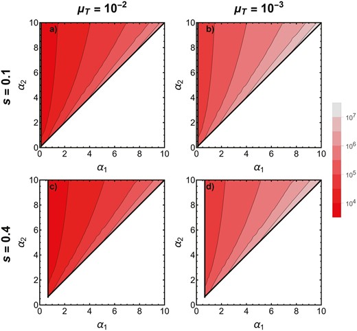
The direction and rate of evolution of preference strength in the two-locus model. The x-axis shows the resident preference strength and the y-axis shows the invading preference strength. Within the thick, black contours (colored in red), invasion of an allele for preference strength is successful. Clearly, only stronger preference strengths ever invade. As the color becomes brighter red, invasion occurs more quickly (see legend, which represents the number of generations to fixation). Note that the rate of fixation is presented on a log scale. We define fixation by stopping the recursion once a₂ > 0.999.

The evolution of preference strength is typically quite slow, as it relies on indirect selection and thus requires that variation be maintained in the male trait (here, through high mutation rates; Figure 1). More specifically, the rate of fixation for higher preference strength alleles varies dramatically based on both the mutation rate and the resident and invading preference strengths. When the resident preference strength is low (α₁ < 1), the invading preference strength α₂ is more than twice as strong, and the mutation rate is quite high (µ_T = 0.01; as may mimic a quantitative trait controlled by many loci), the allele for higher preference strength can effectively fix (measured as being above 0.999) in under ten-thousand generations. This, however, seems to be a lower bound on the time to fixation. Most cases require at least tens of thousands if not millions of generations before an allele for preference strength fixes. In general, fixation proceeds slower given stronger resident preference strength and smaller differences between the resident and the invader (Figure 1).

Three-locus model

We now return to the case with variation at the P locus. The results from this full, three-locus model closely follow those of the two-locus model. Specifically, we see that either the male trait is able to evolve and is followed by (weak) runaway selection for ever increasing preference strength, or the male trait does not evolve and preference strength becomes neutral.

Quasi-linkage equilibrium approximation

To better understand the behavior of the system, first we use a quasi-linkage equilibrium (QLE) approximation with an assumption of weak selection, including weak preference strength, to obtain approximate expressions for the linkage disequilibria (Supplementary File S1). We assume α₂ = α₁ + ε, where ε is a small, positive constant, so α₂ > α₁ and evolution is proceeding in small steps. We find that, to the first order in the weak parameters,

\begin{array}{l} {\hat{D}}_{T P} = \frac{1}{2} p_{2} (1 - p_{2}) t_{2} (1 - t_{2}) (α_{1} + ϵ α_{2}), \end{array}

(4a)

\begin{array}{l} {\hat{D}}_{A T} = \frac{1}{2} a_{2} (1 - a_{2}) t_{2} (1 - t_{2}) p_{2} ϵ, \end{array}

(4b)

\begin{array}{l} {\hat{D}}_{A P} = 0, \end{array}

(4c)

\begin{array}{l} {\hat{D}}_{A T P} = \frac{a_{2} (1 - a_{2}) p_{2} (1 - p_{2}) t_{2} (1 - t_{2}) r_{T P} (1 - r_{A P}) ϵ}{2 (r_{T P} (1 - r_{A P}) + r_{A P})} . \end{array}

(4d)

Perhaps the most important result is that the evolution of preference strength occurs primarily through linkage disequilibrium with the male trait (including via D_ATP which represents the three-way linkage disequilibrium). There is no evolutionary contribution (to the first order) to the spread of an allele at the A locus via linkage disequilibrium between the loci for the female preference and preference strength D_AP. Furthermore, we see that, to the first order, D_AT > 0 (as is D_ATP). This again shows that positive linkage equilibrium builds between the male trait and the locus for preference strength, such that selection favoring the trait leads to indirect selection for a stronger preference. Equation (4) thus suggests that whenever the male trait evolves, preference strength also evolves in a runaway fashion, with ever increasing preference strength able to invade.

The QLE analysis was repeated assuming strong resident preference strength α₁ (Supplementary File S1). Interestingly, this results in the QLE expression for linkage disequilibrium between the A locus and each other locus being 0 to the first order. This mirrors the result from the two-locus model, that selection becomes weaker (and thus invasion takes longer) with a stronger resident preference strength.

Numerical results

The above results rely on assumptions such as weak selection and mutations of small effect. To test their robustness, we also investigated the three-locus model with numerical approaches again focusing on a rare invading male trait and preference strength (with each allele at the P locus having an initial frequency of 0.5). We now assume only free recombination between loci. The general conclusions from the QLE approximation hold upon relaxing the assumption of weak selection. Specifically, increasing preference strength evolves whenever the male trait is maintained in the population at mutation-selection balance. We also find close agreement between the two-locus and three-locus population genetic models in other regards. In particular, extending results from the two-locus to the three-locus model suggests that T₂ is able to evolve if

\begin{array}{l} p_{2} α_{1} > \frac{s (1 - μ_{T}) + 2 μ_{T}}{(1 - s) (1 - μ_{T})} . \end{array}

(5)

This is identical to Equation (3) when we multiply preference strength by the frequency of females that express the preference p₂ (when p₂ = 1, we recover the result from the two-locus model). Note that associations between the P and A loci mean that inequality (5) is not exact, but since these associations have been shown to be weak (0 to the first order; Equation (4c)), this is likely a good approximation. Equation (5) is supported by numerical results.

More generally, we find that the three-locus model contains three regimes (Figure 2). In regime 1, inequality (5) is not satisfied and the male trait cannot evolve. In regime 2, inequality (5) is initially satisfied given the starting frequency of the preference, but mutation pressure against the male trait is weak. As a result, although the male trait can evolve to mutation-selection balance, very little variation in the male trait is maintained. This leads to weak linkage disequilibrium between the male trait and female preference, which in turn causes the loss of the female preference due to mutation pressure on the preference itself. Consequently, very few females prefer the costly display trait, and it is lost from the population. In regime 3, inequality (5) is satisfied and the mutation pressure against the male trait is strong. Due to high mutation rates, greater variation in the male trait and linkage disequilibrium between the trait and preference are maintained and the female preference remains in the population. In this regime, the evolution of preference strength proceeds in a runaway fashion such that a higher preference strength will always evolve. This gives the counterintuitive result that the male trait can only be maintained if there is strong mutation pressure against it. In Supplementary Appendix I, we show that when the P locus controls the direction of preference (i.e., P₁ females now prefer T₁ males) and the preferences P₁ and P₂ are roughly similar in strength, preference strength no longer evolves to fixation or loss; rather, little evolution occurs at the A locus which instead approaches a neutrally stable equilibrium.

Figure 2.

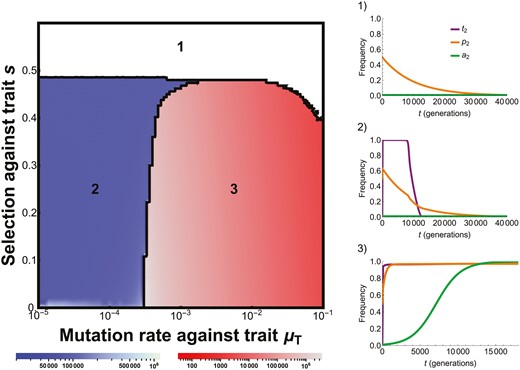
Numerical results from the three-locus model demonstrate the presence of 3 regimes (shown by color), the time until equilibrium is reached (shading; recursions stopped when each allele frequency changed by <10⁻⁸), and example timeseries from each regime. Regime 1 (white) occurs when there is insufficient female preference to drive the evolution of the male display trait. Regime 2 (blue) occurs when the male trait evolves, but not enough variation in it is maintained (due to low mutation pressure), leading to the ultimate loss of first the preference and then the trait. Regime 3 (red) occurs when the male trait evolves and enough variation in it is maintained (due to high mutation pressure) to prevent the loss of the preference and trait, and allow the evolution of preference strength (see main text). Initial conditions are p₂ = 0.5 (µ_P = 10⁻⁴), t₂ = 0.001, and a₂ = 0.001 (where α₁ = 2 and α₂ = 4). Timeseries parameters: (1) µ_T = 10⁻³, s = 0.6; (2) µ_T = 10⁻⁵, s = 0.2; (3) µ_T = 10⁻², s = 0.2.

Population genetic model with drift

One of the clearest takeaways from the population genetic models is that the evolution of preference strength relies on weak evolutionary forces. This begs the question of whether preference strength could evolve in a predictable fashion given stochasticity. To assess this, we created an individual-based model consistent with the three-locus population genetic model described above.

We assume a population has N/2 male and N/2 female individuals with the population size fixed at N for each non-overlapping generation. Each female reproduces once. If she carries the P₁ allele, she mates randomly. If she carries the P₂ and A_i allele, she chooses a mate by weighting all T₂ males by (1 + α_i) and selecting stochastically. Consequently, males mate anywhere from 0 to N/2 times per generation. Following reproduction, recombination occurs freely and two new haploid offspring (one male and one female) are created per mating (sampling all possible offspring with replacement). Offspring inheriting the T₂ (P₂) allele have it mutate to T₁ (P₁) with probability µ_T (µ_P). Mechanistically adding stochasticity at each step in an individual-based model, as opposed to adding stochasticity in an ad hoc manner to the deterministic model, allows for a more realistic assessment of the population size required for predictable evolutionary patterns to result.

With stochasticity, the fixation probability for higher preference strength is only appreciably different from the neutral case when there are relatively large populations and high mutation rates (Table 2). In particular, the mutation rates often must be unrealistically high (on the order of 0.1 in very small populations but still around 10⁻⁴ in larger populations) in order for preference strength to faithfully evolve to fixation.

Table 2.

Fixation probability (after 1000 runs) and mean time to fixation/loss of A₂ with α₂ = 4 and α₁ = 2 at various population sizes N and mutation rates µ_T, where s = 0.1 and µ_P = 10^-4 (thus, in the deterministic case, A₂ would always go to fixation). Likelihood is the probability of observing a fixation probability at least as different from 0.5 as observed (i.e., a two-sided test) assuming neutral evolution. Simulations were initiated with N/2 male and N/2 female individuals, with each having their genotype drawn randomly with equal probabilities of acquiring x₁ and x₂ alleles (for x = T, P, and A). Note that due to computational time constraints the parameters N = 5000 and µ = 10^-4 were run only 575 times. Italics indicate a less than 5% chance that sampling error alone led to deviations from a fixation probability of 0.5.

N	µ	Fixation probability	Mean time to fixation/loss	Likelihood
100	10⁻⁴	0.50	127	0.97
100	10⁻³	0.51	128	0.59
100	10⁻²	0.50	129	0.97
100	10⁻¹	0.61	116	<10⁻¹⁰
500	10⁻⁴	0.47	657	0.11
500	10⁻³	0.51	689	0.68
500	10⁻²	0.54	671	0.01
500	10⁻¹	0.93	413	<<10⁻¹⁰
1000	10⁻⁴	0.53	1343	0.08
1000	10⁻³	0.52	1298	0.27
1000	10⁻²	0.61	1297	<10⁻¹⁰
1000	10⁻¹	0.99	532	<<10⁻¹⁰
5000	10⁻⁴	0.53	6714	0.13
5000	10⁻³	0.54	6579	0.01
5000	10⁻²	0.91	4916	<<10⁻¹⁰
5000	10⁻¹	1.00	793	<<10⁻¹⁰

N	µ	Fixation probability	Mean time to fixation/loss	Likelihood
100	10⁻⁴	0.50	127	0.97
100	10⁻³	0.51	128	0.59
100	10⁻²	0.50	129	0.97
100	10⁻¹	0.61	116	<10⁻¹⁰
500	10⁻⁴	0.47	657	0.11
500	10⁻³	0.51	689	0.68
500	10⁻²	0.54	671	0.01
500	10⁻¹	0.93	413	<<10⁻¹⁰
1000	10⁻⁴	0.53	1343	0.08
1000	10⁻³	0.52	1298	0.27
1000	10⁻²	0.61	1297	<10⁻¹⁰
1000	10⁻¹	0.99	532	<<10⁻¹⁰
5000	10⁻⁴	0.53	6714	0.13
5000	10⁻³	0.54	6579	0.01
5000	10⁻²	0.91	4916	<<10⁻¹⁰
5000	10⁻¹	1.00	793	<<10⁻¹⁰

Table 2.

Fixation probability (after 1000 runs) and mean time to fixation/loss of A₂ with α₂ = 4 and α₁ = 2 at various population sizes N and mutation rates µ_T, where s = 0.1 and µ_P = 10^-4 (thus, in the deterministic case, A₂ would always go to fixation). Likelihood is the probability of observing a fixation probability at least as different from 0.5 as observed (i.e., a two-sided test) assuming neutral evolution. Simulations were initiated with N/2 male and N/2 female individuals, with each having their genotype drawn randomly with equal probabilities of acquiring x₁ and x₂ alleles (for x = T, P, and A). Note that due to computational time constraints the parameters N = 5000 and µ = 10^-4 were run only 575 times. Italics indicate a less than 5% chance that sampling error alone led to deviations from a fixation probability of 0.5.

N	µ	Fixation probability	Mean time to fixation/loss	Likelihood
100	10⁻⁴	0.50	127	0.97
100	10⁻³	0.51	128	0.59
100	10⁻²	0.50	129	0.97
100	10⁻¹	0.61	116	<10⁻¹⁰
500	10⁻⁴	0.47	657	0.11
500	10⁻³	0.51	689	0.68
500	10⁻²	0.54	671	0.01
500	10⁻¹	0.93	413	<<10⁻¹⁰
1000	10⁻⁴	0.53	1343	0.08
1000	10⁻³	0.52	1298	0.27
1000	10⁻²	0.61	1297	<10⁻¹⁰
1000	10⁻¹	0.99	532	<<10⁻¹⁰
5000	10⁻⁴	0.53	6714	0.13
5000	10⁻³	0.54	6579	0.01
5000	10⁻²	0.91	4916	<<10⁻¹⁰
5000	10⁻¹	1.00	793	<<10⁻¹⁰

N	µ	Fixation probability	Mean time to fixation/loss	Likelihood
100	10⁻⁴	0.50	127	0.97
100	10⁻³	0.51	128	0.59
100	10⁻²	0.50	129	0.97
100	10⁻¹	0.61	116	<10⁻¹⁰
500	10⁻⁴	0.47	657	0.11
500	10⁻³	0.51	689	0.68
500	10⁻²	0.54	671	0.01
500	10⁻¹	0.93	413	<<10⁻¹⁰
1000	10⁻⁴	0.53	1343	0.08
1000	10⁻³	0.52	1298	0.27
1000	10⁻²	0.61	1297	<10⁻¹⁰
1000	10⁻¹	0.99	532	<<10⁻¹⁰
5000	10⁻⁴	0.53	6714	0.13
5000	10⁻³	0.54	6579	0.01
5000	10⁻²	0.91	4916	<<10⁻¹⁰
5000	10⁻¹	1.00	793	<<10⁻¹⁰

The unpredictability of the evolution of preference strength can be attributed to stochastic forces preventing strong linkage disequilibrium from consistently arising. As an illustration of this, we find that the mean linkage disequilibrium between the A and T loci (with α₁ = 2 and α₂ = 4) is 0.003 in simulation runs where A₂ fixes and 0.001 in simulation runs where A₁ fixes (with N = 100, µ = 0.1, and s = 0.1). Thus, it seems that the generation of strong linkage disequilibrium is the factor limiting the predictable evolution of stronger preference strengths.

Quantitative genetic models

Our quantitative genetic models consider three sex-limited quantitative traits (see Table 1). A male phenotype $z$ and female preference $y$ are assumed to have normal distributions $p (z)$ and $q (y)$ ⁠, with mean and variance $\bar{z}, σ_{z}^{2}$ and $\bar{y}, σ_{y}^{2}$ ⁠, respectively. Female preference strength is denoted by $ν$ (⁠ $ν \geq 0$ ⁠) and we assume preference strength on a log scale, $x$ ⁠, has a normal distribution $η (x)$ ⁠, with mean $\bar{x}$ and variance $σ_{x}^{2}$ ⁠. Therefore, $ν = e^{x}$ and the average preference strength is $\bar{ν} = e^{\bar{x} + σ_{x}^{2} / 2}$ ⁠. Hereafter we refer to $x$ as the log-preference strength, and a larger $ν$ or $x$ means stronger preference strength. We adopt the absolute preference function $ψ (z | y, ν)$ in Lande (1981) as

\begin{array}{l} \begin{array}{l} ψ (z | y, ν) \propto e^{- \frac{ν}{2} {(z - y)}^{2}} . \end{array} \end{array}

(6)

The preference is thus unimodal with females preferring a specific male trait value that matches their preference. The genetic covariance matrix of the three phenotypes is

\begin{array}{l} \begin{array}{l} M = (\begin{array}{l} G_{z} & B_{z y} & B_{z x} \\ B_{z y} & G_{y} & B_{y x} \\ B_{z x} & B_{y x} & G_{x} \end{array}), \end{array} \end{array}

(7)

where the additive genetic variance of the male trait, female trait, and log-preference strength are denoted as $G_{z}$ ⁠, $G_{y}$ ⁠, and $G_{x}$ ⁠, respectively, and $B_{i j}$ (⁠ $i, j = z, y, x$ ⁠) is the genetic covariance between trait $i$ and $j$ due to pleiotropy and non-random associations of alleles at different loci. In Supplementary Appendix IV, we show that $B_{y x}$ is of a higher order than $B_{z x}$ and $B_{z y}$ and thus can be ignored (analogous to the result for the three-locus population genetic model in Equation (4)). This is because $B_{x y}$ is formed by the correlation between $x$ and $y$ within mated pairs (see equation (A4.1)). However, since males do not express trait $x$ or $y$ ⁠, the correlation between $x$ of the male and $y$ of the female should result from a combination of the correlation between the male trait $z$ and female preference $y$ due to non-random mating, and the genetic correlation between $z$ and $x$ within males.

We assume females have an identical number of progeny, so there is no direct selection on female preference or on preference strength. After one generation of selection, the changes in the average values of the three traits are

\begin{array}{l} \begin{array}{l} (Δ \bar{z}, Δ \bar{y}, Δ \bar{x}) = (\frac{1}{2} \frac{G_{z}}{σ_{z}^{2}} S_{z}, \frac{1}{2} \frac{B_{z y}}{σ_{z}^{2}} S_{z}, \frac{1}{2} \frac{B_{z x}}{σ_{z}^{2}} S_{z}) . \end{array} \end{array}

(8)

Here $S_{z}$ is the selection differential on male trait $z$ ⁠, and the coefficient ½ accounts for sex-limited expression of z in males.

Stabilizing selection on the male trait

Under stabilizing selection towards an optimal phenotype $z = 0$ ⁠, the relative fitness function $w_{m} (z)$ is modeled as

\begin{array}{l} \begin{array}{l} w_{m} (z) \propto e^{- \frac{z^{2}}{2 ω_{z}^{2}}}, \end{array} \end{array}

(9)

where $ω_{z}^{2}$ indicates the strength of viability selection. In Supplementary Appendix II, we show that given weak sexual and viability selection (⁠ $σ_{z}^{2} ≪ {\bar{v}}^{- 1}, ω_{z}^{2}$ ⁠), the equilibrium is a surface in the space of { $\bar{x}$ ⁠, $\bar{y}$ ⁠, $\bar{z}$ }, given by

\begin{array}{l} \begin{array}{l} \hat{z} (\bar{x}, \bar{y}) \approx \frac{\bar{y}}{1 + {(\bar{ν} ω_{z}^{2})}^{- 1}} . \end{array} \end{array}

(10)

Equation (10) indicates that the mean male trait value will be closer to the mean female preference when the average preference strength $\bar{ν}$ is stronger.

We define an equilibrium as neutrally stable if after any small perturbation, the population will evolve to a new equilibrium, and the distance between the new and the original equilibrium point is of smaller or the same magnitude to that of the perturbation. Otherwise, the equilibrium is defined as unstable, but an unstable equilibrium does not necessarily imply unbounded evolution away from the equilibrium surface, since the evolutionary trajectory can settle elsewhere on the equilibrium surface after traveling a long distance. In Supplementary Appendix III, we show that an equilibrium is neutrally stable if and only if $\overset{⇀}{c} \cdot \overset{⇀}{n} < 0$ ⁠, where $\overset{⇀}{c} = (B_{z x}, B_{z y}, G_{z})$ is the evolutionary direction, and $\overset{⇀}{n} = (\frac{\partial \hat{z}}{\partial \bar{x}}, \frac{\partial \hat{z}}{\partial \bar{y}}, - 1)$ is the vector perpendicular to the surface.

Therefore, the stability of equilibria depends on the genetic variances and covariances. Unlike the classical model which takes genetic covariances as parameters (Lande, 1981), we assume genetic covariances will evolve with the trait values. Supplementary Appendices IV and V show that the genetic covariances $B_{z y}$ and $B_{z x}$ at equilibrium are

\begin{array}{l} \begin{array}{l} {\hat{B}}_{z y} \approx \frac{1}{2} \bar{ν} G_{z} G_{y}, \end{array} \end{array}

(11a)

\begin{array}{l} \begin{array}{l} {\hat{B}}_{z x} \approx \frac{1}{2} \frac{\bar{ν} G_{z} G_{x} \bar{y}}{1 + \bar{ν} ω_{z}^{2}} . \end{array} \end{array}

(11b)

${\hat{B}}_{z y}$ is proportional to the average preference $\bar{ν}$ and is always positive, while ${\hat{B}}_{z x}$ is positive when the preferences are positive (⁠ $\bar{y} > 0)$ ⁠, and negative when $\bar{y} < 0$ ⁠.

Contrary to the results of the population genetic models, where the preference strength often becomes exaggerated when the initial preference is strong enough and drift is absent, preference strength generally does not become exaggerated under a quantitative genetic model with stabilizing selection. Instead, under reasonable parameter values, there is a surface of equilibria consisting of points which are neutrally stable (Figure 3A) as long as female preference $\bar{y}$ is not too small or too large (not shown). Interestingly, the range of $\bar{y}$ under which the equilibria are neutrally stable is larger when the mean log-preference strength is larger. For example, given $G_{z} = G_{y} = σ_{x} = 1, G_{x} = 0.9$ (recall that $\bar{ν} = e^{\bar{x} + σ_{x}^{2} / 2}$ ⁠), the equilibrium becomes unstable only when $| \bar{y} | > 41$ for $\bar{x} = - 5$ ⁠, and $| \bar{y} | > 71$ for $\bar{x} = - 2$ (not shown in Figure 3A). However, analytical results show that equilibria are more likely to be unstable when either the genetic variances (⁠ $G_{y}$ or $G_{x}$ ⁠) or the average preference strength $\bar{ν}$ is larger (see equation (A5.3)).

Figure 3.

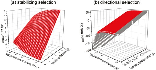
Equilibria and their stability under stabilizing and directional viability selection. For panel (A) $G_{z} = G_{y} = 1, σ_{x} = 1, h_{x}^{2} = 0.9$ ⁠, and for panel (B) $G_{y} = 3, σ_{x} = 1, h_{x}^{2} = 0.9, λ = 0.1$ ⁠. The red and gray color denote equilibria that are neutrally stable and unstable, respectively. Note that a larger $\bar{x}$ means stronger average preference $\bar{ν} = e^{\frac{σ_{x}^{2}}{2} + \bar{x}}$ ⁠.

It is important to note that our finding of stability of the surface in Figure 3A is dependent upon our assumption that genetic covariances will change as the preference, trait, and preference strength coevolve. Evolving genetic covariances are a realistic feature of coevolutionary processes. However, if we assume constant genetic covariances, as is more traditionally done in models of sexual selection, substantial portions of the surface in Figure 3A become unstable (see Supplementary Appendix VI).

For the special case when there is no variation, and thus no evolution, of preference strength, Lande (1981) shows that an equilibrium is neutrally stable when the genetic covariance between the male trait and female preference $B_{z y}$ is small enough relative to the genetic variance of the male trait $G_{z}$ ⁠, by taking the genetic covariance $B_{z y}$ as a parameter. When $B_{z y}$ can evolve, we show that the equilibrium instead will always be neutrally stable under weak selection (see Supplementary Appendix V, equation (A5.4)).

Directional selection on the male trait

The quantitative genetic model above predicts a much lower likelihood of runaway of preference strength than do our population genetic models. This could be because selection on the male trait is stabilizing, while the population genetic model instead assumes directional viability selection on the male trait, whereby one allele is always favored over the other. Therefore, we also analyze a quantitative genetic model assuming that the male trait is under directional selection, with the fitness function

\begin{array}{l} \begin{array}{l} w_{m} (z) = e^{- λ z}, \end{array} \end{array}

(12)

where $λ > 0$ measures the strength of viability selection.

Assuming weak sexual selection (i.e., $\bar{ν} σ_{z}^{2} ≪ 1$ ⁠), the equilibrium is (see Supplementary Appendix II).

\begin{array}{l} \begin{array}{l} \hat{z} (\bar{x}, \bar{y}) \approx \bar{y} - \frac{λ}{\bar{ν}} . \end{array} \end{array}

(13)

We find that the genetic covariance between the male trait and log-preference strength at equilibrium is ${\hat{B}}_{z x} \approx \frac{1}{2} G_{z} G_{x} λ$ ⁠, which does not change with the preference strength (see Supplementary Appendix V). Unlike the results under stabilizing selection where equilibria are neutrally stable at an intermediate range of mean preference $\bar{y}$ ⁠, under directional selection, the equilibria will be neutrally stable when the mean of the log-preference strength is within a certain range $x_{1} < \bar{x} < x_{2}$ ⁠, given that the genetic variance of the male trait $G_{x}$ ⁠, female preference $G_{y}$ ⁠, or the strength of viability selection $λ$ is small enough so that $λ \sqrt{G_{x} G_{y}} < 1$ (see Supplementary Appendix V). This is illustrated in Figures 3B and 4A (which show that this conclusion holds when the dynamics use freely evolving covariances). Analytical results also show that this range of $\bar{x}$ becomes wider when either of the genetic variances (⁠ $G_{y}$ or $G_{x}$ ⁠) or the strength of selection $λ$ is smaller (see equation (A5.6)).

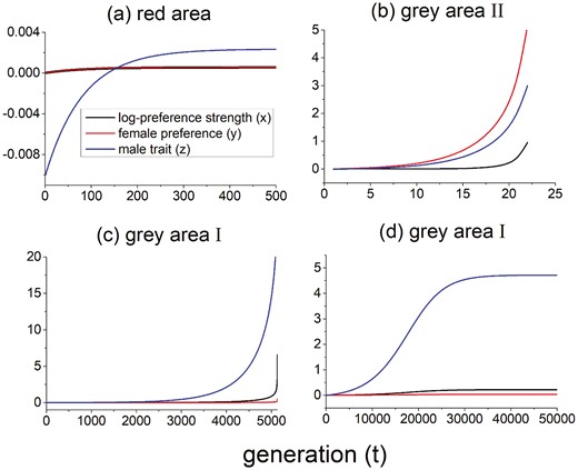
Temporal changes of the mean values of log-preference strength x¯, female preference y¯, and the male trait z¯ from their values at the original equilibrium after a downward perturbation from the surface in Figure 3B. For all panels, the population is initially at equilibrium and the perturbation decreases z¯ by 0.01. To calculate these trajectories, the genetic covariances are allowed to evolve based on equations (A4.11a) and (A4.11b) given in Supplementary Materials. Different panels show the dynamics from typical equilibria (x¯,y¯) in the three areas in Figure 3B. Panel (A) shows the point (−4,0) in the red area, and panel (B) shows the point (−0.5,0) in the gray area II. Panels (C) and (D) show equilibria in the gray area I, with the coordinates of (x¯,y¯) being (−7,0) and (−6,0) respectively. Note that the scale of the y-axis varies across panels, and in panel (A), the red and black lines overlap. Also, the recursion equations will be inaccurate when x¯ becomes large as they are derived under the assumption of weak sexual selection.

Figure 4.

Temporal changes of the mean values of log-preference strength $\bar{x},$ female preference $\bar{y}$ ⁠, and the male trait $\bar{z}$ from their values at the original equilibrium after a downward perturbation from the surface in Figure 3B. For all panels, the population is initially at equilibrium and the perturbation decreases $\bar{z}$ by 0.01. To calculate these trajectories, the genetic covariances are allowed to evolve based on equations (A4.11a) and (A4.11b) given in Supplementary Materials. Different panels show the dynamics from typical equilibria (⁠ $\bar{x}, \bar{y}$ ⁠) in the three areas in Figure 3B. Panel (A) shows the point (−4,0) in the red area, and panel (B) shows the point (−0.5,0) in the gray area II. Panels (C) and (D) show equilibria in the gray area I, with the coordinates of (⁠ $\bar{x}, \bar{y}$ ⁠) being (−7,0) and (−6,0) respectively. Note that the scale of the y-axis varies across panels, and in panel (A), the red and black lines overlap. Also, the recursion equations will be inaccurate when $\bar{x}$ becomes large as they are derived under the assumption of weak sexual selection.

When the initial preference strength is either too weak or strong, the equilibria become unstable, and runaway to either random mating or very strong preference and exaggerated traits can occur (gray areas in Figure 3B). The evolutionary dynamics show that in both gray areas I and II in Figure 3B, the system may runaway after a perturbation that moves the system downward off of the surface if it starts far from the stable area, as shown in Figure 4B and C. Specifically, after a downward perturbation, the population evolves towards to a higher male trait value $\bar{z}$ ⁠. However, both the log-preference strength $\bar{x}$ and preference $\bar{y}$ will also increase due to the genetic covariances $B_{z y}$ and $B_{z x}$ ⁠, and as a consequence, the new $\bar{z}$ is not high enough to arrive at the new equilibrium value $\hat{z} (\bar{x}, \bar{y})$ ⁠. The male trait, the preference and the preference strength will therefore continue to evolve upwards. An exception to these patterns occurs for equilibria in the gray area I that are close to the red area in Figure 3B. In this range, the system may evolve to a new stable equilibrium after a downward perturbation (the value of $\bar{z}$ “catches up” to the increasing value of $\hat{z}$ ⁠), but the distance between the new and the original equilibrium is much larger than the magnitude of the perturbation (see Figure 4D). Therefore, while these parts of the surface are unstable, perturbations off of them do not necessarily result in a runaway. On the other hand, if the perturbation moves the population upward from the equilibrium surface, the population will evolve to a lower preference strength, and finally to random mating (so that there will be no sexual selection). In this case viability selection will drive the male trait to be smaller and smaller. Thus, as in the population genetic model, strong initial preference strength can lead to the exaggeration of preference strength; however, in the quantitative genetic case, exaggeration of preference strength can also occur for very weak initial preference strength.

The reasons underlying the instability when the mean preference strength is small vs. large differ. Under a strong preference, the equilibria are unstable mainly because the genetic covariance between the male trait and female preference $B_{z y}$ becomes large, as found in Lande (1981). In contrast, under a weak preference, the equilibria are unstable mainly because as the mean preference strength changes, the equilibrium male trait value increases quickly (see Equation (13)). However, the genetic covariance $B_{z x}$ = $\frac{1}{2} λ G_{z} G_{x}$ does not change, so the male trait cannot evolve quickly to reach this equilibrium.

We should note, however, that when the mean preference strength evolves to be strong, the recursion equations, which assume weak sexual selection, will become inaccurate. Nevertheless, preference strength is not expected to evolve to be infinitely strong because the genetic covariance between the male trait and log-preference strength, $B_{z x}$ ⁠, will be small when the preference strength becomes too large; this is because in this case, females will almost always choose males with $\bar{z} = \bar{y}$ irrespective of their exact value of $x$ (see equation (A4.13) in Supplementary Appendix IV). Additionally, when the mean preference strength is very large, the genetic covariance between the male trait and female preference, $B_{z y}$ ⁠, will be large, indicated by Equation (11a). Since the evolutionary direction in the x-y-z space is $(B_{z x}, B_{z y}, G_{z})$ ⁠, the population will mainly evolve along the z-y plane under strong preferences (analogous to the slowing timescale of preference strength evolution when preference strength is strong in the population genetic models).

Discussion

Sexual selection can generate unusual phenotypes and play an important role in broader evolutionary phenomena such as speciation and extinction, but its power depends in part on the strength of mating preferences. Nevertheless, theoretical models of the evolution of preference strength, as opposed to preference direction or the value of the preferred phenotype, are rare in a general context. We establish “baseline models” of the evolution of preference strength, in the absence of direct costs to choice. Using extensions of classic population genetic and quantitative genetic models of sexual selection by Kirkpatrick (1982) and Lande (1981), we find the evolution of stronger or weaker preferences depends in part on which model was used, as summarized in Table 3. However, while the models differ fundamentally in what constitutes a preference or preference strength, and are thus difficult to compare, underlying patterns in the results hint at the importance of the form of viability and sexual selection (e.g., stabilizing or directional) on the male trait as the ultimate determinant of the evolution of preference strength.

Table 3.

Summary of key results of the two model frameworks.

Model version	Population genetic models	Quantitative genetic models
Stabilizing selection on the male trait	N/A	Equilibria are neutrally stable unless the trait that females prefer $\bar{y}$ ⁠, is extremely low or high.
Directional selection on the male trait	Two-locus model: Male trait is lost without sufficient preference strength; preference strength is then neutral Preference strength evolves in runaway fashion whenever the male trait can evolve Three-locus model: Male trait is lost without sufficient preference strength With high mutation rate and preference strength, male trait evolves and preference strength increases in runaway fashion With low mutation rate, male trait and preference strength initially increase but are ultimately lost	For some parameter values, there are stable equilibria when the average of log-preference strength $\bar{x}$ is within a range $[x_{1}, x_{2}]$ ⁠. Runaway may happen for equilibria with $\bar{x} < x_{1}$ or $\bar{x} > x_{2} .$ All equilibria will be unstable when the strength of viability selection, the genetic variance of the male trait, or female preference are too large.

Model version	Population genetic models	Quantitative genetic models
Stabilizing selection on the male trait	N/A	Equilibria are neutrally stable unless the trait that females prefer $\bar{y}$ ⁠, is extremely low or high.
Directional selection on the male trait	Two-locus model: Male trait is lost without sufficient preference strength; preference strength is then neutral Preference strength evolves in runaway fashion whenever the male trait can evolve Three-locus model: Male trait is lost without sufficient preference strength With high mutation rate and preference strength, male trait evolves and preference strength increases in runaway fashion With low mutation rate, male trait and preference strength initially increase but are ultimately lost	For some parameter values, there are stable equilibria when the average of log-preference strength $\bar{x}$ is within a range $[x_{1}, x_{2}]$ ⁠. Runaway may happen for equilibria with $\bar{x} < x_{1}$ or $\bar{x} > x_{2} .$ All equilibria will be unstable when the strength of viability selection, the genetic variance of the male trait, or female preference are too large.

Table 3.

Summary of key results of the two model frameworks.

Model version	Population genetic models	Quantitative genetic models
Stabilizing selection on the male trait	N/A	Equilibria are neutrally stable unless the trait that females prefer $\bar{y}$ ⁠, is extremely low or high.
Directional selection on the male trait	Two-locus model: Male trait is lost without sufficient preference strength; preference strength is then neutral Preference strength evolves in runaway fashion whenever the male trait can evolve Three-locus model: Male trait is lost without sufficient preference strength With high mutation rate and preference strength, male trait evolves and preference strength increases in runaway fashion With low mutation rate, male trait and preference strength initially increase but are ultimately lost	For some parameter values, there are stable equilibria when the average of log-preference strength $\bar{x}$ is within a range $[x_{1}, x_{2}]$ ⁠. Runaway may happen for equilibria with $\bar{x} < x_{1}$ or $\bar{x} > x_{2} .$ All equilibria will be unstable when the strength of viability selection, the genetic variance of the male trait, or female preference are too large.

Model version	Population genetic models	Quantitative genetic models
Stabilizing selection on the male trait	N/A	Equilibria are neutrally stable unless the trait that females prefer $\bar{y}$ ⁠, is extremely low or high.
Directional selection on the male trait	Two-locus model: Male trait is lost without sufficient preference strength; preference strength is then neutral Preference strength evolves in runaway fashion whenever the male trait can evolve Three-locus model: Male trait is lost without sufficient preference strength With high mutation rate and preference strength, male trait evolves and preference strength increases in runaway fashion With low mutation rate, male trait and preference strength initially increase but are ultimately lost	For some parameter values, there are stable equilibria when the average of log-preference strength $\bar{x}$ is within a range $[x_{1}, x_{2}]$ ⁠. Runaway may happen for equilibria with $\bar{x} < x_{1}$ or $\bar{x} > x_{2} .$ All equilibria will be unstable when the strength of viability selection, the genetic variance of the male trait, or female preference are too large.

In both types of models, the male trait is the only character that is under direct selection; both preference and preference strength evolve due to indirect selection, predominantly via positive genetic correlations with the male trait due to non-random mating. It is thus logical that attributes of selection on the trait should be of great importance in determining the evolution of preference strength. In our population genetic models, we find broad conditions for “runaway” evolution of greatly exaggerated preference strength. Both viability selection and sexual selection in this model are directional in that one trait allele or the other at a time is uniformly of higher fitness (since there is no line of polymorphic equilibrium with mutation on the trait). When the preferred trait continually increases in frequency because of a selective advantage (as is possible when mutation maintains variation), so does any allele for stronger preferences. When we consider the quantitative genetic model with directional viability selection on the male trait, we also see some conditions (with high or low initial preference strength) where a “runaway” can occur. The fact that runaways only occur under restricted conditions in the quantitative genetic model might be because female preferences are not directional, but rather stabilizing under the unimodal (“absolute”) preference function. Consistent with this conjecture, when we examine a quantitative genetic model with directional female preference using Lande’s (1981) psychophysical model, the equilibrium surface is always unstable and runaways in preference strength can always occur (see Supplementary Appendix VII), parallel to the results of the population genetic model. However, note that the quantitative genetic model with directional sexual selection is not directly analogous to the population genetic model, because Lande’s (1981) psychophysical model confounds the capacity for preference and preference strength.

Similarly, the evolution of preference strength will be restricted when the predominant form of selection is stabilizing. In the population genetic model, this can be seen in Supplementary Appendix I, which examines a version of the model in which P₁ is a preference for T₁ males, while P₂ is a preference for T₂ males. In this model, sexual selection will not uniformly favor one trait over the other when preferences are polymorphic; alleles for higher preference strength are thus not swept to fixation via indirect selection. Indeed, Servedio and Bürger (2014) concluded that this model behaved in an analogous way to the quantitative genetic model of Lande (1982) when his preferences acted through an absolute preference function, but not a psychophysical one, in two-island models of speciation. In our quantitative genetic models, given weak viability selection (either stabilizing or directional), when female preferences are stabilizing, the surface of equilibria is stable in a large area of the parameter space where the preference strength will not evolve without bounds. Again, the results of the two types of models are analogous. Thus, to summarize, a comparison of the models considered in Supplementary Appendices I and VII with those in the main text demonstrate that directional, rather than stabilizing, natural and sexual selection lead to a greater propensity for preference strength to evolve to be greatly exaggerated. Differences between the population and quantitative genetic models can thus be attributed to differences in the fitness functions, highlighting that care must be taken when attempting to compare between these approaches.

The result that biased mutation against a trait can ultimately favor the trait through the maintenance of genetic variation has been found in a model of the Fisher process without coevolving preference strength (Veller et al., 2020) and has also been seen in quantitative genetic models (Pomiankowski et al., 1991). Here we show that biased mutation can also promote the evolution of stronger preferences. However, in the three-locus model, we show that under some conditions the indirect selection favoring stronger preferences can be so weak that it cannot even overcome biased mutation against the preference allele. Likewise, drift can prevent the evolution of preference strength unless populations are large and mutation pressure on the male display trait is extremely (likely unrealistically) high. These findings are consistent with the conclusions of Frame and Servedio (2012), where they note an extremely slow rate of evolution at the locus controlling preference strength.

Following the assumptions of an infinitesimal model, our quantitative genetic models included evolving genetic covariances between the male trait and female preference/preference strength, $B_{z y}$ and $B_{z x} .$ These covariances are generated through correlations among mated pairs due to non-random mating. Assuming weak sexual selection, we show that $B_{z y}$ and $B_{z x}$ are proportional to the average preference strength. In contrast to our models, many previous quantitative genetic models of sexual selection treat genetic covariances as fixed parameters, so that the stability of the equilibria often depends on the parameter values. In fact, compared to results under evolving genetic covariances, results with fixed genetic covariances (as in some previous models) show much larger swaths of the surface of equilibria that are unstable and allow runaway evolution of preference strength to proceed. Broadly, our work thus demonstrates the importance of allowing genetic covariances in quantitative traits to freely evolve.

The fact that preference strength evolves solely through indirect selection in our models means that the results of the “baseline models” analyzed here are quite vulnerable to change if direct selection, which is generally stronger than indirect selection, were present on preference strength. We expect that in natural populations direct selection in the form of search costs may usually act against the evolution of stronger preferences. Because this selection is both relatively well understood and has the obvious effect of making preference strength less likely to evolve, it was not considered here. Direct selection against stronger preferences also interacts with direct benefits of being choosy (having stronger preferences), such as when increased fertility, territory, etc., jointly determine the “relative searching time,” which can predict the level of choosiness (Courtiol et al., 2016; Etienne et al., 2014). These effects, along with indirect benefits emerging from “good genes” scenarios, may also lead to the evolution of preference strength, even when the indirect effects we see in our baseline model do not (e.g., in the setting of acceptance thresholds, Priklopil et al., 2015). In cases where direct selection is expected to be extremely weak or absent, the indirect evolutionary forces explored in the current models may play a bigger role in determining preference strength evolution. The fact that some conditions in the quantitative genetic model promote the evolution of random mating could help to explain the finding that elaborate traits are often evolutionarily lost (Wiens, 2001), although it is likely that direct selection against choosiness also contributes to this pattern.

The critical role of the form of viability and sexual selection in determining the evolution of preference strength implies that the shape of fitness functions may also play an important role in speciation. The evolution of stronger preference strengths, or stronger choosiness, in isolated populations will strengthen the initial reproductive isolation expected to be present whenever preferences are assortative (as may occur at the onset of secondary contact between partly diverged populations). Thus, directional viability and sexual selection would seem to set the stage for speciation to occur more easily. On the other hand, if viability and sexual selection on display traits are often stabilizing, the forces in our models will not tend to favor very strong preferences in isolated populations. Stabilizing selection may then constitute a set of conditions that are somewhat less favorable for speciation, if all else were equal. Of course, if strong preferences are prevented from evolving due to direct selection against them in isolated populations, this direct selection may prevent the evolution of reproductive isolation as well (Yukilevich & Aoki, 2022).

The frequency with which directional vs. stabilizing selection on male traits occurs in natural populations remains unclear (Kingsolver & Diamond, 2011; Kingsolver et al., 2001). Our models of the evolution of preference strength illustrate the importance of this factor, however. The form of preference functions is already known to play an important role in determining the role of sexual selection in speciation, i.e., whether it promotes or inhibits divergence (Lande, 1982, reviewed in Servedio & Boughman, 2017). Our results highlight one more reason that the type of preference function is important to study in natural systems.

Data availability

The code for this project (in Mathematica) is archived on Dryad at doi:10.5061/dryad.c59zw3rcm

Author contributions

The project was conceived by M.R.S. B.A.L. developed the population genetic models, M.R.S. did the QLE analyses, and K.X. developed the quantitative genetic models. All authors contributed ideas to all of the analyses, contributed heavily to the initial draft, and revised the manuscript.

Conflict of interest: The authors declare no conflicts of interest.

Acknowledgments

We would like to thank two anonymous reviewers, Lutz Fromhage, Megan Bishop, Isaac Linn, and especially Thomas Aubier for very useful comments on an earlier draft of this paper.

Funding

This work was supported by National Science Foundation Grant DEB 1939290 to M.R.S. B.A.L. was also supported by a Royster Fellowship from the UNC Graduate School.

References

Bergstrom

,

C. T.

, &

Real

,

L. A.

(

2000

).

Towards a theory of mutual mate choice: Lessons from two-sided matching

.

Evolutionary Ecology Research

,

2

,

493

–

508

.

. https://doi.org/10.1086/499375

Bulmer

,

M. G.

(

1989

).

Structural instability of models of sexual selection

.

Theoretical Population Biology

,

35

,

195

–

206

.

Bürger

,

R.

, &

Schneider

,

K. A.

(

2006

).

Intraspecific competitive divergence and convergence under assortative mating

.

American Naturalist

,

167

(

2

),

190

–

205

Bürger

,

R.

,

Schneider

,

K. A.

, &

Willendsdorfer

,

M.

(

2006

).

The conditions for speciation through intraspecific competition

.

Evolution

,

60

,

2185

–

2206

.

Byers

,

J. A.

,

Byers

,

A. A.

, &

Dunn

,

S. J.

(

2006

).

A dry summer diminishes mate search effort by pronghorn females: evidence for a significant cost of mate search

.

Ethology

,

112

(

1

),

74

–

80

. https://doi.org/10.1111/j.1439-0310.2006.01127.x

. https://doi.org/10.1086/497401

Byers

,

J. A.

,

Wiseman

,

P. A.

,

Jones

,

L.

, &

Roffe

,

T. J.

(

2005

).

A large cost of female mate sampling in pronghorn

.

American Naturalist

,

166

(

6

),

661

–

668

Cotto

,

O.

, &

Servedio

,

M. R.

(

2017

).

The roles of sexual and viability selection in the evolution of incomplete reproductive isolation: From allopatry to sympatry

.

American Naturalist

,

190

(

5

),

680

–

693

. https://doi.org/10.1086/693855

Courtiol

,

A.

,

Etienne

,

L.

,

Feron

,

R.

,

Godelle

,

B.

, &

Rousset

,

F.

(

2016

).

The evolution of mutual mate choice under direct benefits

.

American Naturalist

,

188

(

5

),

521

–

538

. https://doi.org/10.1086/688658

Edward

,

D. A.

(

2015

).

The description of mate choice

.

Behavioral Ecology

,

26

,

301

–

310

.

. https://doi.org/10.1098/rspb.2014.0190

Etienne

,

L.

,

Rousset

,

F.

,

Godelle

,

B.

, &

Courtiol

,

A.

(

2014

).

How choosy should I be? The relative searching time predicts evolution of choosiness under direct sexual selection

.

Proceedings of the Royal Society of London. Series B

,

281

(

1785

),

20140190

. https://doi.org/10.1002/ece3.273

Frame

,

A. M.

, &

Servedio

,

M. R.

(

2012

).

The evolution of preference strength under sensory bias: A role for indirect selection

.

Ecology and Evolution

,

2

(

7

),

1572

–

1583

Gibson

,

R. M.

, &

Langen

,

T. A.

(

1996

).

How do animals choose their mates?

Trends in Ecology and Evolution

,

11

(

11

),

468

–

470

. https://doi.org/10.1016/0169-5347(96)10050-1

Hall

,

D. W.

,

Kirkpatrick

,

M.

, &

West

,

B.

(

2000

).

Runaway sexual selection when female preferences are directly selected

.

Evolution

,

54

(

6

),

1862

–

1869

. https://doi.org/10.1554/0014-3820(2000)054[1862:RSSWFP]2.0.CO;2

PubMed

. https://doi.org/10.1006/anbe.1993.1176

Hedrick

,

A. V.

, &

Dill

,

L. M.

(

1993

).

Mate choice by female crickets is influenced by predation risk

.

Animal Behaviour

,

46

(

1

),

193

–

196

. https://doi.org/10.1086/658341

Henshaw

,

J. M.

, &

Jones

,

A.

(

2020

).

Fisher’s lost model of runaway sexual selection

.

Evolution

,

74

,

487

–

494

.

Kingsolver

,

J. G.

, &

Diamond

,

S. E.

(

2011

).

Phenotypic selection in natural populations: What limits directional selection?

American Naturalist

,

177

(

3

),

346

–

357

Kingsolver

,

J. G.

,

Hoekstra

,

H. E.

,

Hoekstra

,

J. M.

,

Berrigan

,

D.

,

Vignieri

,

S. N.

,

Hill

,

C. E.

,

Hoang

,

A.

,

Gibert

,

P.

, &

Beerli

,

P.

(

2001

).

The strength of phenotypic selection in natural populations

.

American Naturalist

,

157

(

3

),

245

–

261

. https://doi.org/10.1086/319193

Kirkpatrick

,

M.

(

1982

).

Sexual selection and the evolution of female choice

.

Evolution

,

36

(

1

),

1

–

12

. https://doi.org/10.1111/j.1558-5646.1982.tb05003.x

Kokko

,

H.

, &

Johnstone

,

R. A.

(

2002

).

Why is mutual mate choice not the norm? Operational sex ratios, sex roles and the evolution of sexually dimorphic and monomorphic signaling

.

Philosophical Transactions of the Royal Society B

,

357

,

319

–

330

.

. https://doi.org/10.1111/j.1420-9101.2008.01547.x

Kopp

,

M.

, &

Hermisson

,

J.

(

2008

).

Competitive speciation and costs to choosiness

.

Journal of Evolutionary Biology

,

21

(

4

),

1005

–

1023

Kopp

,

M.

,

Servedio

,

M. R.

,

Mendelson

,

T. C.

,

Safran

,

R. J.

,

Rodriguez

,

R. L.

,

Scordato

,

E. C.

,

Symes

,

L. B.

,

Balakrishnan

,

C. N.

,

Hauber

,

M. E.

,

Zonana

,

D. M.

, &

van Doorn

,

S. G.

(

2018

).

Mechanisms of assortative mating in speciation: Connecting theory and empirical research

.

American Naturalist

,

191

,

1

–

20

.

Kuijper

,

B.

,

Pen

,

I.

, &

Weissing

,

F. J.

(

2012

).

A guide to sexual selection theory

.

Annual Review of Ecology, Evolution, and Systematics

,

43

(

1

),

287

–

311

. https://doi.org/10.1146/annurev-ecolsys-110411-160245

. https://doi.org/10.1111/j.1558-5646.1982.tb05034.x

Lande

,

R.

(

1981

).

Models of speciation by sexual selection on polygenic traits

.

PNAS

,

78

(

6

),

3721

–

3725

.

Lande

,

R.

(

1982

).

Rapid origin of sexual isolation and character divergence in a cline

.

Evolution

,

36

(

2

),

213

–

223

Matessi

,

C.

,

Gimelfarb

,

A.

, &

Gavrilets

,

S.

(

2001

).

Long-term buildup of reproductive isolation promoted by disruptive selection: How far does it go?

Selection

,

2

,

41

–

64

.

. https://doi.org/10.1038/hdy.1980.36

O’Donald

,

P.

(

1980

).

Genetic models of sexual and natural selection in monogamous organisms

.

Heredity

,

44

(

3

),

391

–

415

Otto

,

S. P.

,

Servedio

,

M. R.

, &

Nuismer

,

S.

(

2008

).

Frequency-dependent selection and the evolution of assortative mating

.

Genetics

,

179

,

2091

–

2112

.

Pen

,

I.

, &

Weissing

,

F. J.

(

2000

).

Sexual selection and the sex ratio: An ESS analysis

.

Selection

,

1

,

111

–

122

.

Pennings

,

P. S.

,

Kopp

,

M.

,

Meszena

,

G.

,

Dieckmann

,

U.

, &

Hermisson

,

J.

(

2008

).

An analytically tractable model for competitive speciation

.

American Naturalist

,

17

,

E44

–

E71

.

Pomiankowski

,

A.

(

1987

).

The costs of choice in sexual selection

.

Journal of Theoretical Biology

,

128

,

195

–

218

.

Pomiankowski

,

A.

(

1988

).

The evolution of female preferences for male genetic quality

.

Oxford Surveys in Evolutionary Biology

,

5

,

136

–

184

.

. https://doi.org/10.1111/j.1558-5646.1991.tb02645.x

Pomiankowski

,

A.

, &

Iwasa

,

Y.

(

1998

).

Runaway ornament diversity caused by Fisherian sexual selection

.

PNAS

,

95

,

5106

–

5111

.

Pomiankowski

,

A.

,

Iwasa

,

Y.

, &

Nee

,

S.

(

1991

).

The evolution of costly mate preferences. I. Fisher and biased mutation

.

Evolution

,

45

(

6

),

1422

–

1430

Priklopil

,

T.

,

Kisdi

,

E.

, &

Gyllenberg

,

M.

(

2015

).

Evolutionarily stable mating decisions for sequentially searching females and the stability of reproductive isolation by assortative mating

.

Evolution

,

69

(

4

),

1015

–

1026

. https://doi.org/10.1111/evo.12618

Prum

,

R. O.

(

2010

).

The Lande-Kirkpatrick mechanism is the null model of evolution by intersexual selection: Implications for meaning, meaning, honesty, and design in intersexual signals

.

Evolution

,

64

(

11

),

3085

–

3100

. https://doi.org/10.1111/j.1558-5646.2010.01054.x

Reinhold

,

K.

, &

Schielzeth

,

H.

(

2015

).

Choosiness, a neglected aspect of preference functions: A review of methods, challenges and statistical approaches

.

Journal of Comparative Physiology A

,

201

,

171

–

182

.

. https://doi.org/10.1111/ele.12142

Ritchie

,

M. G.

(

1996

).

The shape of female mating preferences

.

PNAS

,

93

,

14628

–

14631

.

Rodríguez

,

R. L.

,

Boughman

,

J. W.

,

Gray

,

D. A.

,

Hebets

,

E. A.

,

Höbel

,

G.

, &

Symes

,

L. B.

(

2013

).

Diversification under sexual selection: The relative roles of mate preference strength and the degree of divergence in mate preferences

.

Ecology Letters

,

16

(

88

),

964

–

974

PubMed

Rosenthal

,

G. G.

2017

.

Mate choice: The evolution of sexual decision making from microbes to humans

.

Princeton University Press

.

Google Preview

. https://doi.org/10.1146/annurev-ecolsys-110316-022905

Servedio

,

M. R.

, &

Boughman

,

J. W.

(

2017

).

The role of sexual selection in local adaptation and speciation

.

Annual Review of Ecology, Evolution, and Systematics

,

48

(

1

),

85

–

109

. https://doi.org/10.1111/evo.12762

Servedio

,

M. R.

, &

Bürger

,

R.

(

2014

).

The counterintuitive role of sexual selection in species maintenance and speciation

.

PNAS

,

111

,

8113

–

8118

.

Servedio

,

M. R.

, &

Bürger

,

R.

(

2015

).

The effects of sexual selection on trait divergence in a peripheral population with gene flow

.

Evolution

,

69

(

10

),

2648

–

2661

Servedio

,

M. R.

, &

Lande

,

R.

(

2006

).

Population genetic models of male and mutual mate choice

.

Evolution

,

60

(

4

),

674

–

685

.

PubMed

. https://doi.org/10.1111/evo.13944

Veller

,

C.

,

Muralidhar

,

P.

, &

Haig

,

D.

(

2020

).

On the logic of Fisherian sexual selection

.

Evolution

,

74

(

7

),

1234

–

1245

Wiens

,

J. J.

(

2001

).

Widespread loss of sexually selected traits: How the peacock lost its spots

.

Trends in Ecology and Evolution

,

16

(

9

),

517

–

523

. https://doi.org/10.1016/s0169-5347(01)02217-0

Wolfram Research, Inc.

(

2020)

.

Mathematica, version

12.1

.

Google Preview

. https://doi.org/10.2307/3677205

Yeh

,

D. J.

,

Boughman

,

J. W.

,

Sætre

,

G. -P.

, &

Servedio

,

M. R.

(

2018

).

The evolution of sexual imprinting through reinforcement

.

Evolution

,

72

,

1336

–

1349

.

Champaign, IL

.

Yukilevich

,

R.

, &

Aoiki

,

F.

(

2022

).

Evolution of choosiness dictates whether search costs of mate choice enhance speciation by sexual selection

.

Journal of Evolutionary Biology

,

35

,

1045

–

1059

.

Zahavi

,

A.

(

1995

).

Altruism as a handicap: The limitations of kin selection and reciprocity

.

Journal of Avian Biology

,

26

(

1

),

1

–

3