


Abstract
Electroanatomical maps using automated conduction velocity (CV) algorithms are now being calculated using two-dimensional (2D) mapping tools. We studied the accuracy of mapping surface 2D CV, compared to the three-dimensional (3D) vectors, and the influence of mapping resolution in non-scarred animal and human heart models.
Two models were used: a healthy porcine Langendorff model with transmural needle electrodes and a computer stimulation model of the ventricles built from an MRI-segmented, excised human heart. Local activation times (LATs) within the 3D volume of the mesh were used to calculate true 3D CVs (direction and velocity) for different pixel resolutions ranging between 500 μm and 4 mm (3D CVs). CV was also calculated for endocardial surface-only LATs (2D CV). In the experimental model, surface (2D) CV was faster on the epicardium (0.509 m/s) compared to the endocardium (0.262 m/s). In stimulation models, 2D CV significantly exceeded 3D CVs across all mapping resolutions and increased as resolution decreased. Three-dimensional and 2D left ventricle CV at 500 μm resolution increased from 429.2 ± 189.3 to 527.7 ± 253.8 mm/s (P < 0.01), respectively, with modest correlation (R = 0.64). Decreasing the resolution to 4 mm significantly increased 2D CV and weakened the correlation (R = 0.46). The majority of CV vectors were not parallel (<30°) to the mapping surface providing a potential mechanistic explanation for erroneous LAT-based CV over-estimation.
Ventricular CV is overestimated when using 2D LAT-based CV calculation of the mapping surface and significantly compounded by mapping resolution. Three-dimensional electric field-based approaches are needed in mapping true CV on mapping surfaces.
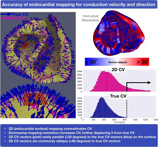
Leftward panel: Orientation vectors projecting from a basal view of the endocardium (blue, 3D true CV and pink, 2D CV). Top rightward panel: 3D and 2D CV vector parallel (<30° in blue) compared to oblique (>30° in red). Bottom rightward panel: Distribution histogram showing increased 2D CV (pink) compared to the 3D CV (blue). 2D, two-dimensional; 3D, three-dimensional; CV, conduction velocity; EAM, electroanatomical mapping; EGM, electrogram; LAT, local activation time; LV, left ventricle; RV, right ventricle; VT, ventricular tachycardia
Conduction velocity (CV) algorithms and directional vector maps have been integrated into electroanatomical mapping systems.
This study uses both animal experimental and human simulation data to highlight that ventricular CV measured on the two-dimensional (2D) surface overestimates the true three-dimensional CV.
2D CV vectors are rarely orientated parallel to the endocardial surface.
Reducing mapping resolution further reduces the accuracy of CV determination.
Introduction
Functional assessment of ventricular substrate to delineate the putative channels critical to ventricular tachycardia (VT) has been a paradigm shift in the ventricular electrophysiology field.1 This strategy aims to identify regions of slowed conduction or deceleration, which have been shown in both animal and human studies2 to correlate to critical isthmuses and are the desired target areas for catheter ablation. Fundamental to functional substrate characterization is an accurate calculation of conduction velocities (CVs). This is particularly relevant as automated CV algorithms and directional vector maps have been developed and integrated into electroanatomical mapping system modules. Various methods are used to calculate CV which most commonly involve interpolating the distances and differences between surface local activation times (LATs) and generating isochronal activation maps.3 However, these approaches have not been validated as they pertain to three-dimensional (3D) wavefronts and their activation on mapped two-dimensional (2D) surfaces.
The purpose of this study was to assess the accuracy of mapping surface-only 2D myocardial LATs to calculate CV and directional vectors, relative to using true 3D CV, in a Langendorff heart model which provoked further detailed experiments in a human computational model. In this model, we studied both sinus activation and right ventricular pacing. We examine (i) 2D CVs compared to true 3D CVs, (ii) differences in the angles of CV direction vectors between surface 2D CV and true 3D CV, and (iii) the effect of mapping resolution on such CV assessment.
Methods
Experimental model
Global transmural plunge needle mapping was performed in a healthy porcine explanted heart in a Langendorff perfusion setup as previously described.4 Twenty-five plunge needles (13 mm, 21 gauge) with four 36-gauge silver electrodes linearly spaced apart along each needle (100 total electrodes) were constructed by modifying a described method.5,6
Each electrode was 0.24 mm in diameter. The interelectrode spacing was 3 mm. To replicate a deep focal source, pacing was performed from a subendocardial electrode at a cycle length of 600 ms and twice diastolic threshold from the lateral LV wall by inserting these plunge needles in a 5 × 5 array with a spacing of 5 mm. In this arrangement, the innermost electrode was closest to the subendocardium, the outermost electrode was closest to the subepicardium, and the two inner electrodes were in the midmyocardium in relation to the subendocardium and subepicardium. Local activation time was recorded, and isochronal maps developed from the endocardium (pacing site), midmyocardium, and epicardium using Matlab software.
Computational model
Model geometry
A human ventricular model was used for our studies from an available segmentation of a MRI scan of an excised, normal heart.7 Fibre orientation was assigned from diffusion tensor images.
The segmentation was meshed with the software package Tarantula8,9 to yield 2.5 million nodes, comprising 3 million tetrahedra with an average element edge length of 0.5 mm. Additionally, four geometries of the same model were constructed, where we downsized the resolution of the initial geometry to 1 mm (290k nodes, 1.5 million tetrahedra), 2 mm (55k nodes, 300k tetrahedra), 3 mm (25k nodes, 120k tetrahedra), and 4 mm (7k nodes, 30k tetrahedra), respectively.
A previously developed Purkinje system10 was mapped into the geometry using universal ventricular coordinates.11 In brief, the Purkinje system was comprised of 1879 cable segments which were connected to the myocardium at 522 discrete Purkinje-myocyte junctions, with asymmetrical anterograde and retrograde conduction properties.
Electrophysiology model and simulations parameters
Two stimulation protocols were considered in our studies. These included His bundle pacing (sinus activation) and right ventricle (RV) apex pacing. For sinus activation, the proximal portion of the His cable was stimulated with a transmembrane current of 220 µA/cm2. For RV apex pacing, a transmembrane stimulus of 100 µA/cm2 was delivered to 1 mm3 volume centred at the RV apex on the endocardial side.
LATs were registered on the entire geometry for each protocol. Conduction velocities (direction and magnitude) were computed at every point in the whole mesh using the gradient of the LATs, which was termed 3D CV. In addition, we computed conduction velocities on the surface of the biventricular geometry using the gradient of surface-only LATs, which we termed 2D CV. This process was repeated for each mesh resolution. Thus, in total, we have 10 different simulations: two pacing protocols performed on the same geometry at five resolutions.
Monodomain simulations were performed using the Cardiac Arrhythmia Research Package.12 In the working myocardium, membrane kinetics were modelled with the 10 Tusscher-Panfilov human ventricular myocyte model. Conductivity values were chosen to produce conduction velocities of 70 cm/s along the fibre, 23.4 cm/s across the fibre in the sheet direction, and 23.4 cm/s in the transmural direction. In the Purkinje system, the same ionic model was used with parameters changed to better reflect Purkinje action potential duration. Conductivity in the Purkinje system was chosen to produce a CV of 2.5 m/s. A time step of 50 µs was used with a temporal output of 1 ms for all simulations. The total duration of each simulation was 650 ms.
Results
Experimental model
Transmural needle electrodes imbedded in healthy porcine ventricular tissue were used to calculate 3D and 2D CVs. Two-dimensional CV was determined for endocardial, mid-myocardial, and epicardial surfaces (Figure 1A). Three-dimensional CV was similar on both endocardial and epicardial sides, calculated to be 0.205 m/s on the endocardial surface and 0.254 m/s on the epicardial surface. Mean 2D CV on the epicardial surface was faster than the endocardial surface (0.509 m/s vs. 0.262 m/s) (Figure 1B). Furthermore, a rightward shift was observed when comparing the 3D CV to 2D CV, indicating higher overall 2D CV measurements (Figure 1C).
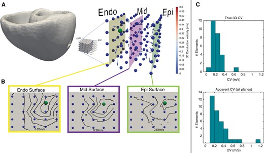
(A) Intramural needle electrodes demonstrating 3D CV (arrow vectors) from pacing source (ball). (B) 2D CV has been determined for each surface: endocardium, mid-myocardium, and epicardium. Note the approximately two-fold increase in CV on the epicardium. (C) Shows 3D and 2D CVs. CV, conduction velocity 2D, two-dimensional; 3D, three-dimensional.
Stimulation model
Sinus activation
Three-dimensional and 2D CV were assessed using five different, clinically applicable resolutions (average element edge-to-edge distance): 500 μm, 1, 2, 3 and 4 mm. Figure 2 show average CVs for 3D and 2D CV.
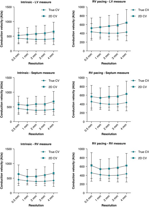
Average 3D and 2D CVs for each mapping resolution. CV, conduction velocity; 2D, two-dimensional; 3D, three-dimensional.
Two-dimensional CV was significantly faster than 3D CV across all mapping resolutions. Three-dimensional CV ranged between 200 and 800 mm/s. Average 3D endocardial LV CV were 429.2 ± 189.3, 410 ± 142.2, 393.4 ± 152.4, 391.4 ± 152.9, and 412.4 ± 199.3 mm/s for 0.5, 1, 2, 3, and 4 mm resolutions, respectively. Two-dimensional CVs were significantly faster at 527.7 ± 253.8, 554.6 ± 246.6, 584.8 ± 264.4, 602.9 ± 270.5, and 658.9 ± 321.5 mm/s for 0.5, 1, 2, 3, and 4 mm resolutions, respectively (all P < 0.01).
Three-dimensional endocardial septal CVs were 448.1 ± 199.6, 407.9 ± 139.3, 386.4 ± 140.8, 390.8 ± 151, and 421 ± 204.6 mm/s for 0.5, 1, 2, 3, and 4 mm resolutions, respectively. Two-dimensional CV was significantly faster at 581.5 ± 285.1, 555.5 ± 249.7, 593.8 ± 271.1, 593.7 ± 267.8, and 685.5 ± 344.7 mm/s for 0.5, 1, 2, 3, and 4 mm resolutions, respectively (all P < 0.01).
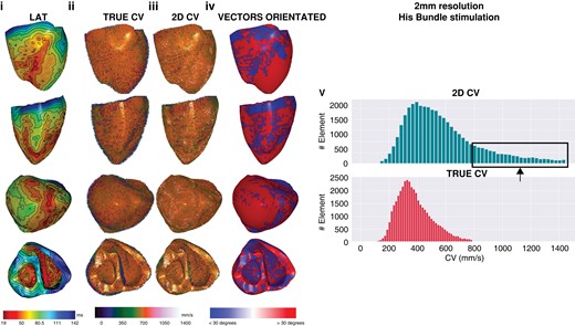
Lastly, endocardial RV 3D CVs were 468.6 ± 200.1, 411.5 ± 140.3, 392.5 ± 143.8, 381.4 ± 150, and 400.7 ± 184.2 mm/s for 0.5, 1, 2, 3, and 4 mm resolutions, respectively. Again, 2D CVs were all faster at 635.9 ± 316.5, 554.4 ± 243.2, 561 ± 244, 605.6 ± 281, and 670 ± 335.4 mm/s for 0.5, 1, 2, 3, and 4 mm resolutions, respectively (all P < 0.01). Examples of global LAT maps and distribution histograms of 3D vs. 2D CVs for 500 μm and 2 mm resolution are shown in Figures 3 and 4. Even at the highest resolution of 500 μm, there was rightward shifting of 2D CV, where CV exceeded 800 mm/s to a maximum of 1400 mm/s. As map resolution decreased, there was increasing rightward shift with a higher proportion of CV >800 mm/s.
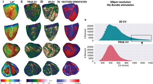
Five-hundred micrometre resolution, sinus activation. Global epicardial and endocardial LAT maps (i), CV vector maps for 3D (ii) and 2D CV (iii), CV vector surface orientation (iv), and CV histograms (v). CV, conduction velocity; LAT, Local activation time; 2D, two-dimensional; 3D, three-dimensional.
Two millimetre resolution, sinus activation. Note that as resolution progressively decreases, multiple small areas of early activation or ‘breakout’ are removed as resolution decreases, the percentage of faster CV when 2D CV increases and the proportion of CV vectors that are >30° increases. CV, conduction velocity; 2D, two-dimensional; 3D, three-dimensional.
Correlation coefficients were produced for 2D CV and 3D CV dividing the simulation model into 3 parts (RV, LV, and septum) to examine for regional differences in CV. As shown in Figure 5, for each pixel resolution, there were no differences in CVs between the different cardiac chambers. Overall, a trend showing decreasing correlation with decreasing resolution was demonstrated. The highest resolutions (500 μm and 1 mm) showed moderate correlation between 2D CV and 3D CV. As resolution decreased (2, 3, and 4 mm), correlation between 2D CV and 3D CV was weak.
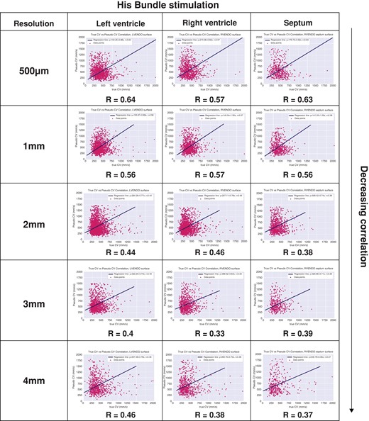
Correlation coefficients between mapped 3D CV and 2D CV. CV, conduction velocity; 2D, two-dimensional; 3D, three-dimensional.
RV pacing-generated wavefront
Similar to sinus activation, 3D CV for RV pacing ranged between 200 and 800 mm/s. Right ventricle pacing also demonstrated a rightward shift and progressive increase in 2D CV even at the highest resolution of 500 μm. Average 3D endocardial LV CVs were 433.6 ± 187.7, 413 ± 140.1, 400.7 ± 150.4, 401.9 ± 154.1, and 426.9 ± 197.4 mm/s for 0.5, 1, 2, 3, and 4 mm resolutions, respectively. Two-dimensional CVs were 516.7 ± 232.8, 540.6 ± 227, 564.7 ± 241.3, 587 ± 247, and 644.7 ± 296 mm/s for 0.5, 1, 2, 3, and 4 mm resolutions, respectively (all P < 0.01).
Three-dimensional CVs on the endocardial septum were 452.9 ± 190.8, 411.8 ± 135.8, 394.2 ± 139.1, 398.8 ± 150.6, and 434 ± 187.6 mm/s for 0.5, 1, 2, 3, and 4 mm resolutions, respectively. Two-dimensional CVs were significantly faster for all resolutions at 566.1 ± 257.6, 539 ± 225.4, 564.2 ± 236.2, 574.7 ± 238.8, and 627.1 ± 293 mm/s for 0.5, 1, 2, 3, and 4 mm resolutions, respectively (all P < 0.01).
Finally, 3D endocardial LV CVs were 464.1 ± 183.8, 414.7 ± 138.1, 396.2 ± 140.1, 395.9 ± 150.2, and 413.7 ± 182.3 mm/s for 0.5, 1, 2, 3, and 4 mm resolutions, respectively. All 2D CVs were faster at 620.8 ± 294.7, 539.2 ± 222.4, 549.1 ± 225.2, 573.6 ± 243.9, and 618.5 ± 276.7 mm/s for 0.5, 1, 2, 3, and 4 mm resolutions, respectively (all P < 0.01).
Correlation coefficients were generated for each site and resolution for RV pacing. There were no significant differences between LV, RV, and septal sites (Figure 6). However, as resolution declined, there was a trend showing decreasing correlation between 2D CV and 3D CV. Similar to sinus activation, there was moderate correlation at higher resolutions (500 μm and 1 mm) and weak correlation at lower pixel resolution (2, 3, and 4 mm).
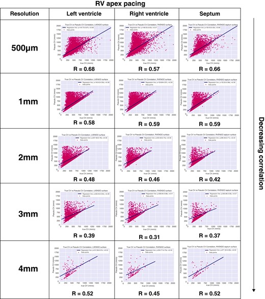
Correlation coefficients between mapped 3D CV and 2D CV. CV, conduction velocity; 2D, two-dimensional; 3D, three-dimensional.
Orientation of 3D CV vectors parallel to 2D CV vectors
The direction and angle of each CV orientation vector was applied to each mapping resolution in order to calculate the extent of CV that is parallel to the mapping surface. This was computed by comparing the angle between the two surface vectors (3D CV and 2D CV maps). The angle between 3D and 2D CV running parallel to the surface was defined as both vectors <30° (Graphical Abstract). Additional calculations were performed for <20° and <10°. These were generated for each mapping resolution and for both sinus activation and RV apical pacing.
As shown in Table 1, geometry resolution altered the interpretation of CV vector orientation. During sinus activation at a resolution of 500 μm, only 55.5% of CV vectors were <30° to the orientation of the 3D CV vectors. As resolution decreased, the proportion of CV vectors parallel to the surface progressively decreased to 31.3% at 4 mm resolution. There was no significant difference between sinus activation and RV apical stimulation for each resolution. The proportion of CV vectors <30° was 58.5% for 500 μm resolution which decreased to 35.9% at 4 mm resolution. As shown in Table 1, when the angle between 3D CV and 2D CV was reduced to <20° and <10°, the percentage of CVs vectors parallel to the surface reduced significantly as resolution of the geometrical mesh decreased.
Proportion of surface (apparent) CV vector parallel to endocardial mapping surface <30° (A), <20° (B), and <10° (C) and effect of decreasing mapping resolution and pacing wavefront
| Resolution | 0.5 MM | 1 mm | 2 mm | 3 mm | 4 mm |
|---|---|---|---|---|---|
| Angle <30° | |||||
| ȃSinus | 55.5% | 48.4% | 39.8% | 36% | 31.3% |
| ȃRV pacing | 58.5% | 51.7% | 43.9% | 40.5% | 35.9% |
| Angle <20° | |||||
| ȃSinus | 37.6% | 32.7% | 26.5% | 24% | 20.4% |
| ȃRV pacing | 40.1% | 35% | 29.2% | 26.9% | 23.9% |
| Angle <10° | |||||
| ȃSinus | 17.5% | 16.1% | 12.9% | 11.8% | 9.9% |
| ȃRV pacing | 18.8% | 17.4% | 14.4% | 13.4% | 11.3% |
CV, conduction velocity; RV right ventricle.
The orientation of 3D CV vectors oblique (>60°) the surface mesh was also analysed. As shown in Table 2, there was a progressive decrease in the proportion of 3D CV vector >60° to the angle of orientation of the surface mesh. Using sinus activation, at 0.5 and 4 mm resolutions, 57.6% and 31.4% of 3D CV vectors were >60° to the surface, respectively. The mismatch between 3D CV vectors and the surface was greater when RV apical stimulation was implemented. At 0.5 and 4 mm resolutions, 60.4% and 36.1% of 3D CV vectors were >60° to the surface. Less mismatch was seen when the angle was increased >70° and >80° but greater for RV apical pacing compared to sinus activation.
Proportion of surface (apparent) CV vector deviating from the endocardial mapping surface >60° (A), >70° (B), and >80° (C) and effect of decreasing mapping resolution and pacing wavefront
| Resolution | 0.5 MM | 1 mm | 2 mm | 3 mm | 4 mm |
|---|---|---|---|---|---|
| Angle >60° | |||||
| ȃSinus | 57.6% | 48.3% | 39.8% | 35.9% | 31.4% |
| ȃRV pacing | 60.4% | 51.7% | 43.5% | 40.5% | 36.1% |
| Angle >70° | |||||
| ȃSinus | 40.2% | 32.7% | 26.5% | 24.1% | 20.5% |
| ȃRV pacing | 42.7% | 35.1% | 29.2% | 27% | 24.1% |
| Angle >80° | |||||
| ȃSinus | 20.4% | 16.1% | 12.9% | 11.8% | 10% |
| ȃRV pacing | 21.9% | 17.4% | 14.3% | 13.5% | 11.4% |
CV, conduction velocity; RV right ventricle.
Discussion
The major findings of this study include the following:
Measurement of 2D surface LAT-based ventricular CV is a poor approximation of the 3D CV vectors as they are rarely orientated parallel to the endocardial surface.
2D CV overestimates true 3D CV causing a rightward shift of the CV histogram leading to measurement of supraphysiological 2D CVs, exceeding 800 mm/s.
This overestimation of 2D CV is similar in the endocardial RV, LV, and the interventricular septum and is not dependent on if the wavefront was sinus of RV pacing induced
Decreasing the simultaneous mapping electrode spacing resolution during 2D CV from 0.5 to 4 mm reduces the accuracy of the CV, displacing it further from the 3D CV.
Myocardial conduction velocity and reference standards
Integrating CV information is of great interest to the electrophysiology field as defining the functional elements of the substrate has been shown to correlate to critical VT circuitry components. This study highlights major discrepancies between surface-only mapping and true patterns of conduction in a healthy human simulation model, raising concerns as to the fundamental utility of ventricular CV mapping. As it pertains to this study in normal hearts, CV measurements when instrumentation is not limiting have been conducted in much detail.
Estimates of normal conduction have been defined in animal and human studies. In an isolated porcine heart, Kleber et al.13 demonstrated CVLongitudinal was 50.08 ± 2.13 cm/s and CVTransverse was 21 ± 0.94 cm/s. Others have demonstrated similar values in canine models ranging between CVLongitudinal of 50 and 60 cm/s and CVTransverse of 19 and 28 cm/s.14 In a normal human simulation model, we show CV histograms where mean CV ranges between 30 and 40 cm/s and rarely exceeded 80 cm/s. In models of ischaemia, CV has been shown to decrease abruptly to a CVLongitudinal of 31 ± 1 cm/s and CVTransverse of 13 ± 2 cm/s.13 Contemporary ventricular studies in swine and human infarct models corroborate slowed CV to be between 20 and 30 cm/s and very slowed conduction <10 cm/s.2
The tissue CV was intrinsically uniform over the ventricles. Differences in 3D CV are attributable to wavefronts approaching boundaries, wavefront collisions, negative wavefront curvature, and Purkinje involvement, which accelerate the CV, while positive wavefront curvature as emanating from a focal source will decrease the CV. Even in RV apex pacing, significant CV variation was noted, showing the effect of activity retrogradely entering the Purkinje and later exiting to decrease the activation time and suggesting higher CVs.
Methods and mathematical algorithms used to calculate CV
High-density mapping using regular-spaced, multi-electrode catheters record both electrograms and their spatial locations using an electroanatomical mapping system. These fixed-spacing platforms allow for assessment of CV. CV data are used clinically to delineate activation times either in sinus (or paced) rhythm or during arrhythmias. Until recently, current EAM systems were unable to support real-time, automated CV maps as offline analysis was required. New technology allows integrative activation maps or vector maps, which apply physiologically-based assumptions involving velocity continuity, minimizing errors in EAM timing, data projection and interpretation of complex EGMs. High-resolution maps are important to ensure accurate estimation of CV maps to satisfy the spatial Nysquist criterion that the interelectrode distance must be less than half the smallest relevant spatial wavelength.
The speed and direction of propagation of the AP wavefront defines CV. The maximum rate of change in cellular transmemebrane voltage defines activation time, correlating with the maximum negative derivative of the extracellular unipolar potential (-dV/dt) of the unipolar electrogram (EGM). Bipolar EGM surrogates also used include maximum and minimum absolute voltage and maximum absolute slope dV/dt. Annotated LATs are converted to isochronal lines and used as a visual representation of CV: widely spaced isochrones infer faster CV whereas regions of isochronal crowding are a surrogate of slow CV. However, unipolar EGMs are affected by far-field effects and bipolar EGMs change depending on the electrode position relative the propagation wavefront. Furthermore, the use of LAT-guided annotation alone can be misleading due to errors created by interpolation of projected points on a reconstructed chamber.2 This has led to alternative techniques used to analyse CVs including phase mapping and frequency domain analysis.15
Multiple mathematical approaches have been developed for CV estimation including the ‘average vector’ method where CV between a single point to five adjacent points along the activation front are averaged through regions of least isochronal crowding. CV between two points is calculated using the linear distance and difference in the LATs between these points. A more advanced method is the triangulation method which uses the spatial LAT coordinates from unipolar electrodes derived from the electroanatomical map to calculate CV using a trigonometric algorithm.16 As an example, the commonly used triangulation ‘single vector’ method assumes the tissue is homogenously anisotropic and 2D. This may overestimate CV by simplifying 3D pathways, assuming conduction takes the shortest course and neglects participation of depth propagation.2 Other methods include the finite difference, polynomial surface, vector loops, isopotential lines, arbitrary scalar fields and analytic expressions.16
A major potential limitation of these techniques is the use of 2D data (assuming conduction occurs along a single layer and orientation) which is inherently limited to calculate true wavefront speed. This is highly relevant in ventricular myocardium where transmural orientation of myofibres can be highly rotated.17 Three-dimensional reconstructed ex-vivo diffusion-weighted high-resolution imaging of the ventricular fibre microstructure has demonstrated fibre orientation in the transverse plane can rotate ±20–30°.17 Based on this, we selected a cut-off of <30° as an acceptable angle between 3D and 2D CV orientation vectors. Firstly, we show that a large proportion of 3D CV vectors do not run parallel with the surface. Secondly, we show that with greater mapping detail or resolution, more 2D CV vectors that run parallel to the surface will be added improving CV accuracy; however, even at the highest resolution of 500 μm, there was >40% mismatch between 3D and 2D CV vectors. We have also shown that wavefronts that are not travelling exactly tangential to the mapping surface will be overestimated. There was both an increasing rightward shift of 2D CV and weakening correlation coefficients as mapping resolution decreased. Regions of slowed CV in the unscarred cardiac model used in the current study were falsely increased with 2D surface-mapping only, plateauing when the mapping resolution >2 mm spacing. This is particularly important for thicker structures, such as ventricular myocardium, where transmural or 3D propagation is observed.16
As such, contemporary methods are imperfect and highly dependent on catheter orientation and position of the electrodes on the sampled tissue. Local activation time may be under sampled and inaccurate timings or false coordinate locations reduce the accuracy of CV calculation. Furthermore, these methods assume that conduction is planar along a 2D endocardial mapping surface omitting intramural contributions to a travelling wavefront. This is highly relevant as measuring transmural conduction that occurs deep in thick ventricular myocardium produces supra-physiological surface 2D CVs, as only the tangential component of the diverging wavefront on the surface is measured. This may also produce multiple simultaneous surface breakout sites that will complicate CV calculation.18
Contemporary automated CV algorithms in electroanatomical mapping systems
The Coherent Mapping Module (Biosense Webster Inc, Diamond Bar, CA, USA) is an automated proprietary algorithm included with the CARTO electroanatomical mapping system where the surface mesh is segmented into 3 mm triangles, each of which are assigned a LAT, conduction vector and probability of being of a slow or nonconductive (SNO) area. CV is calculated as part of the wave estimation, optimizing the measurements into a continuous wave propagation. One of the criteria for SNO zone indication is inconsistency in conduction (such as block or different conduction directions). SNO zones are also indicated for regions of very slow CV (<10 cm/s). Traces alone the wave propagation are used to visualize conduction, with heading wider than tail to represent direction. Additionally, fast CV is presented as thin and long arrow and slow CV represented as thick and short arrrow. The threshold for slow visualization is selected from a relative CV scale between 0 and 100 (where <20 defines the default for slow). The utility of CV vectors has previously only been assessed in the scarred atria2,19 applying physiological CV properties from normal healthy atria. Currently, the experience of validation of automated CV algorithms in 3D ventricular CV mapping is lacking.
Omnipolar mapping is an orientation and LAT-independent approach that is able to measure cardiac wavefront properties from a single location deriving beat-to-beat activation direction and CV from an electric field (E-field) using three triangular electrodes referred to as a clique where virtual EGMs or ‘omnipolar bipolar EGMs’ are generated. Calculation of direction activation and CV has been previously described and validated on planar wavefronts.20 Implementation of LAT-independent omnipolar mapping without the need for global mapping to calculate real-time directional and CV data has yet been studied in healthy or disease ventricular substrate and validated using 3D approaches, especially with omnipolar mapping.
Clinical significance
The implementation of surface isochronal and CV mapping to guide critical VT isthmus localization as a substrate-based ventricular mapping technique is increasingly used.21 Isochronal late activation mapping (ILAM) annotates the LAT to the latest activation and identifies regions of LAT isochronal crowding, also referred as ‘deceleration zones’.1,22 It essentially is a surface LAT measurement of CV. Based on the findings of the current study, 2D CV on the ventricular endocardial surface can greatly overestimate true 3D CV. Given these findings, it would be expected that deep sources, such as intramural or epicardial substrate, would erroneously affect surface CV estimation to a greater extent (see Supplementary material online, Figure S1). Ideker et al.23 has previously elegantly described the assumptions of isochronal mapping including the findings of the current study: the duration of surface activation is shorter as the depth from the source increases.24 This may be corrected if the angle of incidence (direction of the wavefront) is known. Furthermore, map point density can significantly impact surface CV determination. As shown in Table 1, CV accuracy deteriorates when map pixel density or resolution is >2 mm.
It may also be possible to manipulate the finding of erroneous CV heterogeneity and supraphysiological speed as a method to identify deep sources.25 Improvements in surface CV determination, closer to true 3D activation, will have major implications on using surface-based surrogates to uncover critical VT isthmus sites such as ILAM and other functional-based CV techniques.
Limitations
These findings are only applicable to normal ventricular myocardium as scarred substrate was not implemented in simulation models in the current study. Future studies incorporating models of transmural and non-ischaemic fibrosis assessing 2D CV and the impact on estimating regions of slow conduction are needed.
Conclusion
Myocardial surface 2D CV mapping overestimates true 3D CV, as the predominant direction of conduction vectors is rarely parallel to the surface, leading often to supra-physiological CV. Decreasing the resolution in simultaneous mapping array from 0.5 to 4 mm reduces the accuracy of estimating 3D CV using 2D LAT approaches. These finding suggest that 3D electric field-based algorithms and mapping tools will be needed for automated CV algorithms in ventricular electroanatomic mapping.
Supplementary material
Supplementary material is available at Europace online.
Funding
This work was supported by the Lefoulon Delalande Foundation.
Data Availability
Data is available on request from the authors.
References
Author notes
The first two share first authorship.
The last two authors share senior authorship.
Conflict of interest: R.A. is a recipient of the Royal Australasian College of Physicians (RACP) Bushell Travelling Fellowship. K.N. is a recipient of the Mid-career Investigator Award from the Heart & Stroke Foundation of Ontario. K.N. is research consultants for Biosense Webster, Blue Rock, Abbott & sevier. All remaining authors have declared no conflicts of interest.
