


Abstract
The Saltmarsh Sparrow (Ammospiza caudacuta) is a tidal marsh bird facing rapid population decline throughout its range, largely caused by degradation and loss of breeding habitat. Thus, there is a need to preserve tidal marshes in the northeastern United States, but to do so requires an understanding of the habitat features that support robust populations. Previous studies have shown Saltmarsh Sparrow abundance increases with marsh size, but in similar bird species, area sensitivity is more directly linked to edge avoidance. Whether additional landscape features affect the abundance of Saltmarsh Sparrows is unknown. We explored how the height of objects on the horizon, an index of habitat openness, affected the abundance of Saltmarsh Sparrows. Our primary goal was to determine whether the angle to the highest point on the horizon (“angle to maximum horizon”) predicted abundance better than marsh area or distance to the marsh edge. We used N-mixture models to evaluate the combination of spatial factors that best predicted Saltmarsh Sparrow abundance while also accounting for survey-level variables that could influence detection probability. We found that the interaction between distance to edge and angle to maximum horizon best predicted abundance. Taller objects on the horizon were negatively correlated with bird abundance, and this effect was strongest within 50 m of the marsh edge. When we considered the predictive powers of patch area, distance to edge, and angle to maximum horizon individually, angle to maximum horizon was the best single predictor. We found the highest abundance of Saltmarsh Sparrows at point locations where the angle to maximum horizon was 0.0°, and at angles greater than 12° the predicted abundance fell below 1 bird per survey point. We propose that managers should prioritize marsh openness and experimentally test the effect of marsh edge manipulations when making conservation decisions for this rapidly declining species.
Resumen
Ammospiza caudacuta es un ave de marisma que enfrenta una rápida disminución poblacional a través de su rango, causada en gran medida por degradación y pérdida de hábitat reproductivo. Por ende, hay una necesidad de preservar las marismas en el noreste de Estados Unidos, pero hacerlo requiere un entendimiento de las características del hábitat que mantienen poblaciones robustas. Los estudios previos han mostrado que la abundancia de A. caudacuta aumenta con la superficie de marisma, pero en especies similares de aves, la sensibilidad a la superficie está más directamente vinculada con la evasión del borde. Sin embargo, no se sabe si otras características del paisaje afectan la abundancia de A. caudacuta. Analizamos cómo el peso de los objetos en el horizonte, un índice de apertura de hábitat, afectó la abundancia de A. caudacuta. Nuestro objetivo principal fue determinar si el ángulo al punto más alto en el horizonte (“ángulo al máximo horizonte”) predecía mejor la abundancia que la superficie de marisma o la distancia al borde de la marisma. Usamos modelos de mezcla N para evaluar la combinación de factores espaciales que mejor predijeron la abundancia de A. caudacuta, contabilizando al mismo tiempo variables a nivel de muestreo que podrían influenciar la probabilidad de detección. Encontramos que la interacción entre distancia al borde y ángulo al máximo horizonte predijo mejor la abundancia. Los objetos más altos en el horizonte estuvieron negativamente correlacionados con la abundancia de aves, y este efecto fue más fuerte dentro de los 50 m del borde de la marisma. Cuando consideramos de modo individual el poder predictivo de la superficie de parche, la distancia al borde y el ángulo al máximo horizonte, el ángulo al máximo horizonte fue el mejor predictor individual. Encontramos la mayor abundancia de A. caudacuta en ubicaciones puntuales dónde el ángulo al máximo horizonte fue 0.0°, y en ángulos mayores a 12° la abundancia predicha cayó por debajo de un ave por punto de muestreo. Proponemos que los gestores deberían priorizar la apertura de las marismas y evaluar experimentalmente el efecto de la manipulación del borde de la marisma al tomar decisiones de conservación para esta especie que está disminuyendo rápidamente.
INTRODUCTION
Tidal marshes of North America support more endemic vertebrates than any other coastal marsh system in the world (Greenberg et al. 2006). These marshes are heavily impacted by coastal development (Batzer and Baldwin 2012) and sea levels that are rising faster than the global average (Kopp 2013, Yin and Goddard 2013). Many populations of tidal marsh birds are declining rapidly, likely because of this substantial habitat loss (Wiest et al. 2016, Correll et al. 2017). There is a clear need to preserve tidal marshes in the United States, but to do so requires an understanding of the habitat features that support robust populations of their endemic species.
The Saltmarsh Sparrow (Ammospiza caudacuta) is a tidal marsh bird exhibiting precipitous decline throughout its range (Correll et al. 2017). As a ground-nesting species, the Saltmarsh Sparrow is impacted by flooding from tides and storms (Shriver et al. 2007, Gjerdrum et al. 2008). Recent estimates suggest that nearly 80% of Saltmarsh Sparrow nests fail due to flooding (Ruskin et al. 2017), with this number expected to rise under even small increases in sea level (Bayard and Elphick 2011). Consequently, Saltmarsh Sparrows exhibit the highest documented rate of annual population decline (–9.0%) of any tidal marsh or passerine bird species in North America, and complete extinction is predicted within the next 50 yr without management intervention (Field et al. 2017, 2018, Correll et al. 2017, Roberts et al. 2019). As a complete tidal marsh specialist across its annual cycle, this species can also serve as an indicator for overall marsh health, and measures to protect Saltmarsh Sparrows may benefit tidal marsh biodiversity (Klingbeil et al. 2018).
Successful intervention requires a mechanistic understanding of the habitat needs of the Saltmarsh Sparrow. Our current understanding suggests that larger marsh patches may be important, a finding common across many taxa; larger habitat patches may provide more or higher quality resources, mate options, or breeding and nesting habitat (Johnson 2001). Tidal marsh birds, which are considered a subset of grassland birds due to the vegetation composition of marsh habitat, are commonly area-sensitive (Vickery et al. 1994, Johnson 2001, Johnson and Igl 2001). There is some evidence that this is the case for both Saltmarsh Sparrows (Benoit and Askins 2002, Shriver et al. 2010; but see Meiman and Elphick 2012) and other grassland Ammospiza sparrows (Bakker et al. 2002, Renfrew et al. 2005, Thompson et al. 2014). In the case of Saltmarsh Sparrows, larger marshes may be more likely to contain essential high marsh breeding habitat.
There is some contradiction in the research, however, as to the importance of area sensitivity in birds living in open areas, including tidal marsh birds (e.g., Johnson and Igl 2001, Ribic et al. 2009). This may be indicative of the fact that area per se is not the direct mechanism that leads to area sensitivity. For example, in some species edge avoidance appears to be the direct underlying mechanism of area sensitivity (Winter et al. 2000, Ribic et al. 2009), as larger patches tend to have a lower proportion of edge habitat (Paton 1994). Distance to the habitat edge can be a better predictor of grassland bird presence and nest success than patch area and other spatial variables (Paton 1994, Renfrew et al. 2005). Many grassland species, including multiple passerelid sparrows (Johnson 2001, Renfrew et al. 2005), experience lower nest success near edges. Thus, lower densities of animals near edges may actually reflect a predator-avoidance strategy, as edges often have higher predator abundance (Chalfoun et al. 2002).
Area sensitivity in grassland birds might also be explained by habitat openness, a measure of the perceived size of contiguous habitat that is influenced by patch area, shape, and the height of objects on the horizon. Keyel et al. (2012) compared models of area, edge geometry, and openness, and found that Bobolink (Dolichonyx oryzivorus) density was best predicted by the average angle to the horizon in a grassland patch, an index of openness. In other studies, grassland birds preferred habitat patches with low horizons to those with tall objects (e.g., trees, telephone poles, wind turbines; Bakker et al. 2002, Ribic et al. 2009, Thompson et al. 2014). Similarly, the presence of tall trees in the patch margin or in the surrounding landscape is often correlated with bird and nest absence for grassland bird species (Bakker et al. 2002, Ribic et al. 2009, Keyel et al. 2013). A number of behavioral mechanisms may influence these patterns. For example, grasslands bordered by trees or containing tall objects may be avoided due to predator use of these objects as perches, and the resulting increase in mortality risk to prey species (van der Vliet et al. 2008, Andersson et al. 2009). Individual birds may also perceive a tall object on the horizon as indicative of less available suitable habitat within an otherwise large patch. If Saltmarsh Sparrows assess habitat similarly to other grassland birds, marsh patches may be rendered unsuitable by adjacent tall objects such as a narrow band of trees or a power line. Regardless of the specific mechanism driving habitat selection, it is important to understand the habitat metrics that best predict Saltmarsh Sparrow abundance to prioritize conservation efforts for this vulnerable species.
We tested the ability of multiple marsh features, including patch area, distance to edge, and an index of marsh openness, to predict Saltmarsh Sparrow abundance. We used point-count data collected during 2012 in marshes across the full breeding range of the Saltmarsh Sparrow (Maine to Virginia, USA) to model their abundance in tidal high marsh (i.e. nesting habitat: Greenlaw et al. 2018). We hypothesized that the angle to the tallest point on the horizon (“angle to maximum horizon”), our index of openness, would be more predictive of Saltmarsh Sparrow abundance than patch area or distance to edge alone. We further hypothesized that edge avoidance by Saltmarsh Sparrows would be moderated by marsh openness. Specifically, we predicted that when marshes had a lower angle to the maximum horizon, abundance would be greater closer to the marsh edge than in instances where the angle to the maximum horizon was greater.
METHODS
Study System
Our study took place in tidal marshes located from Maine (44.887°N, 67.205°W) to Maryland (38.028°N, –75.360°W), USA, an area that represents the majority of the latitudinal range of the global breeding distribution of Saltmarsh Sparrows. Survey sites spanned 6 ecogeographic regions: Coastal Maine, Casco Bay to Cape Cod, Southern New England, Long Island, Coastal New Jersey, and Coastal Delmarva. Each region is defined in detail, and greater information about the study area and site selection is provided, in Wiest et al. (2016).
Point-count Surveys
We counted Saltmarsh Sparrows during point-count surveys conducted by the Saltmarsh Habitat and Avian Research Program (SHARP) consisting of 5 min of passive observation (Wiest et al. 2016), following a modified North American Marsh Bird Monitoring Protocol (Conway 2011). During point-count surveys, we recorded all aural and visual detections of Saltmarsh Sparrows within 50 m of the point, as beyond that distance this species is unlikely to be detected. We conducted surveys at randomly placed points within marsh patches that were selected using a 2-stage generalized random-tessellation stratified-sampling design (Johnson et al. 2009; see Wiest et al. 2016 for additional details on survey design and methods). We ensured a minimum of 400 m between survey points to avoid repeat recordings of individual birds at multiple points. At each point, we conducted 2–3 replicate surveys from April 15 to July 31, 2012 (initial survey dates varied by ecogeographic region to account for breeding phenology and attempted to align with the assumption of population closure as much as possible). These surveys occurred between 30 min before sunrise and 1100 hours local time, with a minimum of 10 days between each replicate survey at the same location (Wiest et al. 2016).
Survey Covariates
We recorded standard data on environmental conditions during each point-count survey including: (1) noise interference (“noise”) on a 0 to 4 scale (0 = no interference, 4 = probably cannot hear birds beyond 25 m); (2) wind speed (“wind”) based on the Beaufort Scale; (3) weather (“sky condition”) using U.S. Weather Bureau codes; (4) temperature; (5) time of day (“hours after midnight”); and (6) survey window (Early Summer, Mid Summer, Late Summer; precise definitions vary by ecogeographic region to account for phenology following Wiest et al. 2016). These variables were used to model detection and are henceforth referred to as our survey covariates. To avoid detection bias, we did not conduct surveys when the wind speed was >20 km hr–1, when noise had the potential to prevent detection of birds as close as 25 m, or when there was sustained fog or rain (Wiest et al. 2016).
We considered noise as a survey covariate because Saltmarsh Sparrows have a relatively quiet call that is not easily detected from distances >50 m, even in low-noise conditions (Greenlaw et al. 2018). We also considered wind speed, because higher wind speeds may delay singing (Bruni et al. 2014) and also make it more difficult to hear sparrow songs. Temperature (Thomas 1999), sky condition, time of day (converted to a continuous scale of hours after midnight; Bruni et al. 2014), and survey window (Slagsvold 1977) were all considered because of previous reported relationships with singing frequency of passerine songbirds.
Site Covariates
We also collected site-specific data for each survey point, including (1) percent cover of high marsh habitat (“high marsh”); (2) angle to the tallest object on the horizon (“angle to maximum horizon”); (3) average angle to the horizon (“average angle to horizon”); (4) area (ha) of each marsh patch containing survey points (“patch area”); (5) distance (m) from survey point to marsh patch border (“distance to edge”); and (6) latitude of each marsh patch containing survey points (“latitude”). These variables are henceforth referred to as our site covariates.
During the 2012 field season, observers conducted one vegetation survey of each point between June 1 and August 15. We recorded a visual estimate of the proportional coverage of high marsh vegetation, the preferred breeding habitat of Saltmarsh Sparrows, within a 50-m radius of the survey point as a percentage range: 0%, <1%, 1–5%, 6–10%, 11–25%, 26–50%, 51–75%, 76–100%.
Using a clinometer and compass, we also recorded data on openness at the majority (>90%) of survey locations during the 2012 breeding seasons (Saltmarsh Habitat and Avian Research Program 2013). We gathered openness measures for survey locations on Long Island, New York, during 2014 because we were not able to collect adequate data during the 2012 field season. This applied to 70 of 913 (7.7%) of our total survey locations. We used a clinometer to record the vertical angle, and a compass to record the azimuth, to the tallest object visible on the horizon (“angle to maximum horizon”) from the survey location at the height of the point-count observer, regardless of direction or proximity of the object. We also recorded the vertical angle to the horizon in each cardinal direction and used the mean of these 4 measurements as the average angle to the horizon at each site. When objects on the horizon were at eye level or lower (i.e. an open marsh), the horizon was recorded as 0.0º. The tallest objects on the horizon produced a maximum angle of 90º. We recorded an angle of 90º when objects were directly overhanging the location of the observer (e.g., trees).
We defined individual patches of tidal marsh habitat (Wiest et al. 2016) using the National Wetlands Inventory (NWI) Estuarine Tidal Emergent Wetland polygons (U.S. Fish and Wildlife Service National Wetlands Inventory 2010) in ArcGIS. Our delineation defines patches as discrete spatial areas of marsh vegetation, and we considered any NWI marsh polygons separated by less than 100 m (i.e. twice the recorded home range movements of Saltmarsh Sparrows) to be part of the same patch (Wiest et al. 2016). We then calculated the area of each patch in ArcGIS. Patches surveyed during this study ranged in size from 0.11 to 5807.22 ha and reflect the full range of patch sizes available to the species.
We also calculated the distance from each survey point to the nearest upland zone (defined as any non-marsh, terrestrial cover within 500 m of the NWI tidal marsh data layer) in ArcGIS 10.4.1 (Environmental Systems Research Institute 2016) using a raster data layer classifying tidal marsh vegetation community cover for the northeastern United States (SHARP 2017, Correll et al. 2019). To calculate the distance to the nearest edge, we first converted the raster layer to polygons, extracted polygons classified as upland, then used the near tool to calculate the distance to the nearest upland polygon edge.
Finally, the latitude of each marsh patch that contained point-count survey locations was included as a site covariate to account for variability in sparrow abundance in their breeding range. Saltmarsh Sparrows are shown to peak in abundance (Wiest et al. 2016) and density (Field et al. 2018) in the center of their north-south-oriented breeding range, and so we included latitude as a quadratic effect (described further below) to account for the nonlinear nature of this relationship.
Data Analysis
We used N-mixture models (Royle 2004) in the package unmarked (Fiske and Chandler 2011) in Program R (R Core Team 2016) to explore the relationship between site covariates and Saltmarsh Sparrow abundance while accounting for imperfect detection during our field surveys. We defined Saltmarsh Sparrow abundance as the sum of birds detected in a single point-count survey. Abundance was measured per survey point, rather than per marsh patch, and multiple survey points separated by at least 400 m could be located within a single marsh patch. We fit all models using a negative binomial distribution. Initial data exploration supported this as the best approximating distribution of sparrow abundance based on Akaike Information Criterion (AIC, Burnham and Anderson 2002) when compared with zero-inflated Poisson (∆AIC = 107.97) or Poisson (∆AIC = 655.33) distributions.
We first modeled factors with the potential to affect detection rate. We tested subsets of a model containing the survey covariates of noise, wind, sky condition, temperature, hours past midnight, and survey window. We retained and included all survey covariates that performed better than the null detection model to produce the model that best fit the detection process. In all models that we developed to assess detection (including the null model), we also included latitude and high marsh variables on the abundance component of the model to control for sources of known variation in abundance among sites. Latitude was modeled as a quadratic effect on abundance to account for a known peak in Saltmarsh Sparrow abundance at mid-latitudes; the quadratic effect specifically accounts for this nonlinear pattern (Wiest et al. 2016, Field et al. 2018). Similarly, we included percent cover of high marsh vegetation (using the midpoint of the high marsh vegetation percentage ranges described above) because Saltmarsh Sparrows nest nearly exclusively in this habitat type (Greenlaw et al. 2018). This covariate thus served to correct for variation in availability of suitable habitat among survey points.
Next, we modeled abundance as a function of several combinations of site covariates, using the top-ranked detection rate model from the previous step, which was the best model with informative parameters (Arnold 2010). As in the first model selection step, we included the quadratic effect of latitude and the percentage of high marsh at the survey point in all candidate models, including the null. Additional candidate site covariates included patch area (ha), distance to edge (m), average angle to the horizon, and angle to the maximum horizon. The 2 angular measures are both indices of openness at a point within the marsh, with the former accounting for the possibility that mean openness explains abundance better than a small number of tall objects (e.g., a single tall tree, the nearest border of a marsh, and the latter testing for a relation with the highest object on the horizon). We explored pair-wise correlations among all survey and site variables and did not include the same variables in a single model when r > 0.60. We considered linear effects of all site covariates, and also tested for a quadratic effect of maximum horizon because we hypothesized that the effect could begin to asymptote toward the center of marshes. Finally, we tested for 2-way interactions between combinations of these covariates, including distance to edge by patch area, angle to maximum horizon by distance to edge, and angle to maximum horizon by patch area. We evaluated the abundance models using AIC and considered models that fell within 2.0 AIC to have equivalent support (Burnham and Anderson 2002). We also examined 95% confidence intervals (CIs) around parameter coefficients and the magnitude of Z-scaled parameter estimates for top-ranking models post hoc to directly compare parameter importance within and across models.
Post-hoc Evaluation
We conducted 2 post-hoc analyses to help interpret our results. First, we evaluated our top model’s performance within each of the 6 ecogeographic regions to test the spatial generalizability of our results and to rule out the possibility that a single or a few regions had a disproportionate effect on our conclusions. We used the identical model structure as our top model from our entire dataset but fit to only data collected in a single region. We then compared the sign and magnitude of the resulting parameter coefficients among the different regions. We removed latitude as a covariate for these analyses because most latitudinal variation occurred among, not within, regions. Detailed descriptions of the marsh characteristics within each region can be found in Wiest et al. (2016).
To better understand the interaction between angle to maximum horizon and distance to edge, and to test for a nonlinear relationship in the interaction between the 2, we also ran a series of models where we asked whether there was a distance from the marsh edge at which the effect of angle to maximum horizon, or its interaction with distance to edge, fundamentally changed. We felt that quantitatively identifying such a threshold was important to prioritize tidal marsh management by identifying areas within marshes most likely to benefit from removal of tall objects on the horizon. To accomplish this analysis, we used the quantiles of the distance to edge values, in 0.05 increments, to identify a series of iterative distance thresholds. This resulted in 18 values out to a maximum distance of 539 m from the marsh edge (i.e. 5% of points occurred >539 m from the edge). We then created a series of binary covariates that delineated whether each survey point fell within or beyond each threshold distance. We used the best supported model from our analysis, replaced the continuous distance effect with one of these binary threshold variables, and repeated the analysis for all thresholds (i.e. 18 models in total). We used AIC to evaluate support for each distance threshold model, and we also evaluated how increasing the distance threshold altered the estimated beta coefficients for both the additive distance effect and the interaction with the angle to the horizon. As distance from the edge increased, decrease in support (AIC) or magnitude (beta coefficients) of the linear effect of angle to the maximum horizon would indicate the threshold where the presence of tall horizon objects no longer results in avoidance by Saltmarsh Sparrows. Similarly, change in support or magnitude of the interaction between distance to edge and angle to maximum horizon would demonstrate the distance at which greater proximity to the edge began modifying the effect of angle to maximum horizon. Together, these criteria identified the distance threshold where survey points became central enough in a marsh (i.e. beyond the distance threshold) where birds no longer perceived objects on the horizon as a threat. While the distance to edge by angle to maximum horizon interaction in our analysis illustrated these general relationships, it did not allow us to identify the specific distance thresholds that were identified with this post-hoc assessment.
RESULTS
We conducted a total of 2,718 point-count surveys between April 15 to July 31, 2012, at 913 points distributed across 413 individual tidal marsh patches. The number of points in a patch ranged from 1 to 37, with a mean of 2.2 points per patch. We had a total of 663 Saltmarsh Sparrow detections, ranging from 0 to 11 birds counted during a single survey (mean ± SE = 0.24 ± 0.02 birds per survey).
Our top 3 models for detection probability (∆AIC ≤ 1.92, cumulative model weight [wi] = 0.51) all included the covariates for temperature, wind speed, time of day, and survey window (Table 1). The second and third ranked models also included the effect of either background noise or sky condition, respectively, and both performed equivalently to the top-ranked model without either of these covariates. Given this equivalency, we decided to use the top-ranked, most parsimonious model as our set of detection covariates in the next model selection step (sensu Arnold 2010). Survey window, temperature, and wind speed were positively related to detection probability, while hours after midnight was negatively related with Saltmarsh Sparrow detection probability (Table 2). The quadratic effect of latitude on abundance in the top model predicts that sparrow abundance peaks at south-central latitudes (Table 2, Figure 1), similar to the findings of previous studies (Wiest et al. 2016; Field et al. 2018). We also found support for a positive association between the percentage of high marsh at a survey location and sparrow abundance (Table 2).
Model results, including ∆AIC, number of parameters (k), and model weight (wi) from models of Saltmarsh Sparrow detection during point counts at survey locations from Maine to Maryland, USA, April–July, 2012.
| Model | k | ΔAIC a | wi |
|---|---|---|---|
| Survey Window + Temperature + Wind + Hours After Midnight | 10 | 0.00 | 0.220 |
| Survey Window + Temperature + Wind + Hours After Midnight + Noise | 11 | 0.21 | 0.200 |
| Survey Window + Temperature + Wind + Hours After Midnight + Sky Condition | 11 | 1.92 | 0.086 |
| Survey Window + Temperature + Wind + Hours After Midnight + Noise + Sky Condition | 12 | 2.16 | 0.076 |
| Survey Window + Wind + Hours After Midnight + Noise + Sky Condition | 11 | 2.20 | 0.075 |
| Survey Window | 7 | 2.22 | 0.074 |
| Survey Window + Wind | 8 | 2.38 | 0.068 |
| Survey Window + Noise | 8 | 2.51 | 0.064 |
| Survey Window + Wind + Noise | 9 | 2.63 | 0.060 |
| Survey Window + Temperature | 8 | 4.10 | 0.029 |
| Survey Window + Temperature + Hours After Midnight + Noise + Sky Condition | 11 | 4.64 | 0.022 |
| Survey Window + Temperature + Sky Condition | 9 | 6.07 | 0.011 |
| Survey Window + Temperature + Wind + Noise + Sky Condition | 11 | 6.49 | 0.009 |
| Temperature + Wind + Hours After Midnight + Noise + Sky Condition | 11 | 10.86 | <0.001 |
| Temperature | 7 | 19.89 | <0.001 |
| Hours After Midnight | 7 | 27.98 | <0.001 |
| Noise | 7 | 29.54 | <0.001 |
| Sky Condition | 7 | 29.92 | <0.001 |
| Wind | 7 | 30.17 | <0.001 |
| Wind + Noise | 8 | 30.23 | <0.001 |
| Null b | 6 | 144.41 | <0.001 |
a Lowest AIC score = 2,735.86. Log-likelihood of the top-ranked model is –1,357.928.
b Null model includes latitude (quadratic) and percent of high marsh habitat as abundance covariates.
Parameter estimates, 95% CIs, upper confidence intervals (UCI), and lower confidence intervals (LCI) of the top-ranked Saltmarsh Sparrow detection and abundance model for point-count surveys conducted from Maine to Maryland, USA, April–July, 2012. Temperature, survey window (3 sequential periods during the breeding season), wind, and hours after midnight refer to the time or meteorological conditions during the survey. Angle to maximum horizon (angle to the tallest object on the horizon), distance to edge, high marsh (percentage of high marsh vegetation within 50 m), and latitude are all characteristics of the survey location.
| Parameter | Estimate | ±95% CI | UCI | LCI |
|---|---|---|---|---|
| Detection Model | ||||
| Intercept | –1.82 | 0.20 | –1.62 | –2.02 |
| Temperature | 0.11 | 0.12 | 0.23 | –0.02 |
| Survey Window | 0.17 | 0.11 | 0.28 | 0.06 |
| Wind | 0.14 | 0.12 | 0.26 | 0.02 |
| Hours After Midnight | –0.19 | 0.13 | –0.06 | –0.32 |
| Abundance Model | ||||
| Intercept | 0.08 | 0.33 | 0.42 | –0.25 |
| Angle to Maximum Horizon | –1.19 | 0.44 | –0.74 | –1.63 |
| Distance to Edge | 1.50 | 0.70 | 2.19 | 0.80 |
| Angle to Maximum Horizon * Distance To Edge | 1.55 | 0.78 | 2.33 | 0.76 |
| Latitude | –0.61 | 0.25 | –0.36 | –0.86 |
| Latitude2 | –0.28 | 0.15 | –0.13 | –0.43 |
| High Marsh | 0.20 | 0.16 | 0.36 | 0.04 |
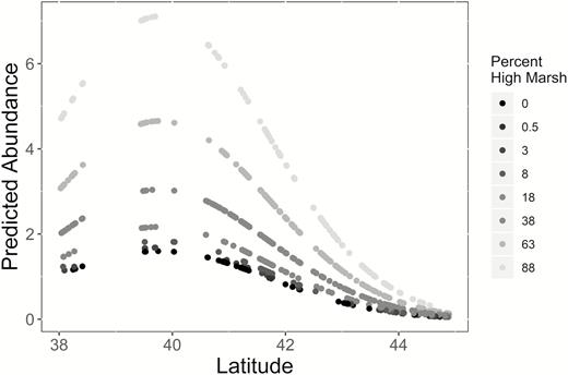
Predicted abundance of Saltmarsh Sparrows by latitude at 913 survey locations (represented by dots) across the entire breeding range surveyed during 2012. Predictions were based on the best-supported abundance model from our analysis, which included an interaction between angle to maximum horizon and distance to edge, along with additive effects of latitude (quadratic) and the percentage of high marsh habitat within 50 m of the survey point. Shading represents the median of each of 8 categories of percentage of area of high marsh vegetation within 50 m of the survey point. The model that generated predictions was corrected for detection probability (Table 1) and assumed mean values of distance to edge and angle to maximum horizon.
The abundance model that best fit our data overall included an interaction between angle to maximum horizon and distance to edge (Table 3, Figure 2, individual model weight >0.99). Further, all models that included angle to maximum horizon outcompeted all models that did not, and among the models with only one predictor of abundance, angle to maximum horizon outperformed all others (Table 3). All other models were not supported by our criteria, and patch area alone was the lowest ranked model other than the null model.
Model results, including ∆AIC, number of parameters (k), and model weight (wi) from models of abundance for Saltmarsh Sparrows surveyed during point counts from Maine to Maryland, April–July 2012. All models with interaction effects also include the respective additive terms.
| Model | k | ΔAIC a | wi |
|---|---|---|---|
| Angle to Maximum Horizon * Distance to Edge | 13 | 0.00 | 0.996 |
| Angle to Maximum Horizon * Patch Area | 13 | 11.29 | 0.004 |
| Angle to Maximum Horizon | 11 | 20.01 | <0.001 |
| Angle to Maximum Horizon + Maximum Horizon2 | 12 | 22.01 | <0.001 |
| Average Angle to Horizon | 11 | 39.55 | <0.001 |
| Patch Area * Distance to Edge | 13 | 57.73 | <0.001 |
| Distance to Edge | 11 | 90.37 | <0.001 |
| Patch Area | 11 | 99.20 | <0.001 |
| Null b | 6 | 254.08 | <0.001 |
a Lowest AIC score = 2,626.19. Log-likelihood of the top-ranked model is –1,300.096.
b Null model includes detection covariates from the top-ranked model for detection (Table 1), latitude (quadratic), and percent of high marsh habitat.
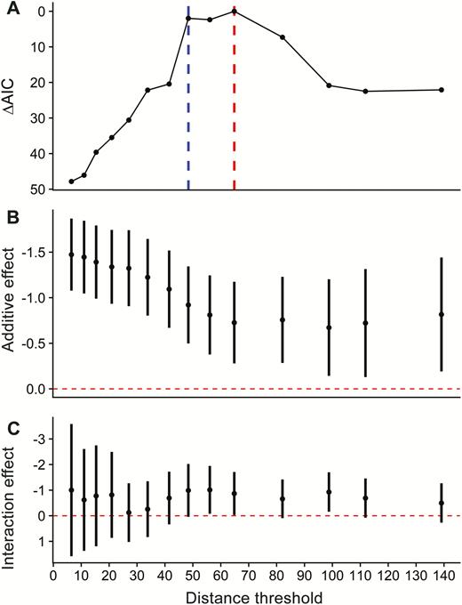
Results of post-hoc assessment exploring whether the effect of horizon angle on Saltmarsh Sparrow abundance exhibited a threshold as the distance from the nearest upland edge increased. (A) For each model, we recreated the structure of the best-supported abundance model but substituted a distance to edge threshold variable that represented whether each survey point fell beyond a particular distance. We evaluated change in model fit using ΔAIC as a function of increasing distance. The red vertical line represents the best-fit model, while the blue vertical line represents a second competitive (ΔAIC < 2.0) model. (B) Slope coefficients (β) for the additive effect of angle to maximum horizon on sparrow abundance. (C) Slope coefficients (β) for the interaction between angle to maximum horizon and distance to edge, where distance to edge was a binary variable indicating whether a point fell above or below each distance threshold. For panels B and C, error bars represent 95% CIs, and the red dashed horizontal line indicates no effect (slope = 0).
Saltmarsh Sparrow abundance was negatively associated with increased angle to the tallest object on the horizon (Table 2, Figure 3). When we held model parameters (distance to edge, latitude, and the percent cover of high marsh) constant at their mean values, the greatest predicted abundance of Saltmarsh Sparrows (3 birds per point survey location) occurred at an angle to the maximum horizon of 0°. At angle to maximum horizon values above 12.0°, predicted Saltmarsh Sparrow abundance fell below 1 bird per point. Our post-hoc analysis supported this same general pattern, suggesting it was relatively ubiquitous at a large geographic extent. Angle to maximum horizon was negatively correlated with abundance in all 6 ecoregions (Figure 3B); however, there were varying effect sizes and levels of precision among regions. For 4 of 6 ecoregions (regions 1, 2, 3, and 7; numbering is consistent with Wiest et al. 2016), the magnitude of the maximum horizon effect was similar or greater than the effect estimated from the full dataset (β range from –0.87 to –5.80). For 2 regions (4 and 5), the magnitude of the effect, while negative, was much closer to 0, and these regions occurred at the center of the species’ distribution where density was greatest (Figure 1). In 4 out of 6 regions, 95% CIs overlapped 0, while CIs did not overlap 0 for regions 2 and 5. We interpret the regional pattern in horizon effect size as evidence of a consistent general pattern for the species, with negative effects of maximum horizon peaking in low-density populations but being absent in high-density populations. Imprecision of the CIs likely results from a dramatically reduced sample size within each regional subset.
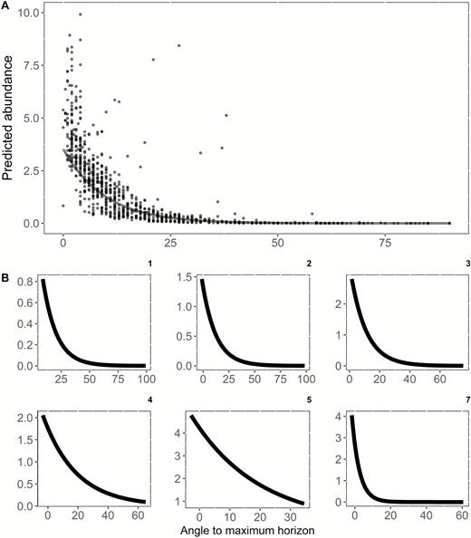
(A) Predicted abundance of Saltmarsh Sparrows as a function of the angle to the maximum horizon. Each point represents the predicted abundance for one of 913 survey locations from the overall model that includes an interaction between maximum horizon and distance to edge, along with additive effects of latitude (quadratic) and the percentage of high marsh habitat within 50 m of the survey point. The solid line reflects the predicted abundance at each point based solely on the additive effect of angle to maximum horizon (i.e. all other model effects held constant). A mean predicted abundance of one bird occurs at an angle of 21°. Sixteen outlier points (0.02% of all points) were omitted from the figure (but not the analysis) to better visualize the main pattern of the relationship. (B) Relationship between maximum horizon angle and predicted abundance for each of 6 subregional subsets of the data: (1) Coastal Maine, (2) Casco Bay to Cape Cod, (3) Southern New England, (4) Long Island, (5) Coastal New Jersey, (7) Coastal Delmarva; each described in detail by Wiest et al. (2016). Axis scaling for each subregion reflects the range of realized abundances and horizon angle estimates within that region.
Including the interaction between angle to maximum horizon and distance to edge greatly improved model performance. As distance to edge increased, the relative effect of angle to maximum horizon decreased. This is perhaps best illustrated by our post-hoc threshold analysis, which showed that model fit was maximized at a distance threshold of 64.8 m (Figure 2), with a similarly competitive threshold (∆AIC < 2.0) also occurring at 48.4 m (Table 4). Furthermore, the additive effect of angle to maximum horizon decreased as points were surveyed at greater distances from the edge until they were beyond this same distance threshold, and the interaction effect was only supported (95% CIs that do not overlap 0.0) near this distance threshold (Figure 2). Together these results suggest a biological threshold at a distance of ~50–70 m from the edge, below which the effect of angle to maximum horizon is a strong predictor of Saltmarsh Sparrow abundance, and above which the effect is reduced.
Model selection results, including ∆AIC and model weight (wi) from post-hoc models of abundance for Saltmarsh Sparrows surveyed during point counts from Maine to Maryland, April–July, 2012. This assessment tests whether different thresholds of distance to the upland edge model abundance better than distance as a continuous variable. For each model, we used a categorical variable that represented whether or not each survey point fell beyond a particular distance. We compared model performance among 18 different distance thresholds, defined by the 5% quantiles (between 10% and 95%) of the range of our measured distances. The full model included the variables of angle to maximum horizon, distance to edge, latitude (quadratic), and high marsh; all other models share this structure, but with distance to edge defined by each respective distance threshold.
| Distance threshold (m) | Quantile | ΔAIC a | wi |
|---|---|---|---|
| 64.8 | 55 | 0.00 | 0.59 |
| 48.4 | 45 | 1.99 | 0.22 |
| 56.1 | 50 | 2.37 | 0.18 |
| 82.1 | 60 | 7.31 | 0.02 |
| 41.5 | 40 | 20.43 | 0.00 |
| 98.8 | 65 | 20.87 | 0.00 |
| 139.1 | 75 | 22.10 | 0.00 |
| 33.8 | 35 | 22.16 | 0.00 |
| 111.9 | 70 | 22.51 | 0.00 |
| 27.0 | 30 | 30.57 | 0.00 |
| 170.1 | 80 | 32.59 | 0.00 |
| Full model b | NA | 34.55 | 0.00 |
| 20.9 | 25 | 35.49 | 0.00 |
| 15.3 | 20 | 39.61 | 0.00 |
| 11.0 | 15 | 46.07 | 0.00 |
| 222.5 | 85 | 47.23 | 0.00 |
| 6.5 | 10 | 47.84 | 0.00 |
| 312.1 | 90 | 57.01 | 0.00 |
| 539.0 | 95 | 58.10 | 0.00 |
a Lowest AIC score = 2,591.71. Log-likelihood of the top-ranked model is –1,282.857. All models include k = 13 parameters.
b Full model indicates the best-supported model from Table 3, which includes the best-supported structure for both detection and abundance terms and models distance to the upland edge as a continuous variable.
DISCUSSION
Understanding the relationship between habitat characteristics and abundance is integral to the effective conservation of species in decline. Based on our analyses, the angle to the maximum horizon (i.e. marsh openness) and distance to the marsh edge together approximate the environmental cues used by Saltmarsh Sparrows to select breeding sites, and were a better predictor of abundance than patch area. Whether these cues are based upon predator avoidance, perception of the amount of suitable habitat, or other not yet understood behavioral mechanisms, we found a clear pattern of greater abundance in more open patches. These results are consistent with a strategy in which birds avoid enclosed areas close to the habitat edge. The scale of edge avoidance we report here (within ~50–70 m of the edge) is similar to that reported for other grassland bird species (Winter et al. 2000, Renfrew et al. 2005). Fifty meters is a common threshold across many other studies of grassland edge effects as well (Paton 1994), and our results support the idea that at locations further than 70 m from the marsh edge, angle to the maximum horizon explained less variation in Saltmarsh Sparrow abundance than at locations closer to the marsh edge. It is possible that within this approximate distance, many open-country birds use the height of the horizon as a visual cue to assess habitat edge proximity. Because maximum horizon and distance to edge may both affect edge avoidance, they are important components to consider in conservation and restoration planning for this species.
When selecting marsh patches to protect, we suggest an additional focus on these 2 parameters rather than patch area alone, as our results indicate that even a small marsh with an open horizon may be more suitable for use by Saltmarsh Sparrows than a larger, more enclosed one. To increase the suitability of existing patches for Saltmarsh Sparrow use, techniques such as the removal of trees or other tall human structures near marsh edges may be productive both in the short term (by decreasing angle to maximum horizon) and the long term (by facilitating marsh migration inland). Management of maximum horizon height may mitigate the effect of edge proximity and promote colonization of marginal areas of salt marsh that are otherwise suitable but are presently avoided by Saltmarsh Sparrows.
These actions are especially noteworthy in the New England portion of the Saltmarsh Sparrow range, where marshes tend to be much smaller than those farther south and edge habitats therefore represent a larger proportion of the available regional marsh habitat. Importantly, however, we detected a significant impact of horizon in even the most southern ecoregion, where marshes are the largest (Figure 3). Interestingly, while our estimates of the impact of horizon were negative in all 6 ecoregions we examined, they were weakest in the range center where sparrow abundance is highest. Habitat filling, where individuals occupy less preferred environments as abundance increases, would explain the lower effect of horizon in the center of the range and the stronger effects at both the northern and southern range margins, although other mechanisms are certainly possible. Given the consistency of the direction of the estimates, however, we do not expect different underlying preferences for open habitats across the breeding range of this species.
We recognize that studies of habitat importance often focus on measures of reproductive performance such as nest abundance and success (Vickery and Hunter 1994, Meiman et al. 2012), whereas in this paper we focus exclusively on abundance. Saltmarsh Sparrows, particularly males, are known to establish breeding season home ranges in marshes where breeding does not occur, although this pattern is not well understood and marshes with confirmed nesting activity anecdotally exhibit higher sparrow densities. Measuring nest density and success is more time-intensive and costly than abundance surveys, making these types of data difficult for managers to obtain. Simple abundance surveys are a less resource-intensive method and offer a basic approximation of bird use of a patch, as nesting certainly cannot happen without presence. Further, many grassland species use openness as a habitat feature for nest site selection (van der Vliet et al. 2008, Keyel et al. 2013). However, our results suggest that future studies should explore evidence for effects of openness on nest site selection and reproductive success, which could produce valuable information about Saltmarsh Sparrows and other grassland passerines. Additionally, as our study is based upon 1 yr of abundance data, we could not evaluate the consequences of the relationships we observed to multi-year trends in sparrow abundance. Longer term studies of both adult abundance and reproductive success would be beneficial to strengthen the evidence for the patterns we observed.
Implications for Saltmarsh Management
North American saltmarsh condition and the overall area suitable for bird nesting is declining rapidly due to sea-level rise, coastal development, and other human activities (Field et al. 2017, Roberts et al. 2019), and immediate conservation action is necessary to mitigate further loss to this ecosystem. Protecting marshes is imperative for Saltmarsh Sparrows, which are currently being considered for listing by the U.S. Fish and Wildlife Service (U.S. Fish and Wildlife Service 2018) under the U.S. Endangered Species Act. Regardless of the outcome of that process, they are considered globally endangered, listed as endangered by the International Union for the Conservation of Nature (BirdLife International 2018), and listed as a Species of Greatest Conservation need in every U.S. state overlapping its breeding range (Delaware Department of Natural Resources and Environmental Control 2015, New Hampshire Fish and Game Department 2015, New York Department of Environmental Conservation 2015, Virginia Department of Game and Inland Fisheries 2015, Maine Department of Inland Fisheries and Wildlife 2016). As a result of this conservation status, numerous state and federal agencies are considering on-the-ground conservation actions to benefit the species (Atlantic Coast Joint Venture 2017).
Our findings imply that angle to maximum horizon and distance to edge should be considered when prioritizing marshes for sparrow conservation, rather than relying strictly on patch size. Marshes that seem suitable when considering patch size alone could, in reality, be made less so due to the presence of tall objects or the shape of the patch. Conversely, relatively small marshes may still be habitable if they are open. Marshes that maximize the interior area with an angle to the maximum horizon below 12° may be most beneficial to prioritize in order to protect the greatest number of individuals per hectare. Managers interested in prioritizing marshes for use by Saltmarsh Sparrows should assess the openness of marsh patches by finding the angle to the maximum horizon from the center of a marsh and by sampling within 50 m of the marsh edge to best evaluate the entire marsh patch. Keyel et al. (2012, 2013) also found an openness index based on angle to the horizon to be the best predictor of abundance for Bobolink; thus, further work is needed to explore the relationship between openness and perceived horizon in open-country birds.
Management experiments are also needed to test whether the removal of objects on marsh edges increase bird use of the marsh. Standing dead trees in areas where marshes are moving landward (e.g., Chesapeake Bay), for instance, is likely to prohibit use by Saltmarsh Sparrows despite shrinking suitable marsh to seaward. Tree removal has also been proposed as a potential method for speeding the conversion of upland areas into tidal marsh as sea levels rise (Field et al. 2016), which might be necessary to balance the ongoing losses of the high elevation marsh in which Saltmarsh Sparrows nest. Our results suggest that by removing tall trees, marsh areas that are presumably most resistant to sea-level rise (those nearest the upland edge) could be made more suitable for use by birds. Conversely, the areas of the marsh with the greatest current population densities (those furthest from the upland) are those most at risk from sea-level rise, and thus improvement of habitat suitability along the marsh edges may partially buffer population losses in the marsh interior.
Marsh openness and distance to edge together predict Saltmarsh Sparrow abundance better than marsh area and should be prioritized in marsh conservation efforts aimed at benefiting this declining species. Further, altering marsh characteristics along the upland edge may provide at least temporary refugia from sea-level rise by opening up currently unused, higher elevation habitats to sparrow occupancy.
ACKNOWLEDGMENTS
The authors and a large number of technicians collected and/or supervised data collection. Thanks to all SHARP collaborators, in particular landowners who allowed access to their properties and the National Wildlife Refuge staff of United States Fish and Wildlife Service (USFWS) Region 5 who provided numerous sources of in-kind logistical support. Of these, K. O’Brien, N. Pau, P. Castelli, E. King, S. Guiteras, H. Hanlon, A. Larsen, K. Holcomb, P. Denmon, and D. Curson deserve special mention. Thanks to S. Keyel and J. M. Reed for advice on measurement of openness. This is Maine Agricultural and Forest Experiment Station Publication Number #3734.. The research findings and conclusions in this article are solely those of the authors and do not necessarily represent the views of the USFWS.
Funding statement: Several sources provided funding for this research, including a Competitive State Wildlife Grant (U2-5-R-1) via the United States Fish and Wildlife Service and Federal Aid in Sportfish and Wildlife Restoration to the states of Delaware, Maryland, Connecticut, and Maine, the United States Fish and Wildlife Service (Region 5, Division of Natural Resources, National Wildlife Refuge System: P11AT00245, 50154-0-G004A), the United States Department of Agriculture (National Inst. of Food and Agriculture McIntire-Stennis Projects NH00068-M and ME0-21710), and the National Science Foundation (DEB-1340008, DGE-1144423).
Ethics statement: This study followed the standardized North American marsh bird monitoring protocol (Conway 2011). For this analysis we used no data from captured birds.
Author contributions: H.M., E.J.B., M.C., J.B.C., M.D.C., C.S.E., A.R.K., A.I.K., W.G.S., W.A.W., and B.J.O. contributed to the study idea and/or design. M.C., M.D.C., A.R.K., and W.A.W. collected the data. H.M., E.J.B., V.W., M.C., and B.J.O. analyzed the data. H.M., E.J.B., V.W., M.C., J.B.C., M.D.C., C.S.E., T.P.H., A.R.K., A.I.K., W.G.S., W.A.W., and B.J.O. wrote the manuscript.
Data depository: Analyses reported in this article can be reproduced using the data provided by Marshall et al. (2020).
