


Abstract
Observational pharmacoepidemiological studies using routinely collected healthcare data are increasingly being used in the field of nephrology to answer questions on the effectiveness and safety of medications. This review discusses a number of biases that may arise in such studies and proposes solutions to minimize them during the design or statistical analysis phase. We first describe designs to handle confounding by indication (e.g. active comparator design) and methods to investigate the influence of unmeasured confounding, such as the E-value, the use of negative control outcomes and control cohorts. We next discuss prevalent user and immortal time biases in pharmacoepidemiology research and how these can be prevented by focussing on incident users and applying either landmarking, using a time-varying exposure, or the cloning, censoring and weighting method. Lastly, we briefly discuss the common issues with missing data and misclassification bias. When these biases are properly accounted for, pharmacoepidemiological observational studies can provide valuable information for clinical practice.
INTRODUCTION
Pharmacoepidemiology uses epidemiological methods to study the use, therapeutic effects and risks of medications in large populations [1]. Due to the availability of routinely collected healthcare data from registries, electronic health records or claims databases, observational pharmacoepidemiological studies are increasingly being used to generate evidence to inform clinical practice. Our first review discussed the scope and research questions that are studied within the field of pharmacoepidemiology and described the strengths and caveats of the most commonly used study designs to answer such questions [2]. We now focus on the most common biases that may occur when using observational data to study the causal effects of medication on health outcomes. We will attempt to offer possible solutions in the design or statistical analysis to prevent or minimize such biases. The review is intended as an introduction to the field for those who wish to critically appraise pharmacoepidemiological studies or conduct such studies.
CONFOUNDING BY INDICATION
Confounding by indication is a threat to any observational study assessing the effects of medications, as treatment is not randomly assigned to patients. Confounding by indication arises when the indications for treatment, such as age and comorbidities, are also related to the outcome under study [3]. For example, treatment is generally given to those with a worse prognosis. The reverse may also occur, as when newly introduced drugs are first prescribed to individuals perceived as healthier and who may be more likely to tolerate them [4]. Both situations lead to an uneven distribution of prognostic factors between treatment groups, which biases a direct comparison. Take the case shown in Figure 1A, where albuminuria is a confounder for the effect of angiotensin-converting enzyme inhibitor (ACEi) treatment on kidney replacement therapy: individuals with albuminuria are more likely to be prescribed ACEis and albuminuria is also an independent risk factor for kidney replacement therapy. Unknown or unmeasured confounders for the treatment–outcome relationship may also be present, such as smoking (if this variable has not been measured and we assume that smoking can affect the decision to start ACEi therapy as well as the outcome).
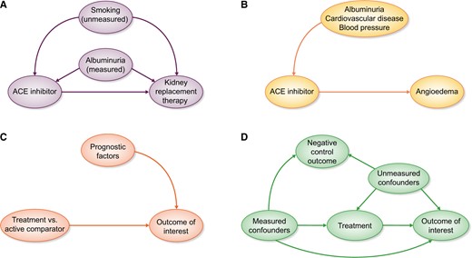
(A) Confounding by indication arises when prognostic factors for the outcome also influence the decision to start treatment. Some confounders may be measured, which can be adjusted for in the analysis, whereas others are unmeasured, leading to residual confounding. (B) When unintended outcomes are studied, less confounding by indication will be present. The indications for ACEi treatment likely do not increase the risk for the outcome angioedema. (C) An ideal active comparator has similar indications as the medication under study, thereby decreasing confounding by indication. Ideally the active comparator should have no influence on the outcome. (D) Negative control outcomes need to have similar measured and unmeasured confounders as the treatment–outcome relationship under study. Furthermore, treatment should not have an influence on the negative control outcome.
Addressing confounding by indication when designing a pharmacoepidemiological study
When designing observational studies to investigate medication effectiveness or safety we should be aware that some research questions will be more susceptible to confounding than others. Confounding will generally play a larger role when studying the beneficial or ‘intended’ effects of treatments, as the indications for treatment are very likely to be related to the prognosis of the patient [5]. On the other hand, if the outcome is completely unrelated to the indications for treatment, such as when studying rare side effects or ‘unintended’ effects, no confounding would be present [6]. A classic example is the relationship between ACEis and angioedema. Patient characteristics that determine treatment status (e.g. cardiovascular risk, albuminuria and blood pressure) are unlikely to be associated with the outcome angioedema. Consequently the arrow from treatment indication to outcome will be absent and confounding by indication will not be an issue (Figure 1B).
Applying an active comparator design may also decrease confounding by indication [7]. In an active comparator design, the medication of interest is compared with another drug that has similar indications rather than a nonuser group. The more exchangeable the active comparator is for the medication of interest, the lower the risk for potential confounding will be. After all, if both treatment groups have identical treatment indications (both measured and unmeasured characteristics), there would be no arrow from indication to treatment and confounding by indication is removed (Figure 1C) [8]. A recent example for applying an active comparator design investigated whether proton pump inhibitors (PPIs) increased the risk of chronic kidney disease (CKD) [9]. Comparing PPI users with nonusers may suffer from unmeasured confounding, since nonusers are generally healthier and not all confounders may have been captured in the dataset and adjusted for. Histamine-2 receptor antagonists are prescribed for similar indications as PPIs. Users of these two medications may be more similar regarding comorbidities, medication use and other unmeasured variables.
Adjusting for confounding during the statistical analysis
Selecting an appropriate set of confounders to adjust for is critical when conducting pharmacoepidemiological studies [10]. In general, it is not recommended to use data-driven variable selection methods to identify confounders, such as only retaining statistically significant confounders or including variables that change the regression coefficient of the treatment variable [11–13]. Such data-driven approaches can lead to bias if they adjust for mediators (i.e. variables in the causal pathway between exposure and outcome) [11], colliders (i.e. a variable caused by both treatment and outcome) [14, 15] and instrumental variables (i.e. variables strongly related to the exposure but not to the outcome) [16], although some sophisticated statistical covariate selection methods are currently under development [10, 17–19]. Instead, we suggest making directed acyclic graphs (DAGs) and selecting confounders based on subject-matter knowledge and biological plausibility [20, 21]. Since DAGs rely on prior knowledge and assumed causal effects, they do not tell whether these assumptions are correct. Different researchers can have different views on which factor causes the other and this may result in different choices regarding which confounders to adjust for. DAGs can aid in this discussion by making the causal assumptions explicit in a graphical manner.
Once the confounders have been selected, various methods can be used to adjust for confounding. These include, for instance, multivariable regression, standardization and propensity score methods (propensity score matching, weighting, stratification or adjustment). In the time-fixed setting (i.e. when treatment is only measured once), all methods generally suffice to adjust for measured confounding, although the interpretation of the effect estimate may differ depending on the method, and some methods are preferred in specific settings [22–25]. A thorough discussion on the merits and caveats of multivariable regression and propensity score methods can be found elsewhere [26]. Nonetheless, in the setting of time-varying treatments (i.e. when treatment is received at multiple timepoints and changes over time) and time-varying confounding, methods based on weighting or standardization are required to give unbiased estimates if the confounders themselves are affected by treatment [27]. It should be kept in mind that all statistical methods mentioned above can only adjust for measured confounders, but not for unmeasured confounders as is sometimes claimed [28], unless the unmeasured confounders are correlated with the variables that are adjusted for [29, 30].
Assessing the impact of unmeasured confounding
Although the possibility of residual or unmeasured confounding in observational analyses can never be fully eliminated, a number of steps can be taken to alleviate concerns and strengthen inferences. In this section we will elaborate on conducting sensitivity analyses to obtain corrected effect estimates, calculating the E-value and conducting negative control outcome and control group analyses.
First and foremost, as many confounders as possible need to be identified and adjusted for by using appropriate statistical methods. However, if known confounders (e.g. albuminuria or smoking) have not been measured, corrected effect estimates can be calculated in quantitative bias analyses [31–34]. This requires an input of the assumed association between confounder and exposure and between confounder and outcome and the prevalence of the confounder in the population. These numbers can be based on previous studies and can be varied over a range of values to give an indication of how sensitive the estimated treatment effect is to unmeasured confounding [35]. If results lead to the same conclusion over a wide range of relevant scenarios, then the plausibility of the estimated treatment effect will increase.
Alternatively, one can estimate how strong the unmeasured confounding would need to be to completely explain away a certain effect estimate. The E-value has recently been introduced as an easily implemented tool for these purposes [36–39]. The E-value is defined as ‘the minimum strength of association … that an unmeasured confounder would need to have with both the treatment and the outcome to fully explain away a specific treatment-outcome association, conditional on the measured covariates’ [36]. As an example, researchers investigated whether the use of sodium polystyrene sulphonate (SPS) to treat hyperkalaemia increased the risk of severe adverse gastrointestinal events in persons with CKD [40]. After adjustment for measured confounding, the initiation of SPS was associated with a 1.25 (95% confidence interval 1.05–1.49) higher risk of severe gastrointestinal events. The corresponding E-value for this hazard ratio was 1.80, meaning that an unmeasured confounder would need to be associated with both SPS initiation and severe gastrointestinal events by a hazard ratio of 1.80 to decrease the point estimate from 1.25 to 1.00. What constitutes a large E-value is context-specific and depends on the specific research question under study, the effect size of the exposure and the hazard ratios of the confounders that have already been adjusted for [38, 41, 42]. Easily implemented online calculators are available to conduct the discussed sensitivity analyses [37, 43, 44].
For certain research questions ‘negative control outcomes’ can be used to provide guidance about the presence and magnitude of unmeasured confounding in observational studies [45]. A negative control outcome is an outcome that is not influenced by the treatment of interest but shares the same set of measured and unmeasured confounders as the treatment of interest–outcome relationship (Figure 1D) [46]. Hence we would not expect to find an association between the exposure of interest and the negative control outcome. As an example, one may be concerned that the unmeasured variables body mass index and smoking bias the results of a study investigating the association between a cardiovascular drug and the risk of cardiovascular-related mortality. However, we would not expect the cardiovascular drug to also lower noncardiovascular mortality. If we unexpectedly found a lower risk of the negative control outcome noncardiovascular mortality among treated individuals, this might be an indication of residual confounding or other sources of bias. In addition to the previously mentioned assumptions, the negative control outcome should occur with a frequency similar to the primary study outcome to ensure enough power to reject the null hypothesis of no association. If such assumptions are not met, this may erroneously lead to the conclusion that no unmeasured confounding is present [47].
Similarly, one can test whether associations are as expected in a certain ‘control group’. The direction of the expected association (either a positive, negative or null association) can be based on physiologic mechanisms or evidence from randomized trials [48]. For example, Weir et al. [49] hypothesized that users of high-dialysable β-blocker would have an increased risk of mortality compared with users of low-dialysable β-blocker, due to loss of high-dialysable β-blocker in the dialysate. To strengthen their inferences, a control group of patients with CKD Stage G4–5 was constructed in which a similar effectiveness of high- and low-dialysable β-blockers was expected and subsequently demonstrated. Control groups can also strengthen inferences by showing similar results between observational studies and randomized trials. We recently evaluated the effectiveness of β-blockers in patients with heart failure and advanced CKD, a population that was excluded from landmark heart failure trials [50]. A positive control group including heart failure patients with moderate CKD showed a benefit similar to that observed in moderate CKD patients from randomized trials. This positive control analysis further supported a causal explanation for the results in the advanced CKD cohort.
PREVALENT USER AND IMMORTAL TIME BIASES
We now discuss two types of biases that often occur in pharmacoepidemiological studies but which can and should be avoided by adhering to a simple principle: aligning the start of the follow-up with the start of exposure.
Prevalent user bias
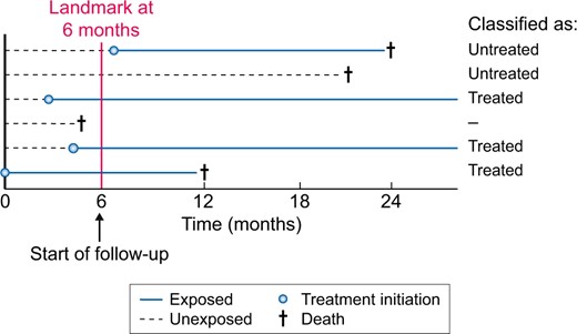
When we want to assess the effectiveness of initiating a drug, it is recommended to include incident medication users instead of prevalent users [51, 52]. In a new-user or incident-user design, only individuals who ‘initiate’ the medication of interest are studied and followed from the date of treatment initiation. Therefore the start of follow-up and start of treatment will align and all events that occur after drug initiation are captured [53, 54]. In contrast, prevalent-user designs include individuals who initiated the exposure of interest some time ‘before’ the start of follow-up (Figure 2A). Comparing prevalent users to nonusers may introduce selection bias since individuals who died before enrolment cannot, per definition, be included in the analysis and events occurring shortly after drug initiation are not observed [55, 56]. To better understand why this selection bias arises, we give a real-world example. Suppose we conducted a randomized trial and found that a certain medication increased the risk of myocardial infarction with a hazard ratio of 1.24. We now reanalyse the data by starting follow-up at 2 years after randomization. Hence we only count the myocardial infarctions that occurred after 2 years of follow-up. By doing so we also exclude all individuals who died or experienced myocardial infarction in the first 2 years after randomization. This new analysis paradoxically (rather erroneously) shows that the medication ‘lowers’ the risk of myocardial infarction. Since the medication increases the risk of myocardial infarction, the treatment arm will be progressively depleted of patients most susceptible to the event [57]. After 2 years the treated group will only consist of survivors who likely do not have other risk factors for myocardial infarction. Therefore, comparing these survivors in the treatment group with those remaining in the control group leads to an unfair advantage for the treatment group. Prevalent-user bias is one of the proposed reasons why postmenopausal hormone therapy appeared protective for coronary heart disease in observational studies but was actually harmful when subsequent randomized trials were conducted [58, 59]. Besides the fact that the effect estimates from a prevalent-user design are biased, they also do not inform decision making, as the decision to start the treatment was already made in the past. Studies applying a prevalent-user design do not answer the relevant question of whether treatment should be initiated. The results of such a study can only tell you that if a person has survived on treatment for this long, we know he is not susceptible to the event, which gives him a better prognosis than untreated individuals who are still susceptible.

Graphical visualization of (A) prevalent-user bias and (B) immortal time bias when setting up the start of follow-up in a study. For prevalent-user bias, the start of follow-up occurs after treatment initiation, whereas for immortal time bias, the start of follow-up occurs before treatment initiation. These biases can be prevented by aligning the start of follow-up with the start of exposure.
Immortal time bias
Immortal time bias occurs when patients are classified into treatment groups at baseline based on the treatment they take ‘after’ baseline (Figure 2B) [60, 61]. This leads to a period of time (i.e. immortal time) between baseline and the start of treatment where no deaths can occur in the treatment group, thereby biasing results in favour of the treatment group. As an example, a pharmacoepidemiological study investigated the long-term effects of metformin use versus no metformin use on mortality and end-stage kidney disease [62]. In this study, follow-up started when patients had a first creatinine measurement, but patients were classified as metformin users when they had been prescribed metformin for >90 days ‘during’ the follow-up period. Using postbaseline information on metformin use to classify patients at baseline into the metformin group leads to an unfair survival advantage for metformin users [63]. Imagine that all individuals in the metformin group started medication only after 5 years of follow-up. By definition, no deaths would then occur in the metformin group during the first 5 years of follow-up. After all, individuals who have an event prior to taking up treatment would be classified as untreated. Using postbaseline information for exposure classification thus results in immortal time bias [60, 64]. To what extent the effect estimate is biased depends on the total amount of follow-up that is erroneously misclassified under the metformin group. The bias will increase with a larger proportion of exposed study participants, a longer period of time between start of follow-up and initiation of treatment and a longer duration of follow-up [65].
POTENTIAL SOLUTIONS TO MITIGATE IMMORTAL TIME BIAS
We now discuss three designs that could be applied to avoid immortal time bias: landmarking, using a time-varying exposure and using treatment strategies with grace periods. Other more complex solutions exist but are outside the scope of this review and are discussed elsewhere [66–68].
In pharmacoepidemiological studies we are often interested in the effects of initiating medication on a particular outcome after a certain event has occurred. A recent clinical example is the effect of initiating renin–angiotensin system inhibitors (RASis) on mortality and recurrent acute kidney injury (AKI) after AKI [69–71]. When using routinely collected healthcare data to study such questions, it is often difficult to assign individuals to the correct exposure groups: individuals become eligible for inclusion in our study immediately after the AKI event and follow-up will start at that moment. However, directly after the AKI event, all individuals will likely be unexposed in our dataset, as individuals will gradually initiate therapy during follow-up. We cannot classify individuals in exposure groups based on postbaseline information, as this will lead to immortal time bias. The easiest solution is to move the baseline of our study from the date of the AKI event to a later time, e.g. 6 months after the AKI event. Our follow-up will therefore start at 6 months after the index AKI event (Figure 3) [72–74]. This method is called landmarking and was recently applied by Brar et al. [69] for this particular research question. In the landmarking method, all individuals who died or developed the outcome between the AKI event and the newly chosen start of follow-up (i.e. 6 months after AKI) are excluded; those who initiate treatment during this period are considered exposed and those who do not initiate treatment during this period are considered unexposed. Although landmarking prevents immortal time bias, the attentive reader will have noted that it can introduce prevalent-user bias, which was discussed in the previous section.
Design of a landmark analysis to prevent immortal time bias. In the landmark analysis, follow-up starts at a chosen time period after a certain event, in this example at 6 months. Hence all individuals that died before Month 6 are excluded from the analysis (Individual 4). Individuals are then classified according to exposure status in the first 6 months. Individuals 3, 5 and 6 are therefore considered treated, whereas Individuals 1 and 2 are considered untreated.
The next solution that prevents immortal time bias and allows starting follow-up immediately after the event has occurred is the use of a ‘time-varying exposure’ (Figure 4). When using a time-varying exposure, individuals are allowed to switch exposure status from untreated to treated at the time of treatment initiation. Hence individuals will contribute person-time to the unexposed group before treatment initiation and to the exposed group after treatment initiation. This ensures that the time between the start of follow-up and initiation of treatment will be correctly assigned to the nonusers. For example, Hsu et al. [70] used a time-varying exposure to study the effect of RASis after AKI on the risk of recurrent AKI. As previously mentioned, using a time-varying exposure involves time-varying confounding. When these confounders are also influenced by prior treatment, using standard methods such as multivariable regression may not be appropriate. Instead, methods such as marginal structural models that are based on inverse probability weighting can be used [27, 75]. Applying these methods, the authors found that new use of RASi therapy was not associated with an increased risk of recurrent AKI.
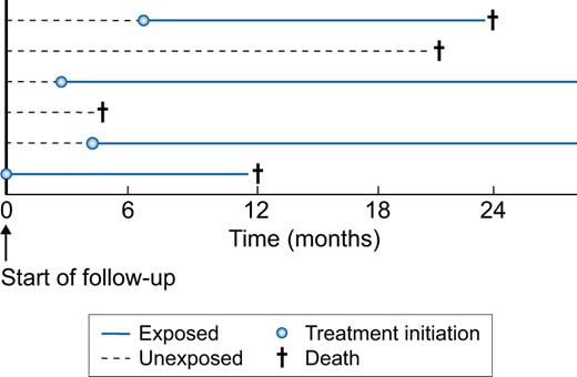
Analysis using a time-varying exposure to prevent immortal time bias. In a time-varying design, treatment status is allowed to change from unexposed to exposed at the moment of treatment initiation. This method allows the start of follow-up directly after the event has occurred and also does not exclude individuals. For example, Individual 1 is considered unexposed for the first 7 months of follow-up, but after 7 months will contribute to the exposed group. In the setting of time-varying exposures, time-varying confounding will be present too, which sometimes requires more advanced methods, such as marginal structural models, to obtain unbiased effect estimates.
Lastly, we might be interested in comparing treatment strategies that include a grace period [76]. For example, we could compare the strategies ‘initiate an ACEi within 6 months after the AKI event’ versus ‘do not initiate an ACEi within 6 months after the AKI event’. The length of the grace period depends on what is commonly done in clinical practice. These treatment strategies with a grace period can be investigated by using a three-step method based on cloning, censoring and weighting (Figure 5). Briefly, each individual is duplicated so that there are two copies of each individual in the dataset. Each copy is then assigned to one of the treatment strategies. In the second step, the copies are censored if and when their observed treatment no longer adheres to their assigned treatment strategy. Since this censoring is likely to be informative, the third step applies inverse probability weighting to correct for this. Bootstrapping can be used to take into account the cloning and weighting to obtain valid confidence intervals. An advantage of using treatment strategies with grace periods is that a wide range of questions can be answered, including questions on the duration of treatment and dynamic treatment strategies (e.g. when should treatment be initiated) [76, 77]. However, this method requires that detailed longitudinal data are present to adequately adjust for the informative censoring. The three methods of landmarking, time-varying exposure and treatment strategies with grace periods are contrasted in Table 1 and graphically depicted in Figures 3–5.
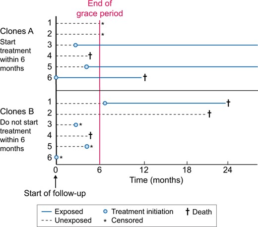
Design of a study using treatment strategies with a grace period based on cloning, censoring and weighting. Another method is comparing treatment strategies that include a grace period. Each individual is duplicated and assigned to one of two treatment strategies. In this example, Clones 1a–6a follow the strategy ‘initiate ACEi within 6 months’, whereas Clones 1b–6b follow the strategy ‘do not initiate ACEi within 6 months’. Note that Copies 1a and 1b represent the same individual. Since Copy 1a is assigned to initiating within 6 months, he is censored after Month 6, as he did not initiate treatment. The censoring is likely to be informative and inverse probability weighting is required to adjust for this.
Different methods to address immortal time bias in pharmacoepidemiological analyses
| Characteristics | Landmark analysis | Time-varying exposure | Cloning, censoring and weighting |
|---|---|---|---|
| Immortal time bias | No | No | No |
| Start of follow-up | At landmark | At event | At event |
| Causal effect | Initiating versus not initiating at x months after event (landmark), conditional on having survived until landmarka | Initiating and always using versus never using (marginal structural model) | Initiating within x months versus not initiating within x months after event |
| Prevalent user bias | Possible | No | No |
| Results apply to | Individuals surviving until landmark | All individuals | All individuals |
| Baseline confounding | Yes | Yes | Nob |
| Time-varying exposure | No | Yes | No |
| Time-varying confounding | No | Yes | No |
| Informative censoring | No | No | Yes |
| G-methodsc required | No | Sometimes (if confounder is influenced by prior treatment) | Yes (inverse probability weighting) |
This is often how the effect estimate from a landmark analysis is interpreted. However, the landmark analysis conditions on surviving until a certain timepoint and classifies individuals into treatment groups based on past information, thereby possibly introducing prevalent-user bias.
Due to the cloning, at baseline each individual will appear in both treatment arms. Hence no baseline confounding will be present.
Methods based on standardization or inverse probability weightings, such as the G-formula or marginal structural models.
MISSING DATA AND MISCLASSIFICATION
We now briefly discuss the implications of missing data and misclassification for bias and possible solutions. Although these two sources of bias are a common issue in pharmacoepidemiological studies, they are often less emphasized compared with confounding.
Missing data
We usually aim to adjust for as many confounders as possible in our analysis, including available laboratory tests (e.g. albuminuria, potassium) and clinical variables (e.g. blood pressure, BMI) that are indications for treatment. However, it is not unusual that a large proportion of these values are missing in routinely collected data. For example, in an analysis using data from the Swedish Renal Registry, baseline potassium and albuminuria:creatinine ratio measurements were missing in 32 and 41% of patients, respectively [78]. In such situations, researchers often perform a complete case analysis by restricting it to individuals with both measurements available. However, this may lead to a drastic reduction in power and often also bias [79, 80]. Methods such as multiple imputation are therefore recommended and are available in most software packages. These methods can reduce these biases even with large proportions of missing data (up to 90%) if data are missing at random or missing completely at random, sufficient auxiliary information is available and the imputation model is properly specified [81]. It is therefore important to discuss the reasons for missingness and the plausibility of the missing-at-random assumption. In the above example, the researchers explained that although albuminuria and potassium values were measured in clinical practice, they were not among the list of mandatory laboratory markers that needed to be reported to the Swedish Renal Registry. Thus some clinicians took the time to report those lab tests and others did not, a decision that could be assumed to be random. Furthermore, the authors showed that clinical characteristics were similar for individuals with and without missing data, thereby making the missing-at-random assumption plausible. More information on the different types of missingness [79, 80], in what situations complete case analysis leads to unbiased results [82] and tutorials to implement multiple imputations can be found elsewhere [83].
Misclassification
Although misclassification will be present in nearly every study, it may be especially important when using routinely collected healthcare data [84]. For instance, misclassification may occur when using International Classification of Diseases, Tenth Revision (ICD-10) codes to ascertain the occurrence of CKD or AKI, as these are not always coded in clinical practice and many patients are unaware of their disease [85–87]. When an AKI diagnosis based on ICD coding is used as an outcome, differential misclassification will arise when doctors are more aware or more likely to encode AKI if certain drugs are prescribed. Basing kidney outcomes on biochemical criteria may sometimes mitigate such biases but can also introduce bias when creatinine testing is more often directed towards sicker patients or patients at risk of CKD progression. Misclassification of comorbidities may be a significant concern in routinely collected data since the absence of a diagnosis (recording) is often considered to indicate absence of the comorbidity. Residual confounding may occur when confounders are misclassified and the direction can be both away or towards a null effect [84]. Misclassification influences study results in ways that are often not anticipated, and simple heuristics about the impact of misclassification (towards the null or not) are often incorrect [88, 89]. Many correction methods for misclassification exist, but these require information about its magnitude and structure (i.e. dependent, nondependent, differential and nondifferential) [90–93]. As such information is often not available in electronic databases, sensitivity analyses similar to those for unmeasured confounding can be performed to estimate the influence of misclassification on results [33, 94].
CONCLUSION
Pharmacoepidemiological studies are increasingly being used to answer causal questions on the effectiveness and safety of medications in order to inform clinical decision making. In this review we discussed the most important biases that commonly occur in such studies. We also reviewed methods to account for these biases, which are summarized in Table 2. Researchers can and should prevent problems arising from immortal time and prevalent-user biases in their study design. Confounding by indication bias can be tackled by using an active comparator design and adequately adjusting for confounders. When concerns remain about confounding or misclassification, quantifying their impact on effect estimates is recommended. When these principles are correctly applied, pharmacoepidemiological observational studies can provide valuable information for clinical practice.
Potential biases in pharmacoepidemiological studies and proposed solutions
| Potential biases | Example of how biases may arise | Possible solutions and recommendations |
|---|---|---|
| Confounding by indication | Confounding by indication arises when prognostic factors for the outcome are also an indication for initiating treatment. Unmeasured/residual confounding arises when confounders are not adjusted for, either if they are not measured in the dataset or if they are unknown. Time-varying confounding occurs when investigating time-varying exposures. When the confounder is influenced by past treatment, conventional methods to control for confounding will be biased. | Research question: Unintended medication effects (e.g. rare side effects) may be less susceptible to confounding by indication than intended medication effects. Design: Active comparator designs may decrease confounding bias if medication is given for similar indications. Statistical methods: Multivariable regression, standardization or propensity score methods (matching, weighting, stratification and adjustment) can be used to control for measured confounding. Propensity score methods may have a number of advantages compared with regression, such as the ability to check if balance in confounders has been achieved. In the presence of time-varying confounding that is influenced by treatment, conventional methods lead to bias and the so-called G-methods are required. After analysis: The impact of unmeasured confounding on effect estimates can be investigated in simulation analyses. Negative control outcomes may investigate whether unmeasured confounders bias effect estimates. |
| Prevalent-user bias | Comparing ever-users versus never-users. Including individuals after they initiate treatment will miss early outcome events and exclude those that died (depletion of susceptibles). | Prevalent-user bias can and should be prevented by aligning initiation of treatment with the start of follow-up; include new users of treatment. Exclude prevalent users, e.g. those with drug prescription in 12 months prior to inclusion. |
| Immortal time bias | Classifying individuals in treatment groups based on future information not present at the start of follow-up. A period of time is created for the treated group during which the outcome cannot occur. | Immortal time bias can and should be prevented by aligning initiation of treatment with the start of follow-up. Do not use information after the start of follow-up to classify individuals into exposure groups. Landmarking, time-varying exposure and the cloning, censoring and weighting method. |
| Missing data | Routinely collected healthcare data are prone to missing data. In multivariable analyses, individuals with missing confounder data will be excluded. Complete case analysis often leads to bias when data are not missing completely at random, but a number of exceptions exist. | Multiple imputations can be used to decrease bias and increase precision, even with large proportions of missing data (up to 90%) if data are missing at random or missing completely at random and the imputation model is properly specified. Discuss the missing data mechanism and the plausibility of the missing (completely)-at-random assumption |
| Misclassification | Misclassification of the outcome may occur when outcomes are differentially ascertained depending on treatment status. Misclassification of confounders may lead to residual confounding. | The impact of misclassification on the estimated effect size can be quantified in sensitivity analyses. Online tools are available to implement these methods. When external data are available, regression calibration, multiple imputations for measurement error or propensity score calibration can be used. |
FUNDING
This work was supported by the Swedish Research Council (grant 2019-01059) and the Swedish Heart and Lung Foundation.
CONFLICT OF INTEREST STATEMENT
None declared.
REFERENCES
Applying quantitative bias analysis to epidemiologic data. https://sites.google.com/site/biasanalysis/ (1 September 2020, date last accessed)


Comments