


Abstract
During tactile sensation by rodents, whisker movements across surfaces generate complex whisker motions, including discrete, transient stick–slip events, which carry information about surface properties. The characteristics of these events and how the brain encodes this tactile information remain enigmatic. We found that cortical neurons show a mixture of synchronized and nontemporally correlated spikes in their tactile responses. Synchronous spikes convey the magnitude of stick–slip events by numerous aspects of temporal coding. These spikes show preferential selectivity for kinetic and kinematic whisker motion. By contrast, asynchronous spikes in each neuron convey the magnitude of stick–slip events by their discharge rates, response probability, and interspike intervals. We further show that the differentiation between these two types of activity is highly dependent on the magnitude of stick–slip events and stimulus and response history. These results suggest that cortical neurons transmit multiple components of tactile information through numerous coding strategies.
Introduction
Rodents use their whiskers to detect and distinguish a variety of tactile features in their environment (Brecht et al. 1997; Kleinfeld et al. 2006), including object position (Mehta et al. 2007; Knutsen and Ahissar 2009; Kleinfeld and Deschenes 2011), shape (Brecht et al. 1997; Harvey et al. 2001), aperture and gap width (Krupa et al. 2001), and textures (Carvell and Simons 1990; Diamond, von Heimendahl, Knutsen, et al. 2008; Lottem and Azouz 2009; Diamond 2010; Jadhav and Feldman 2010; Morita et al. 2011; Kuruppath et al. 2014). The active and receptive interactions between the whiskers, given these biomechanical properties (Hartmann et al. 2003; Towal et al. 2011; Hires et al. 2013) and the environment, lead to frictional movement and induce whisker bends, vibrations, and brief, discrete high-velocity, high-acceleration micromotions called stick–slip events (SSE) (Diamond, von Heimendahl, and Arabzadeh 2008; Wolfe et al. 2008; Lottem and Azouz 2009; O'Connor et al. 2010; Zuo et al. 2011; Chen et al. 2015; Campagner et al. 2018). These events are a prominent feature of whisker-surface interactions in anesthetized and awake rats. Studies in recent years have shown that kinematic profiles of SSE carry texture information (Ritt et al. 2008; Wolfe et al. 2008) and are readily encoded by neurons on the ascending tactile pathway (Pinto et al. 2000; Jones et al. 2004; Arabzadeh et al. 2005; Jadhav et al. 2009; Jadhav and Feldman 2010; Stuttgen and Schwarz 2010; Waiblinger et al. 2013; Waiblinger, Brugger, Whitmire, et al. 2015; Allitt et al. 2017). These events evoke low-probability responses in the primary somatosensory (S1) cortex (Simons 1978; Pinto et al. 2000; Kerr et al. 2007; Stuttgen and Schwarz 2008; Crochet et al. 2011), which are related to SSE characteristics (Jadhav et al. 2009; Isett et al. 2018). Thus, sensory coding in S1 is assumed to be sparse (Brecht 2007), and sparse activation of small numbers of S1 neurons is perceptually and behaviorally relevant (Houweling and Brecht 2008; Huber et al. 2008; Ritt et al. 2008; Wolfe et al. 2008; Waiblinger, Brugger, and Schwarz 2015; Waiblinger, Brugger, Whitmire, et al. 2015; Isett et al. 2018; Zuo and Diamond 2019a).
How does the cortex make this sparse firing matter? The encoding of sensory stimuli has been studied extensively across species and sensory systems. Nevertheless, several open questions remain, particularly regarding the coding of complex stimuli. Although there is a longstanding debate on rate versus temporal coding (Theunissen and Miller 1995; Shadlen and Newsome 1998; deCharms and Zador 2000), recent studies in several sensory and motor systems have found evidence that the simultaneous usage of both types of encoding represents different stimulus features (Riehle et al. 1997; Panzeri and Diamond 2010; Ainsworth et al. 2012; Gire et al. 2013; Harvey et al. 2013; Wohrer et al. 2013; Saal and Bensmaia 2014; Ranjbar-Slamloo and Arabzadeh 2019). The simultaneous usage of several types of encoding is known as multiplexing and consists of combining different stimulus properties by distinct neuronal response features. Numerous studies have shown that this type of coding is prevalent (Riehle et al. 1997; Dan et al. 1998; Friedrich et al. 2004; Biederlack et al. 2006; Masuda 2006; Blumhagen et al. 2011; Harvey et al. 2013; Akam and Kullmann 2014; Metzen et al. 2015; Zuo et al. 2015; Hong et al. 2016; Isett et al. 2018; Lankarany et al. 2019).
We found that an essential feature of sensory-evoked activity in the barrel cortex is temporal coding. This coding is expressed in the temporal coincidence of a subset of the spikes in the neuronal population, thus forming a dynamically and functionally relevant subnetwork (Palm 1990; Hebb et al. 1994; Singer 1999; Lestienne 2001; Womelsdorf and Fries 2007; Cohen and Kohn 2011). Over the last several years, it has been shown that neuronal synchrony is prevalent in the barrel cortex of anesthetized and awake rodents (Zhang and Alloway 2004, 2006). This synchrony is present in the membrane potentials in neurons with similar sensory response dynamics, which were shown to be highly correlated during active touch, thus pointing to a specific synchronization of functional subnetworks (Ferezou et al. 2007; Poulet and Petersen 2008; Crochet et al. 2011). Moreover, the coding of SSE may be mediated by increases in the joint firing rate in S1 (Jadhav et al. 2009). To examine the hypothesis that multiplexed coding is involved in transmitting tactile information, we simultaneously measured whisker micromotion in response to textured surfaces and multineural activity in S1 in lightly anesthetized rats. Our findings suggest that there are potentially multiple complementary tactile information channels that may operate simultaneously within the same spike train (Harvey et al. 2013; Zuo et al. 2015).
Materials and Methods
Animals and Surgery
Sprague Dawley rats (250–320 g) were initially anesthetized with ketamine (100 mg/kg, i.p.; Ketaset; Fort Dodge Animal Health, Fort Dodge, IA) and acepromazine maleate (1 mg/kg, i.p; PromAce; Fort Dodge Animal Health). After tracheotomy, a short (1.5 cm) metal cannula [outer diameter (o.d.), 2 mm; inner diameter (i.d.), 1.5 mm] was inserted into the trachea. The rats were placed in a standard stereotaxic device. Body temperature was kept at 37.0 ± 0.1 °C using a heating blanket and a rectal thermometer (TC-1000; CWE, Ardmore, PA). Anesthesia was maintained, using a mixture of halothane (0.5–1.5%) and air, by means of artificial respiration at a rate of 100–115 breaths/min while monitoring the levels of end-tidal CO2 and heart rate. Anesthesia was maintained using a mixture of halothane (0.5–1.5%) and air using artificial respiration at a rate of 100–115 breaths/min while monitoring the levels of end-tidal CO2 and heart rate. Anesthesia was monitored by heart rate (250–450 beats/min), eyelid reflex, pinch withdrawal, and vibrissal movements. Halothane concentration was set slightly above the level at which the first clear signs of vibrissal movements were observed while the eyelid reflex was still maintained. In some animals, we also used electroencephalogram (EEG) recordings obtained using two wires inserted under the skull at a distance of 10 mm anterocaudally. Based on these measurements, we assessed the anesthesia level in our recordings to be between stages III-2 and III-3 (Friedberg et al. 1999). After placing the subjects in a stereotactic apparatus (TSE), an opening (1–2 mm in diameter) was made above the barrel cortex (centered at 2.5 mm posterior and 5.2 mm lateral to the bregma), and the dura mater was carefully removed.
In some animals, we determined the correspondence between microdrive depth and laminar identity and the location of the electrodes within barrel boundaries. We induced electrolytic lesions by the recording electrodes. These were made by passing a direct current (10–30 μA) for 4 s at a depth corresponding to each recorded area. Brain tissues were also processed for CO histochemistry in some of the rats. The animals were perfused transcardially with 2.5% glutaraldehyde and 0.5% paraformaldehyde, followed by 5% sucrose, all in 0.1 M PBS (phosphate buffered saline). The animals’ brains were then placed in a postfixative solution of 30% sucrose at 4 °C overnight. The next day, frozen microtome sections (120 μm) were prepared and incubated in a solution of 0.0015% cytochrome C (Sigma), 0.05% diaminobenzidine in PBS for 20–50 min at 37 °C. The reaction was terminated by washing the reagent solution with PBS. CO-stained sections were mounted on gelatin-coated slides, air-dried, and coverslipped. We identified layers 2/3, 4, 5, and 6 by recording depths of 150–550, 550–850, 900–1400, and 1400 μm and deeper, respectively.
All experiments were conducted in accordance with international standards and were approved by the Ben Gurion University (BGU) Committee for the Ethical Care and Use of Animals in Research. The project license is IL-71-11–2016. BGU’s animal care and use program is supervised and fully assured by the Israeli Council for Animal Experimentation of the Ministry of Health. It is operated according to Israel’s Animal Welfare Act of 1994 and follows the Guide for Care and Use of Laboratory Animals. In addition, BGU is approved by the Office of Laboratory Animal Welfare, USA (OWLA) (#A5060–01). Sprague Dawley rats (250–300 g) were used.
Recording Technique
A multicontact silicone electrode (NeuroNexus) was inserted into the barrel cortex. The electrode was lowered using a precision stereotactic micromanipulator (TSE Systems). During the recordings, the signals were amplified (×1000), digitized (25 kHz), filtered (0.1–10 000 KHz), and stored for off-line spike sorting and analysis, using the ME-16 amplifier and MC-Rack software (MEA). The data were then separated into local field potentials (LFP; 1–150 Hz) and isolated single-unit activity (0.5–10 kHz). All neurons could be driven by the manual stimulation of one of the whiskers. Spike extraction and sorting were implemented with MClust (by A.D. Redish available from http://redishlab.neuroscience.umn.edu/MClust/MClust.html), Matlab-based (Mathworks) spike-sorting software. The extracted and sorted spikes were stored at a 100-μs resolution, and peristimulus time histograms (PSTHs) were computed (Supplementary Fig. S1).
Whisker Stimulation
We generated whisker movements across different surfaces by covering the face of a rotating cylinder with several grades of sandpaper with different degrees of coarseness and rotating the wheel against the whiskers (Fig. 1A). The wheel face was placed so that the macrovibrissae rested upon it (Fig. 1A). The current study used A1–3; B1–3; C1–3; D1–2; β; γ whiskers. The wheel was placed to mimic rostral-caudal whisker movement during head movement. The head velocities associated with rat exploration were taken from Lottem and Azouz (Lottem and Azouz 2009; Gugig et al. 2020). The velocity was controlled using a DC motor driven at approximately 39 mm/s to replicate median “head velocity.” The 30 mm diameter wheel was driven by a DC motor (Farnell). We employed surfaces of four different grades (from coarse to fine grained) (the numbers in the parentheses indicate the average grain diameter): P220 (68 μm), P400 (35 μm), P600 (26 μm), P800 (22 μm). These grades were chosen per previous studies (Arabzadeh et al. 2005; Hipp et al. 2006; Morita et al. 2011). For each texture, the wheel rotated for 500 ms and kept still for 1500 ms. A Mikrotron CoaXPress 4CXP camera measured whisker displacements transmitted to the receptors in the follicle at 1600 frames/s; 4 megapixel resolution. The camera was installed above the arena and thus produced an overhead view. We rotated the texture-covered cylinders at velocities corresponding to head movements (see above). All the movies were analyzed using the Janelia whisker tracker software (Clack et al. 2012).
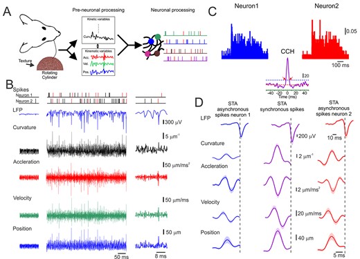
Cortical neuronal responses to tactile stimuli are composed of intermingled synchronous and asynchronized spikes. (A) Experimental paradigm. The methodology we used to investigate the vibration signals transmitted by the whiskers. The rotation of a texture-covered cylinder induced whisker vibrations. The cylinder surface was oriented so that the whisker rested on it and remained in contact during the entire whisk trajectory (left panel). We extracted whisker motion’s kinematic and kinetic characteristics (middle panel) and related them to the neuronal population activity (right panel). (B) An example of whisker motion, LFP, and spike discharge in two neurons in response to the P220 texture. The various kinematic and kinetic variables are shown in the different rows (middle panels). The left panels showed the responses when the wheel was not moving, whereas the right panel depicts a portion of the responses at a larger magnification. The spikes marked in red are synchronous. (C) Peristimulus time histogram (PSTH) and cross-correlation histogram (CCH) for the neurons in (B). The dashed horizontal line in the CCH indicates the significance level (see Methods section and Supplementary Fig. S2). The scale bar for the PSTH represents the probability of firing for a 1-ms bin. The red arrows indicate the boundaries of the time window for significant correlation. The scale bar for the CCH represents the number of spikes for a 1-ms bin. (D) STA of whisker motion and LFP for synchronous (middle panels) and asynchronous spikes (left and right panels).
Data Analysis
The significance of the differences between measured parameters was evaluated using a one-way analysis of variance (ANOVA). When significant differences were indicated in the F ratio test (P < 0.05), the Tukey method for multiple comparisons was used to determine those pairs of measured parameters that differed significantly from each other within a group of parameters (P < 0.05 or P < 0.01). The results are presented as the mean ± standard deviation (SD). Error bars in all the figures indicate the SD. Data and code available on request from the authors.
Temporal Synchronization Quantification
To quantify the temporal synchronization of the correlated firing rate which occurred within ±10 ms of the zero time lag, we used the significance ratio (SR) as a measure of synchronization. SR is the ratio of two integral values: a peak value (Peak), representing the magnitude of the spike correlation, which is computed by taking the sum of the bins in the central 20 ms of the cross-correlogram that exceeds the 95% confidence limit, and a variance value (V), representing the expected occurrence of coincident spikes, which is computed from the sum of the central 20 ms in each histogram lying between the 99% confidence limit and the mean value of the correlogram. We computed the SR as follows:
SR = Peak/V,
Each CCH was computed from the cross-correlation between each trial of two neurons and the corresponding cumulative correlogram was calculated. The SR value was computed for each CCH. For each experimental trial, we computed an equivalent pseudorandom trial (i.e., a random trial taken from 75 trials) and a shuffled trial obtained by randomly shuffling 75 trials.
To further examine the influence of the temporal pattern of spikes and the significance of temporal locking of spikes to the stimulus, we also computed an equivalent pseudorandom trial in which we shuffled the interspike intervals (ISI) within each trial. We create surrogate data that include an equal number of spikes and the same ISI distribution in each trial. This procedure shuffled spike timing and eliminated temporal locking to the SSE while keeping the number of spikes and the ISI distribution constant. An example of the CCH for the shuffled ISI is shown in Supplementary Figure S2D (lower panel). These two simulations were repeated 500 times for each CCH on each trial. This yielded 500 control SR values (pseudorandom and intertrial shuffled) for each experimental CCH. We assigned a confidence limit for statistical significance by choosing the SR values in the control distribution that were >99% of the values. An SR ratio >1 was considered significant (a graphical representation of this analysis is shown in Supplementary Fig. S2).
Calculation of the Width of the Cross-Correlogram Histogram
The CCH width was calculated as the absolute difference between the positive and negative time lag at which the CCH reached the mean + 3 SD.
Correlation Between the Cross-Correlogram SR Ratio and Width
Synchrony-Based Selection
To differentiate between synchronized and asynchronized spikes, we initially selected neurons that show significant synchronized activity in their spike trains (see above). We calculated the time window for significant correlation (the time points of the central peak in the CCH that exceeds the 3 SD threshold. Red arrows in Figure 1C). In these neurons, we searched for spikes in the two neurons that showed interneuronal ISI smaller than the chosen time window. These spikes were termed synchronized spikes, whereas spikes in the two neurons that showed interneuronal ISI larger than the chosen time window were termed asynchronized spikes.
Spike-Triggered Average
The spike-triggered average (STA) kernel was calculated by averaging the signal (whisker position, velocity acceleration, curvature) over a certain time window (kernel width = 20 ms) preceding each spike (Schwartz et al. 2006). By using different spike types as the trigger and drawing the spike-triggered ensemble from different components of the signal, we calculated STA variants, denoted STAsync and STAasync. For the STA of LFPs, we averaged the LFP signal over a 20 and 7 ms preceding and following each spike, respectively.
Detection and Quantification of SSE Underlying Spikes
To examine the relationship between SSE characteristics and the different response properties, for each spike, we detected its underlying SSE. We quantified the timing of each SSE by defining the peak value, which crossed the threshold, within 20 ms preceding each spike. The threshold used in the current study was the mean ± 3 SD (the dashed green and red horizontal lines in Fig. 4A indicate mean ± 3 SD of each trace, respectively). To define SSE timing, we detected the peak value that crossed the threshold (see Fig. 4A; red arrows for several examples of peak detection). Each SSE amplitude was calculated by measuring the peak-to-peak amplitude within ±10 ms of the largest peak. To further verify this method, we calculated the SSE-spike latency. We found that latencies were minimal at L4 [6.8 ± 0.8 ms (mean ± SD, n = 72 neurons)]. Latencies were longer at L2/3 (10.3 ± 0.9 ms, n = 82). L5 and L6 exhibited even longer latencies (9.5 ± 1.6 ms, n = 69; 13.6 ± 0.9 ms, n = 47, respectively) (Narayanan et al. 2017).
To examine whether our choice of threshold influenced our results, we measured the latency from the SSE peak to spike initiation (Fig. 4). We then estimated the SSE amplitude and spike latency (threshold = mean ± 3 SD, Fig. 4B). We found that setting different thresholds did not change the results significantly (Supplementary Fig. S10). The figure shows that the correlations between the results at the different thresholds were very high.
SSE-Dependent Firing Rates
After detecting SSE that resulted in spikes, we calculated the number of spikes following each SSE. We examined the influence of SSE amplitude on the number of spikes within the next 30-ms window for asynchronous and synchronous spikes (Fig. 3B,C).
SSE-Dependent Firing Probability
To examine the influence of SSE amplitude on discharge probability, we set a dynamic threshold from which we detected whisker vibration events. We inspected the number of spikes within the next 30-ms window for each of these events at a specified threshold. We calculated the probability of spike discharge for each threshold value by calculating the ratio of the number of spikes to the number of events. Several examples of this calculation are shown in Figure 3D and Supplementary Figure S6.
Stimulus-Dependent LFP Commencement
For each sensory-evoked spike, we identified its underlying LFP. To detect each LFP commencement, we calculated the second derivative of the LFP. This gave us the inflection point (red arrows in Fig. 5 and Supplementary Fig. S11). We calculated the time interval between the sensory-evoked commencement of LFP and the spikes from these points.
Dependence of Response Characteristics on SSE Magnitude
Results
Transformation of Tactile Inputs into Cortical Activity
To examine the transformation of the whisker interactions with surfaces into cortical neuronal discharge, we produced the whisker movements across different surfaces by covering the face of a rotating cylinder with several grades of sandpaper with different degrees of coarseness (Lottem and Azouz 2008). The cylinder face was placed orthogonally to the vibrissae so that the vibrissa rested upon it (Fig. 1A). We employed surfaces of four different grades. However, since no essential differences were found between the neuronal responses to the different textures, we lumped all the results together. The experimental strategy was to collect records of the natural movement of whiskers across surfaces and use them as a stimulus set to probe the neuronal representation of texture. In all experiments, stimuli were applied to a single whisker. An example of whisker motion across a P220 sandpaper is shown in Figure 1B. Whisker velocity and acceleration, calculated from the position trace, revealed multiple brief, high acceleration, high-velocity events that occurred during whisker motion, as well as excursions in the forces acting on the follicles. To examine the neuronal transformation of these tactile events, we recorded LFPs and spikes with multisite silicon probe electrodes from S1. Single-neuron spike trains were isolated by spike sorting (see Methods section and Supplementary Fig. S1). After separating the spike trains from different neurons, the sample consisted of 270 pairs (n = 580 neurons) recordings. For each pair, we used numerous stimuli varying in surface coarseness, distance, and speed.
Cortical Neuronal Synchrony
To examine the temporal synchronization between pairs of neurons, we calculated the cross-correlation between each spike train of paired neurons and then generated the CCH (Fig. 1C, Supplementary Fig. S2). To calculate the statistical significance of the temporal synchronization, we computed an equivalent pseudorandom spike train for each pair of neurons. Using the selection criterion of the confidence limits derived from the pseudorandom spike trains (see Methods section and Supplementary Fig. S2), the incidence and characteristics of significant response synchronizations for all neurons taken from the same tetrode for all conditions are summarized in Figure 2. We found that out of the 270 pairs, 146 pairs (54%) showed significant temporal correlations in their spike trains. Figure 2A depicts the distribution of SR values across all pairs and conditions, which indicates that a large proportion of the paired neurons had SR values above the significance level (>1). Previous studies employing cross-correlation analysis in S1 have demonstrated that correlated firing occurs on time scales of up to 20 ms (Zhang and Alloway 2004; Zhang and Alloway 2006). To determine whether our data could be categorized similarly, we computed the width at half-height of all the significant correlations in our sample. The range of temporal windows in neurons that showed a significant temporal correlation is shown in Figure 2B and ranged from 2 to 22 ms with an average of 10.9 ms. This distribution of correlation widths in our data reflects the characteristic temporal structure of the synchronous neuronal activity found in our sample. We calculated the correlations between the SR values and the width over different conditions to examine the relationship between the degree of synchronization and its temporal structure. Figure 2C shows the correlations between all pairs across all conditions and is indicative of the close relations between two characteristics of synchronous activity. Finally, we were able to establish the laminar position of 207 neurons. As indicated in Figure 2D, the incidence of neuronal synchronization was the highest in layer 4 (0.75), the lowest in the infragranular layers (0.45), and intermediate in the supragranular layers (0.49). These results suggest that neuronal synchronization at millisecond precision is a prevalent and robust feature of stimulus-evoked activity.
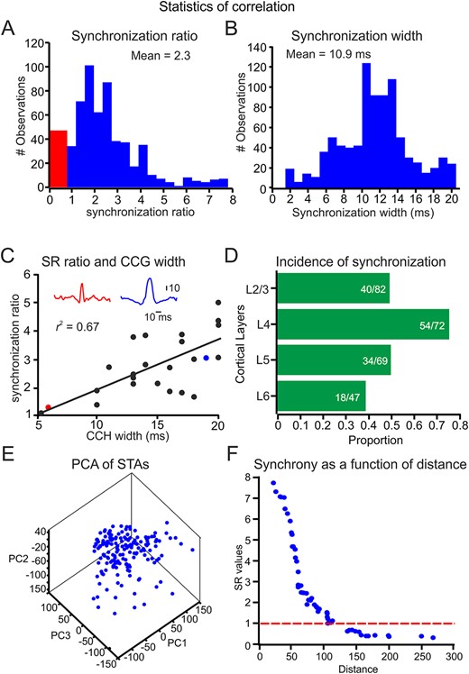
Cortical neuronal synchrony is stimulus-dependent. (A, B) Distribution of SR values. The red bins show the SR values <1 (see Methods section and Supplementary Fig. S2 for calculating this measure). (B) Distribution of the width of the central peak of all CCH. (C) The relationship between SR values and width over 24 conditions in paired neurons. In the inset, red and blue CCH are examples of the two conditions (red and blue dots in the correlation). (D) The proportion of significantly synchronized neurons from all recorded pairs in the different cortical layers. (E) A graphical representation of PCA. Each point in the 3D plot represents the three PCA components of the STA of each neuron. (F) The relationship between the Euclidean distance between paired recordings in (D) and its corresponding SR values.
Previous studies have shown that when cortical neurons are exposed to the same stimulus repetitively, a response correlation among neighboring cortical neurons is observed (Kohn and Smith 2005; Cohen and Kohn 2011). This correlation is known as the spike count correlation and may lead to spurious synchronization (Brody 1999). To examine whether cortical neurons vary in their firing rates, we calculated the z-scores relative to the mean firing rate for each trial and then plotted the normalized firing rate of the paired neurons to numerous presentations of the textures. We found that the correlation between simultaneously recorded neurons was 0.08 ± 0.02. These results suggest that barrel cortical neurons hardly covary in their firing rates.
To determine whether the stimulus drove synchronous spikes across simultaneously recorded neurons, we calculated the relationship between the similarity of the stimulus that resulted in spikes in the two neurons and the degree of synchronization. First, we calculated the STA of the stimulus for each neuron. We then used principal component analysis (PCA) to quantify these STAs. We used the first three components, which accounted for 91% of the variance. Figure 2E presents a graphical representation of this analysis. Each point in the 3D plot represents the three PCA components of the STA of each neuron. We then calculated the Euclidean distance between the different points of the paired recordings. Figure 2F shows the relationship between this distance and the SR values. These results indicate that the similarity between the STA in paired recordings could predict the synchronization between these neurons.
Further support for this proposition comes from shuffled ISI data. We create surrogate data for each session. We shuffle the ISI, thereby losing all temporal information in the response while keeping the number of spikes and ISI distribution constant (see Methods section). This analysis is shown in the lower panel of Supplementary Figure S2D,F. We found that removing the temporal information within trials eliminated almost entirely neuronal synchronization. The SR value (SR = 4.06) for these neurons was higher than the shuffled trial SR value (SR = 2.3). Together these results indicate that cortical neuronal synchrony is stimulus driven.
Rate Coding in Synchronized and Asynchronized Spikes
We next examined the role of synchronous versus asynchronous spikes in tactile transformation. All coincident spikes occurring within the significant temporal window determined by the CCH width (red arrows in Fig. 1C, lower panel) were designated synchronous and colored red; all other spikes were designated as asynchronous and colored black (Fig. 1B). To examine the robustness of our spikes partition to asynchronous and synchronized, we were able to record in some sessions from multiple neurons (n = 18; triplets and quadruplet). We then found that out of the asynchronous spikes between one pair, only 0.03 ± 0.01 were synchronized with other neurons. This small number of spikes was commonly generated at larger SSE amplitudes. As can be seen from the trace, the synchronized spikes are interspersed with nontemporally correlated spikes. An examination of the neuronal response showed that high-velocity events coincided with large magnitude in the LFP and the neuronal discharge. An expanded view of the data (Fig. 1B, right panels) revealed that more significant tactile events resulted in larger negativities in the LFP and temporally correlated spikes between the two neurons (marked in red). We calculated the STA of the synchronous and asynchronous spikes to explore how these different aspects of neuronal activity in the S1 cortex represented tactile stimuli. We posited that if a different stimulus feature drove each spike type, this should be reflected in a different STA. This is shown in Figure 1D, in which the STAs calculated from the asynchronous spikes of the neurons were smaller and had a more considerable variance. In contrast, the STAs calculated from synchronous spikes were larger and had a minor variance (see more examples of different STAs in Supplementary Fig. S3).
Inspection of the SSE amplitudes underlying all the spikes revealed a bimodal distribution (Fig. 3A, insert) in which the two types of spikes were expressed in significantly nonoverlapping peaks (Fig. 3A). Thus, the STAsync amplitudes (normalized to the z-score) were more prominent than the STAasync amplitudes in all neurons. This conclusion was also valid for all the other kinematic and kinetic variables (velocity, acceleration, curvature; Supplementary Fig. S4). These results suggest that synchronous spike activity may result from larger magnitude SSE.
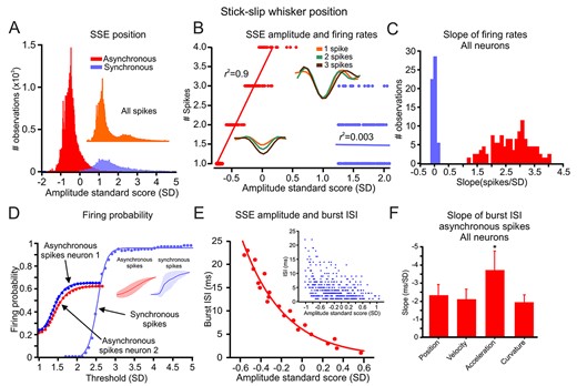
Asynchronous spikes convey the amplitude of SSE in their discharge rate, probability, and ISI. (A) Normalized distribution of SSE amplitudes that resulted in asynchronous (red) and synchronous (purple) spikes. The inset shows the distribution of all SSE that resulted in spikes. (B) The relationship between SSE amplitude and firing rates in asynchronous (red) and synchronous (purple) spikes. The lines indicate the linear regression fit. The insets show the STA for 1, 2, and 3 asynchronous and synchronous spikes. (C) Distribution of the slopes of the linear regression fit of the relationship between SSE amplitude and firing rates for all spikes in all neurons. (D) The relationship between SSE amplitude and firing probability in asynchronous (red) and synchronous (purple) spikes. A sigmoidal function could fit this relationship. The inset shows the averages for all neurons. (E) The relationship between SSE amplitude and burst ISI. The inset shows all spikes in the session, whereas the lower panels show the relationship after averaging all points within 1-ms bins. The line is the exponential decay fit of the data. (F) The mean and SD for exponential decay fit slopes for the relationship between the various SSE features and burst ISI for all asynchronous spikes in all neurons.
Given that STAs have different amplitudes depending on which spike type is used for triggering, we reasoned that these two types of activity might concurrently encode different aspects of tactile stimuli and transform these stimuli into a different facet of neuronal activity. We investigated the relationship between SSE amplitudes and the resulting neuronal discharge rates in the two groups of spikes (see Methods section). We found a linear relationship between the neuronal discharge rates and the SSE amplitude in the asynchronous spikes, but no such dependence for the synchronous spikes (Fig. 3B). Figure 3C compares the normalized slopes of the asynchronous versus synchronous spikes fit. A comparison of all neurons shows that the asynchronous spikes conveyed the SSE amplitude by their firing rates, whereas the synchronous spikes were poor at this (Fig. 3B,C; only 5% of the synchronous neurons evidenced this phenomenon). This conclusion was also valid for all the kinematic and kinetic variables [position (0.94), velocity (0.97), acceleration (0.97), curvature (0.98); the numbers in parentheses are the proportions of significant neurons manifesting this correlation; Supplementary Fig. S5].
Next, we examined the relationship between the SSE amplitudes and the discharge probability in the two types of spikes. For this analysis, an SSE was defined as any peak that crossed a defined threshold (the minimum threshold was set to 1 SD (stick vs. slip events were not distinguished). The analysis was confined to the initial 20 ms following each SSE. The net spiking probability of the asynchronous spikes increased gradually with increasing thresholds, indicating that these types of spikes can robustly convey the magnitude of SSE by their discharge probability (Fig. 3D; these relationships could be fitted by a sigmoidal function). By contrast, the synchronous spikes exhibited almost an all-or-none behavior once they reached the higher threshold (several examples of these relationships in other neurons are shown in Supplementary Fig. S6). The comparison between the two types of spikes is also depicted in the average normalized function in all neurons in Figure 3D insert. To quantify the difference between asynchronous and synchronous spikes, we plotted the distribution of slopes, the shift in the curves, and the maximal probability in all neurons. Supplementary Figure S7 confirms that the asynchronous spikes changed their discharge probability due to SSE amplitude, as indicated by the smaller slope values.
In contrast, the synchronous spikes rose sharply with the SSE amplitude. Moreover, the rightward shift in the synchronous spike curve further validates that they arose from larger amplitude SSE and resulted in a higher discharge probability (Fig. 3A, Supplementary Fig. S7). These results imply a clear distinction between asynchronous and synchronous spikes in which the former robustly convey the magnitude of smaller SSE in their discharge probability and rate. In contrast, the latter serves as an indicator of larger amplitude SSE. This conclusion was also valid for all the kinematic and kinetic variables [position (0.85, 0.97), velocity (0.83, 0.95), acceleration (0.89, 0.96), curvature (0.85, 0.95); the numbers in parentheses are the proportions of significant neurons manifesting this correlation for asynchronous and synchronized spikes, respectively; Supplementary Fig. S7].
Temporal Coding in Asynchronized and Synchronized Spikes
We reasoned that cortical neurons carry information about tactile stimuli in their temporal patterns based on many studies. To examine whether time is of the essence in conveying tactile information, we studied four aspects of temporal encoding in the neuronal spike trains: burst ISI, response latency, the relative interval between network activity and spikes, and finally, the relative spike timing between synchronous spikes. We calculated the relationship between SSE amplitude and the asynchronous spikes’ ISI. We quantified this relationship by plotting the dependence of ISI on SSE amplitude for the spikes in Figure 3A. The plots in Figure 3E show this dependence in asynchronous spikes. All asynchronous spikes are shown in the inset. We binned spike latency into 1-ms bins to plot this dependence and averaged all the SSE amplitudes for these time points. This figure shows that the ISI in the asynchronous spikes was dependent on the SSE amplitude. We then quantified this relationship by plotting the distribution of the normalized slopes in all neurons (the SSE slopes were normalized to the z score). We found that asynchronous spikes showed a significant ISI dependence on the SSE for the different kinematic and kinetic variables [position (0.74), velocity (0.78), acceleration (0.93), curvature (0.76); the numbers in parentheses are the proportions of significant neurons showing this correlation; Supplementary Fig. S8]. The larger number of neurons showing a significant correlation to SSE acceleration, and the significantly larger slope (Fig. 3F; Supplementary Fig. S9A) suggests a preferential selectivity of spike ISI for SSE acceleration.
Next, we calculated the relationship between SSE amplitude and spike latency. As previously mentioned, we divided the analysis into asynchronous and synchronous spikes. For each spike, we detected its underlying SSE. We quantified the timing of each SSE by defining the peak value, which crossed the threshold at the mean ± 3 SD (dashed red horizontal lines in Fig. 4A. The choice of different thresholds did not significantly change the results; Supplementary Fig. S10). Figure 4A shows several traces from the same asynchronous and synchronous spikes showing various latencies from their underlying SSE. The examples show that in synchronous spikes, the spike latency depended on the SSE amplitude, whereas it was not in asynchronous spikes. We quantified this relationship by plotting the dependence of the spike latency on SSE amplitude for the spikes in A. The plots in Figure 4B show this dependence in the asynchronous (left and right panels) and synchronous spikes (middle panel). All spikes in each group are shown in the insets. To make this dependence clearer, we binned the spike latency into 1-ms bins and averaged all SSE amplitudes for these time points. These figures show that the spike latency in synchronous spikes was dependent on the SSE amplitude, whereas asynchronous spikes did not manifest this dependency. We then quantified this relationship by plotting the distribution of the normalized slopes in all neurons (the SSE slopes were normalized to the z score) for synchronous and asynchronous spikes. We found that the synchronous spikes showed a significant latency dependence on the SSE position amplitude in 89% of the neurons, whereas the asynchronous spikes did not exhibit this dependence (only 12% showed a significant dependency of the asynchronous spikes; Fig. 4C,D). This conclusion was valid for all kinematic and kinetic variables [position (0.89), velocity (0.86), acceleration (0.93), curvature (0.87); Supplementary Fig. S11]. Comparison of the slopes of the relationship between the various kinetic and kinematic magnitude in synchronous spike latency did not reveal any preferential selectivity to any of these variables (Fig. 4E).
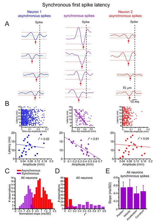
Synchronous spikes convey SSE amplitude in their spike latency. (A) Spike latency from its underlying SSE (red arrow to vertical dashed line) for synchronous (middle panels) and asynchronous spikes (left and right panels); the dashed green and red horizontal lines indicate mean ± 3 SD of each trace, respectively. (B) The relationship between SSE amplitude and spike latency in synchronous (middle panels) and asynchronous spikes (left and right panels). The upper panels show all spikes in the session, whereas the lower panels show the relationship after averaging all points within 1-ms bins. The line is the linear regression fit of the data. (C) Distribution of the normalized linear regression fit slopes for the relationships between SSE amplitude and spike latency for synchronous (purple) and asynchronous (red) spikes in all neurons. (D) Distribution of the r2 values of the linear regression fit slopes for the relationships between SSE amplitude and spike latency in all neurons. (E) The mean and SD of fit slopes for the relationship between all neurons’ different whisker motion features and synchronized spike response latency.
Next, we examined the influence of SSE amplitude on the time interval between the sensory-evoked commencement of the LFP and the spikes. To define the sensory-evoked LFP starting point, we calculated the second derivative (Fig. 5A, middle green traces; red arrows; see more examples in Supplementary Fig. S11). Once we calculated the inflection point, we calculated the LFP amplitude for asynchronous and synchronized spikes and found that synchronous spikes arose from larger LFP responses (Fig. 5C). We then calculated the influence of the SSE amplitude on the time interval between the LFP inflection point (red arrow) and the spike initiation time (dashed vertical lines). As previously mentioned, we compared synchronous with asynchronous spikes. The plots in Figure 5B show this dependence in the asynchronous (left and right panels) and synchronous spikes (middle panel; see more examples of the detection for asynchronous and synchronous spikes method in Supplementary Fig. S12. Several more examples of the dependency of LFP-first spike latency on SSE magnitude are shown in Supplementary Fig. S13). All the spikes in each group are shown in the insets. To make this dependence clearer, we binned the spike latency into 1-ms bins and averaged all the SSE amplitudes for these time bins. These figures show that the time interval between the LFP inflection point and spike initiation in the synchronous spikes was dependent on the SSE amplitude. In contrast, the asynchronous spikes did not show this dependency. We then quantified this relationship by plotting the distribution of the normalized slopes in all neurons (the SSE slopes were normalized to the z score) for synchronous and asynchronous spikes. We found that the synchronous spikes showed a significant latency dependence on SSE position amplitude in 80% of the neurons, Fig. 5D). This conclusion was valid for all kinematic and kinetic variables [position (0.8), velocity (0.88), acceleration (0.88), curvature (0.96); Supplementary Fig. S14]. The significantly larger slope (Fig. 5E; Supplementary Fig. S9B) suggests a preferential selectivity of LFP-synchronized spike latency for SSE velocity.
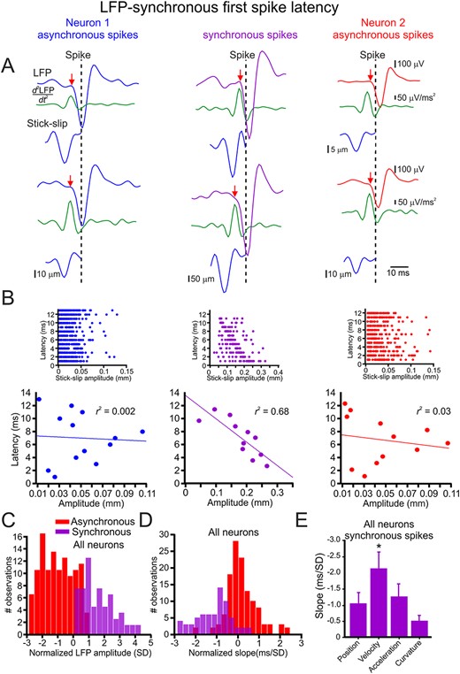
Synchronous spikes convey SSE amplitude in their LFP-spike latency. (A) Spike latency from its underlying LFP (red arrow to vertical dashed line) for synchronous (middle panels) and asynchronous spikes (left and right panels). The LFP commencement was determined by the second derivative of the LFP (green traces; see Methods section). (B) The relationship between SSE amplitude and LFP-spike latency in synchronous (middle panels) and asynchronous spikes (left and right panels). The upper panels show all spikes in the session, whereas the lower panels show the relationship after averaging all points within 1-ms bins. The line is the linear regression fit of the data. (C) Distribution of the normalized linear regression fit slopes for the relationships between SSE amplitude and LFP-spike latency for synchronous (purple) and asynchronous (red) spikes in all neurons. (D) Distribution of the r2 values of the linear regression fit slopes for the relationships between SSE amplitude and LFP-spike latency in all neurons. (E) The mean and SD of fit slopes for the relationship between the different whisker motion features and LFP-synchronized spikes latency in all neurons.
Finally, we examined the influence of the SSE amplitude on the degree of spike synchrony, that is, the interneuronal ISI. An example of this influence is shown in Figure 6A,B. The panels show that the larger SSE amplitude resulted in a smaller ISI. We then quantified this relationship in this session and found that this dependence could be fitted by an exponential decay function (Fig. 6C). Figure 6D,E shows this dependence in all neurons (90.2% of the neurons exhibited this significant dependence). While this conclusion was valid for all kinematic and kinetic variables [position (0.92), velocity (0.87), acceleration (0.88), curvature (0.96); Supplementary Fig. S15], the larger number of neurons showing a significant correlation to SSE curvature (Fig. 6F) suggests a preferential selectivity for the interneuronal ISI for SSE curvature. Moreover, the slope of this exponential decay showed a significantly steeper dependence of latency on the SSE curvature and larger r2 values (Fig. 6F, Supplementary Figs S9C and S15). Together these results strongly suggest that synchronous spikes convey different tactile characteristics via various temporal patterns.
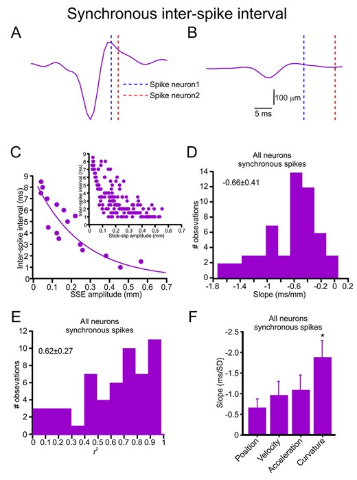
Synchronous spikes convey SSE amplitude in their interneuronal ISI. (A, B) Two examples of the dependence of synchronous spike interneuronal ISI on SSE amplitudes. (C) The relationship between SSE amplitude and interneuronal ISI. The upper panels show all spikes in the session, whereas the lower panels show the relationship after averaging all points within 1-ms bins. The line is the exponential decay fit of the data. (D) Distribution of the exponential decay fit slopes for the relationships between SSE amplitude and synchronous spike interneuronal ISI in all neurons. (E) Distribution of the r2 values of the exponential decay fits for the relationships between SSE amplitude and interneuronal ISI in all neurons. (F) The mean and SD for exponential decay fit slopes for the relationship between the various SSE features and interneuronal ISI in all synchronized neurons.
The Influence of Stimulus and Response History on Synchronized and Asynchronized Spikes
Synchronized spikes are interspersed with nontemporally correlated spikes. We compared several activity components preceding synchronous and asynchronous spikes to examine whether their occurrence was haphazard or whether the preceding activity influenced their initiation. First, we examined the relationship between the stimulus variance preceding each SSE resulting in a spike. We calculated the stimulus SD preceding each event from 5 to 200 ms and then calculated the ratio of the SD of the stimulus preceding synchronous spikes to those preceding the asynchronous spikes (Fig. 7A; Supplementary Fig. S16A). We found that this ratio was >1 (Supplementary Fig. S16A). Moreover, it emerged that 30 ms was the optimal window with the largest population of neurons showing significant correlations (Supplementary Fig. S16B). At 30 ms, the synchronous spikes were preceded by more significant stimulus variance (Fig. 7A,B).
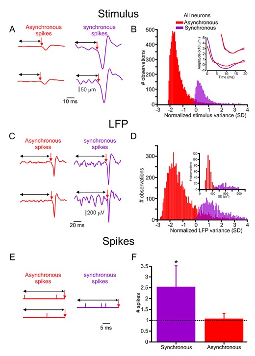
Synchronous spikes are dependent on stimulus and response history. (A) Two examples of the variance preceding SSE result in asynchronous (red traces, left) and synchronous spikes (purple traces, right). (B) Normalized stimulus variance (SD) distribution preceding SSE that resulted in asynchronous and synchronous spikes in all neurons. The inset shows the stimulus’s autocorrelation function preceding synchronous and asynchronized spikes (the smaller traces show the normalized function, which indicates that the two functions are identical in respect to their temporal structure). (C) Two examples of LFP variance preceding the LFP response that resulted in asynchronous (red traces, left) and synchronous spikes (purple traces, right). (D) Distribution of normalized LFP variance (SD) preceding the LFP response that resulted in asynchronous and synchronous spikes in all neurons. (E) The neuronal discharge precedes asynchronous (red traces, left) and synchronous spikes (purple traces, right). (F) Comparison of the number of spikes preceding asynchronous and synchronous spikes in all neurons.
Next, we examined whether the history dependence in the stimulus may influence the occurrence of synchronized spikes. We calculated the temporal correlations in the whiskers’ signal by using the autocorrelation function to study these influences. The inset in Figure 7B shows the stimulus’s autocorrelation function preceding synchronous and asynchronized spikes for the neurons in Figure 7A. We did not find any differences, except in magnitude, in these functions between asynchronous and synchronous spikes (see an example of this function in the inset of Fig. 7B). The inset shows the stimulus’s autocorrelation function preceding synchronous and asynchronized spikes (the smaller traces show the normalized function, which indicates that the two functions are identical in their temporal structure).
Third, we examined the relationship between preceding network activity and synchronous spikes. To do so, we calculated the LFP SD preceding each spike by 5–200 ms and then calculated the ratio of the SD of the LFP preceding synchronous spikes to these preceding asynchronous spikes. We found that 80 ms was the optimal window, with 90% of the neuronal population showing significant correlations (Supplementary Fig. S16D). At an 80-ms time window, the synchronous spikes were preceded by more extensive network activity (Fig. 7C,D). Finally, we examined the influence of the preceding firing rates on the synchronous spikes. To do so, we calculated the number of spikes preceding each spike by 5–200 ms and then calculated the mean number of spikes preceding the synchronous spikes and these preceding asynchronous spikes. We found that 30 ms was the optimal window for the entire neuronal population to obtain significant correlations (Supplementary Fig. S16E,F). More spikes preceded the synchronous spikes at a 30-ms time window (Fig. 7E,F). These results indicate that stimulus history, network activity, and the neurons’ activity can be future indicators of neuronal synchronization.
Discussion and Conclusions
By monitoring the kinematic and kinetic characteristics of whisker motion across textures and concurrently recording from a small population of cortical neurons, we could effectively explore the transformation of tactile inputs into cortical neuronal discharge. We employed the reverse and forward correlation methods to examine the tactile events that resulted in cortical spikes without formulating a priori assumptions about their characteristics. Our data support the idea that neurons can convey multiple tactile signals through coexisting coding strategies. We found, as others have done, that SSE resulted in increased firing rates (Diamond, von Heimendahl, and Arabzadeh 2008; Wolfe et al. 2008; Lottem and Azouz 2009; O'Connor et al. 2010; Zuo et al. 2011; Chen et al. 2015; Campagner et al. 2018); however, since we recorded from a population of neurons, we were able to monitor the degree of synchrony between adjacent neurons accurately and found that not all SSE resulted in a transient increase in firing synchrony over the background spiking. Instead, the neuronal responses to textures were composed of intermingled synchronous and asynchronized spikes. Once we separated the synchronous and asynchronous spikes, we differentiated their underlying SSE and successfully identified coexisting tactile information streams and corresponding coding strategies (Lankarany et al. 2019). Our first main result is that within a short time frame, asynchronous and synchronous spikes convey an unexpected level of stimulus detail via multiple channels, including spike rates and, most strikingly, the precise timing of spikes between and within neurons as well. These data show that cortical neurons employ coexisting stimulus encoding, in that asynchronous and synchronized spikes can simultaneously encode a large extent of tactile information. The second main result is that the different coding strategies have a differential preference for transmitting various aspects of the kinetics and kinematics of the tactile inputs. Finally, stimulus history and network activity influence the switching between the coding strategies. These findings suggest that cortical neurons may have access to a far more detailed, more dynamic description of tactile inputs than assumed.
Based on our classification of the different spike types, we found coexisting coding strategies in which several stimulus features were simultaneously represented through different spike train features. We distinguished synchronous from asynchronous spikes by a rigorous definition based on cross-correlating the spike trains of two neurons that were part of the set. Only the neurons that met the criteria (Fig. 2 and Methods section) for a significant correlation were included. Here we used the method developed by Maldonado et al. (2000)). We calculated the significant time window in the central peak of the cross-correlogram for each neuron pair and then employed this time window to search for these sporadic spikes. Thus, we showed that transient synchronization occurs in relation to external events (Riehle et al. 1997; Estebanez et al. 2012) (Fig. 2E,F). A functional interpretation of these results is expressed by the synchrony of the neuronal assembly, where jointly firing neurons form a dynamically functionally relevant subnetwork (Palm 1990; Hebb et al. 1994; Singer 1999). In the current study, the relevant functional network depends on the tactile stimulus and its history (see below). This dependency is reminiscent of several studies showing that spike synchronization changes dynamically to behavior in the primary visual cortex (Maldonado et al. 2008) and in the motor cortex (Riehle et al. 1997).
Readout Mechanisms
Access to the activity of local networks enabled us to examine whether tactile information was carried independently by each spike in each neuron or whether the information was available from the co-occurrence of spikes across two or more neighboring neurons, that is, a correlation code that depends on precise spike timing in one neuron relative to spike timing in neighboring neurons. (deCharms 1998; Sabri et al. 2016). Several studies have shown that neurons in the somatosensory cortex encode whisker-related information with a precision of a few milliseconds (Panzeri et al. 2001; Arabzadeh et al. 2006). Nevertheless, high temporal precision does not necessarily imply temporal encoding, and, in several cases, the high precision of temporal codes could be explained in terms of a rate code operating in short time windows (Borst and Theunissen 1999; Jadhav et al. 2009; Isett et al. 2018). Several decoding mechanisms that rely on determining the precise relative timing of first spikes may require the integration of “when” and “what” signals. One involves neurons that can be “tuned” to respond to a wide range of specific durations (Hooper et al. 2002). Through this mechanism, the temporal sum of the synaptic inputs of such a neuron corresponds to its firing rat (Loewenstein and Sompolinsky 2003). Within this framework, neurons can also integrate the two signals through coincidence detection mechanisms. Owing to both their intrinsic and synaptic characteristics, such neurons could be sensitive to particular temporal patterns in their inputs (e.g., the time interval between two afferent inputs), thereby converting a temporal representation of the stimulus into a firing-rate-based one (Azouz and Gray 2003; Polsky et al. 2004). The second class of mechanisms that can recognize specific temporal firing patterns may be implanted through supervised learning rules in which a neuron can distinguish between different temporal input patterns. This distinction is accomplished through the “tempotron” learning rule, which adjusts the synaptic efficacy of the different inputs. Through such learning rules, neurons can “learn” to categorize a broad range of input classes, characterized by single spikes’ latencies (Gutig and Sompolinsky 2006).
In the current study, we show that numerous neuronal codes exist within the same period that contributes to the transformation of the SSE. This coexisting coding results in multilayered coding schemes that enable spike trains to convey stimulus information through multiple complementary channels, each corresponding to a different aspect of the tactile world and its variations. Cortical neurons employ multiple types of firing rate codes at lower SSE amplitudes through asynchronous spikes. We show that cortical neurons could encode SSE magnitude using the probability and rate of asynchronous spikes (Fig. 3B–D, Supplementary Fig. S5). This coding corresponds to the commonly held view that neurons transmit information about their stimulus through their firing rate (Adrian 1926) and that spike rates correlate with the percept evoked by a stimulus (Britten et al. 1996; Romo and Salinas 2003; von Heimendahl et al. 2007; Zuo and Diamond 2019b). These findings allude to an additional coding strategy in which the clustering of spikes termed a “burst” carries specific sensory information (Reinagel et al. 1999; Kepecs and Lisman 2003; Lesica et al. 2006). Here we show that the ISIs within a burst carry information about SSE amplitude similar to what has been shown in the visual thalamus (Mease et al. 2017) (Fig. 3E,F; Supplementary Fig. S6). At larger SSE amplitudes (Fig. 3A, Supplementary Fig. S5), a tactile stimulus evokes a minority of synchronous spikes. These spikes do not transmit tactile information through firing rates or probability (Fig. 3B–D, Supplementary Fig. S5), but rather through multiple temporal coding: the first example is the latency code, in which SSE amplitude is carried by the latency of the response to the time of stimulus presentation (Fig. 4, Supplementary Fig. S10) (Gawne et al. 1996; Panzeri et al. 2001). Although this coding strategy is robust and accurate, it relies on an external temporal reference frame to define the relevant variable. However, measuring response latency relative to an external reference is not always available (Chase and Young 2007; Gollisch and Meister 2008). To avoid the need for an external reference, we measured response latency from the LFP inflection point and found a clear relationship between LFP-synchronous spike latency and SSE amplitude (Fig. 5, Supplementary Fig. S14). These results support the notion that neural codes may exploit signals intrinsically generated by the nervous system, such as population responses (Kayser et al. 2009; Knutsen and Ahissar 2009). The advantage of these coding strategies is that they can be used without detailed knowledge of external stimulus timing. Finally, another prominent example of temporal coding in the current study emerged in the interneuronal ISIs for synchronous spikes, whereby the timing of spikes to each other encoded tactile information. We found that the interval across synchronous spikes for a set of neurons is sensitive to SSE amplitude (Fig. 6, Supplementary Fig. S15). Thus, rapidly fluctuating input, resulting in presynaptic synchrony, drives more precisely timed spikes than constant or slowly fluctuating input (Bryant and Segundo 1976; Mainen and Sejnowski 1995; Nowak et al. 1997; Azouz and Gray 2008). Together, these findings show that spike timing through synchronization of neuronal assemblies is an efficient and flexible coding mechanism for sensory processing.
Stimulus Features
The different coding strategies uncovered here reflect the kinematic signatures of texture-specific whisker motion (Wolfe et al. 2008; Zuo et al. 2011). However, neurons throughout the whisker pathway, particularly in the barrel cortex, do not act as pure encoders of a single stimulus physical characteristic; instead, their preferred features tile a space defined by multiple dimensions (Maravall et al. 2007; Petersen et al. 2008; Estebanez et al. 2012; Campagner et al. 2016; Martini et al. 2017). We reasoned that a preferential selectively to any kinematic or kinetic features would be reflected in the proportion of neurons exhibiting significant correlation to any of the tactile features. Our results showed that firing rates coding do not manifest any preferential selectivity for any tactile features. However, when dealing with temporal coding, we showed that the different coding strategies did evidence a preferential selectivity for aspects of the tactile stimulus in that burst ISI showed a preferential selectivity for SSE acceleration (Fig. 3F). On the other hand, LFP-synchronous spike latency and synchronous interneuronal ISI showed a preferential selectivity for whisker velocity and curvature, respectively (Figs 5E and 6F). These results suggest that coexisting coding strategies, besides supporting the transmission of tactile information through multiple channels, also contribute to the transmission of different aspects of tactile inputs.
Response and Stimulus History
Responses to tactile stimuli are often strongly influenced by current and recent sensory experiences (Simons 1985) and intrinsic sources such as the state fluctuations of the active neuronal circuitry (Buonomano and Maass 2009; Harris and Thiele 2011). Here we show, at a single spike resolution, that the formation of synchronized activity depends not only on the stimulus presented as input to the circuit (Figs 3A and 5C) but also on the stimulus history (Fig. 7A,B) and the internal neural and network variables often denoted as the “state” of the circuit (Fig. 7C–F). Furthermore, based on the significance of the participating neurons, we found that these influences modulate the responses at different time scales (Supplementary Fig. S16):
Stimulus history was most effective at around 30 ms.
The local network showed an increase in effectiveness up to 100 ms.
The influence of preceding spikes was most influential from around 30 ms.
Note that these results refer to stimulus and network activity preceding certain aspects of sensory responses rather than the state of the network as reflected in changes in spontaneous activity preceding the external stimulus. These results thus may shed light on the constraints under which neural population codes operate (Harris and Thiele 2011).
Funding
Israel Science Foundation (950/17 to R.A.).
Notes
Conflict of Interest: None declared.