


Abstract
Feedback-related negativity (FRN) is believed to encode reward prediction error (RPE), a term describing whether the outcome is better or worse than expected. However, some studies suggest that it may reflect unsigned prediction error (UPE) instead. Some disagreement remains as to whether FRN is sensitive to the interaction of outcome valence and prediction error (PE) or merely responsive to the absolute size of PE. Moreover, few studies have compared FRN in appetitive and aversive domains to clarify the valence effect or examine PE’s quantitative modulation. To investigate the impact of valence and parametrical PE on FRN, we varied the prediction and feedback magnitudes within a probabilistic learning task in valence (gain and loss domains, Experiment 1) and non-valence contexts (pure digits, Experiment 2). Experiment 3 was identical to Experiment 1 except that some blocks emphasized outcome valence, while others highlighted predictive accuracy. Experiments 1 and 2 revealed a UPE encoder; Experiment 3 found an RPE encoder when valence was emphasized and a UPE encoder when predictive accuracy was highlighted. In this investigation, we demonstrate that FRN is sensitive to outcome valence and expectancy violation, exhibiting a preferential response depending on the dimension that is emphasized.
Humans learn about environmental regularities by forming associations among stimuli, responses, and outcomes. Hence, understanding the neural mechanisms that underlie this basic learning process has become an integral undertaking in neuroscience. In this process, prediction error (PE: the difference between outcome and expectancy) is essential (Sutton and Barto 1998). A neural manifestation of PE is a scalp-recorded electrophysiological component known as feedback-related negativity (FRN), which is defined as a negative-going difference wave (worse-than-expected events minus better-than-expected events) peaking at approximately 250 ms post-feedback (Miltner et al. 1997; Nieuwenhuis et al. 2004a). Numerous studies demonstrate that the feedback-related potentials to unfavorable events is more negative than that to favorable events, and their difference is significantly larger when outcomes are unexpected (Holroyd et al. 2003; Cohen et al. 2007; Hajcak et al. 2007; Warren and Holroyd 2012). Accordingly, reinforcement learning (RL) theory, a dominant model for FRN, posits that this event-related potential (ERP) component reflects reward prediction error (RPE), which is a teaching signal indicating whether the actual outcome is better (positive prediction error, +PE) or worse (negative prediction error, –PE) than expected (Gehring and Willoughby 2002; Holroyd and Coles 2002; Hajcak et al. 2006; Caplin and Dean 2008; Walsh and Anderson 2012; Sambrook and Goslin 2015), and presumes that FRN encodes the interaction between outcome valence and its deviation from expectancy.
However, Talmi et al. (2013) investigated feedback-related potentials to monetary reward and pain shock and found that the omission of both reward (–PE) and pain (+PE) induced more negative waves than their respective deliveries. Similarly, Huang and Yu (2014) revealed more negative waves for reward and loss omission than for delivery. These results challenge the valence evaluation of RL–RPE. Others suggest that FRN encodes an expectancy violation but not outcome valence, leading to a new account for FRN, that is, unsigned prediction error (UPE) theory (Luu and Pederson 2004; Oliveira et al. 2007; Ferdinand et al. 2012; Hauser et al. 2014). Notably, FRN is an assumed subcomponent of the frontal control-related N200 (Folstein and Van Petten 2008), which is sensitive to cognitive conflict and unexpected outcomes and shares a striking resemblance to FRN in terms of time range, polarity, and topography (Holroyd 2004). The reported UPE encoder during FRN interval may be a special case of N200 when the effect of reward is underemphasized or obscured by the effect of reward-independent PE (expectancy violation). In fact, FRN has been thought to respond selectively to multiple factors (e.g., outcome magnitude, likelihood, valence, or their interaction; Sambrook and Goslin 2015) depending on the factor that is emphasized (Nieuwenhuis et al. 2004b). Therefore, the inconsistent interpretations of FRN may be due to the heterogeneity of highlighted dimensions.
Accordingly, we hypothesized that the reward-independent effect of expectancy violation would induce an N200-like component (UPE); however, when highlighted, the reward effect would interact with expectedness and produce a difference wave as per RL theory (namely, RPE). To investigate these hypotheses, the present study conducted three ERP experiments across which the two dimensions were emphasized differently. In Experiment 1, both outcome valence and expectancy violation were included in the feedback, but neither of them was intentionally emphasized to be consistent with related studies, which allowed for a comparison with current results. In Experiment 2, to examine whether the UPE encoder is a special case of N200 that reflects the effect of reward-independent PE, purely digital forms of feedback were presented. This digital task was essential to test the mere effect of expectancy violation where the reward effect was removed. Finally, in Experiment 3, the parameters were identical to those of Experiment 1 except that outcome valence was emphasized in some blocks while predictive accuracy was emphasized in others, thereby allowing for our predictions to be directly and strictly examined.
Interestingly, although the RL–RPE theory asserts that the response patterns of feedback-related potentials are opposite in appetitive and aversive domains and some studies have documented the feedback evaluation’s sensitivity to outcome domains (Metereau and Dreher 2013; Yu and Zhang 2014; Sambrook and Goslin 2016), the RPE encoder is often revealed only in the appetitive domain (reward vs. no reward) or in mixed domains (win vs. loss) (Gehring and Willoughby 2002; Hauser et al. 2014; Silvetti et al. 2014; Mushtaq et al. 2016). To circumvent the issue concerning outcome domains, Experiments 1 and 3 investigated feedback-related potentials to the gain and loss domains, respectively. By comparing actual outcomes with expected outcomes, four types of outcome emerged: higher- or lower-than-expected gain and higher- or lower-than-expected loss. RPE would predict that higher-than-expected gain and lower-than-expected loss are favorable outcomes and should therefore elicit more positive waves than unfavorable outcomes. By contrast, UPE would predict similar response patterns between the appetitive and aversive domains.
The statistical tests based on grand average ERP waveforms often conceal intertrial and intersubject variability, which are unable to describe dynamic change. Unlike trial-average analysis, trial-by-trial correlation analysis can reveal the dynamic modulation of behavioral performance on electroencephalogram (EEG) activity (Philiastides et al. 2010). Importantly, the RPE and UPE accounts will provide clear and different predictions for this dynamic modulation. As illustrated in Fig. 1A, according to RPE, the feedback-related potentials are more negative with the increasing degree to which outcomes are worse than expected, whereas in terms of UPE, they are more negative with the increasing deviation of expectation regardless of the outcome valence. Thus, a single-trial correlation (i.e., continuous FRN–PE correlation) analysis can allow us to clearly examine these distinct predictions for RPE and UPE. Despite single-trial regression analysis demonstrating that feedback-related ERP components could predict model-derived PEs (Philiastides et al. 2010), it remained unclear as to whether relations to +PEs and –PEs were monotonic positive/negative or symmetric. Meanwhile, other studies using single-trial correlation analysis did not measure prediction and thus roughly calculated the PE value as the difference between actual outcomes and the median of those outcomes (Sambrook and Goslin 2014) or simply divided the larger-half feedback as +PE trials and the smaller half as –PE trials (for gain, and the loss was the reverse) (Sambrook and Goslin 2016). Therefore, the exact relations between feedback-related potentials and PEs could not be determined. In the present investigation, we explicitly measured the participants’ predictions via a task in which the participants entered their expected values on a scale of 0 to 20 and delivered feedback within the same scale in each trial, through which we could calculate continuous PEs for each trial and subsequently test the quantitative modulation of PE value on FRN. Specifically, we ran a single-trial Pearson correlation between PEs and ERP data at each sample point for each trial, thereby generating correlation waveforms analogous to conventional ERPs. Furthermore, we performed a temporospatial principal components analysis (PCA) on correlation waveforms to separate the potential overlapping components.
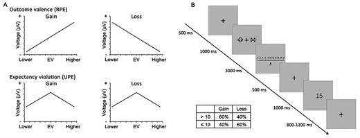
(A) Schematic responses of feedback-related potentials with respect to RPE and UPE encoders. The upper panel represents RPE, which proposes that the feedback-related potentials should be more negative for worse-than-expected outcomes. The lower panel represents UPE, which argues that the feedback-related potentials may become more negative with the increasing deviation of expectation regardless of the outcome valence. “EV” denotes the expected value. The right side of the horizontal axis represents the higher-than-expected feedback; the left-side signals the lower-than-expected feedback. (B) Schematic of experimental procedure. The time course of one trial is designated; the feedback contingencies associated with high- and low-value shapes are illustrated.
Moreover, in the current study, each trial had a non-null feedback (i.e., always delivery and no omission). Although both reward and punishment are believed to be motivational salient events (Sambrook and Goslin 2014; Hird et al. 2018), which renders their delivery more salient than omission (Esber and Haselgrove 2011), thus making salience an inevitable confounding variable, previous studies did not control its influence because they usually used all-or-nothing outcomes where the delivered condition had a higher salience than the omission condition (Talmi et al. 2013; Gu et al. 2016). However, in the present investigation, salience difference that is due to delivery and omission could be fully excluded by consistently delivering a number from 0 to 20 as feedback.
Experiment 1
Materials and Methods
Participants
Thirty participants were recruited from Southwest University (China) for monetary payment. All participants were right-handed; had no psychiatric, neurological, or medical illnesses; and reported normal or corrected-to-normal vision. Seven participants were disqualified: one for being too young (17 years old), three for having incomplete recordings, and three for producing bad EEG signals (excessively large blink artifacts). The remaining 23 participants (10 males, 19.74 ± 1.54 years old) were deemed valid for final analysis. The participants signed written consent forms upon their arrival. The study followed the guidelines of the Helsinki Declaration and was approved by the Human Ethics Committee of Southwest University.
Stimuli and Procedure
This experiment adopted a probabilistic learning task (see Fig. 1B) and was programmed using E-Prime 2.0 (Psychology Software Tools, Inc. Pittsburgh, PA) with a gray background. We manipulated financial incentives to compare the feedback-related potentials in the appetitive (gain) domain and the aversive (loss) domain. Given the context-dependent nature of outcome evaluation (Holroyd et al. 2004; Nieuwenhuis et al. 2005b), the gain and loss domains were divided into separate blocks. Prior to each block, we informed the participants via written instruction that the forthcoming block was a gain or a loss.
In the gain blocks, each trial started with a 500 ms fixation cross, followed by the display of two geometric shapes at the right and left of the fixation for 1000 ms (the left and right positions were counterbalanced across trials). Participants were told beforehand that one of two shapes was, on average, associated with a slightly higher gain than the other and that they could press “Q” for the left one or “P” for the right one. After their selection, the shapes disappeared, and a point scale (0–20) was presented at the center for 3000 ms. The point represented the money they might win, which was linked to their selected shape, and one point was worth one renminbi (RMB, approximately $0.15). Here they needed to predict the upcoming monetary gain by moving the bar on the scale to their expected value. Pressing “Q” could slide the bar to the left and “P” to the right. After participants entered their expected value, another fixation cross was presented for 500 ms. At the offset of this display, a value between 0 and 20 was delivered as feedback (1000 ms), representing the money they actually obtained. Finally, a gray screen with a variable duration (800–1200 ms) was shown as an intertrial interval.
The loss blocks followed a similar procedure as that of the gain ones; however, participants were told that one of two shapes was associated with a slightly lower loss than the other. Accordingly, the point scale denoted the money they might lose in relation to the selected shape, and they needed to predict the upcoming monetary loss by moving the bar to their expected value. The final delivered feedback represented the money they lost in actuality.
In this experiment, given the opposite valence of gain and loss, the higher-than-expected gain and lower-than-expected loss were regarded as +PE trials while the lower-than-expected gain and higher-than-expected loss were regarded as –PE trials. These aspects also denoted the degree of expectancy violation (absolute PE; cf. instantiated examples in Table 1).
Proposed PEs with respect to RPE and UPE accounts using instantiated examples
| Domain | Prediction | Feedback | RPE | UPE |
|---|---|---|---|---|
| Gain | 10 | 15 | +5 | 5 |
| 10 | 5 | −5 | 5 | |
| Loss | 10 | 15 | −5 | 5 |
| 10 | 5 | +5 | 5 |
| Domain | Prediction | Feedback | RPE | UPE |
|---|---|---|---|---|
| Gain | 10 | 15 | +5 | 5 |
| 10 | 5 | −5 | 5 | |
| Loss | 10 | 15 | −5 | 5 |
| 10 | 5 | +5 | 5 |
The participants completed 10 practice trials before the main procedure. The main experiment included four blocks each for the gain and loss domains (40 trials per block, 320 total trials), with a self-paced break between blocks. Half the participants completed four gain blocks first and then four loss blocks; this sequence was reversed for the other half. We included two geometric shapes for each block, resulting in a total of 16 unique shapes. At the end of each block, the participants were asked which shape corresponded to a slightly higher gain (in the gain blocks) or a lower loss (in the loss blocks). To motivate their engagement, we told them that we would add or subtract the percentage of cumulative gain and loss from their reward depending on their performance (correct discrimination of two shapes). The entire experiment lasted approximately 50 minutes.
The overall feedback (see Fig. 1B) was slightly higher in the gain blocks (the feedback was below 10 points in 40% of the trials and above 10 points in 60% of them) yet slightly lower in the loss blocks (the feedback was below 10 points in 60% of the trials and above 10 points in 40% of them). Notably, the participants were uninformed of these probabilities. As in Sambrook and Goslin (2016)‘s study, all the feedback was pseudo-randomly predetermined and was thus unrelated to the participants’ selections yet unknown to them. Although this would result in no fixed association between shapes and feedback, with a subtle proportion difference between higher (>10) and lower (≤10) feedback (40% vs. 60%), it could largely increase the task’s difficulty. Because the actual feedback was unrelated to the selected shape, the correctness of participants’ discrimination between two shapes at the end of each block was pseudo-randomly predetermined but had to be unobtrusive. Thus, we asked the participants how they felt about the task at the end of each block to ensure whether they had discovered the fictitious associations. After the experiment, each participant earned 50 RMB for their participation in addition to a randomly determined bonus of 0–10 RMB.
EEG recording and preprocessing
We conducted the experiment in a dimly lit and soundproof room. EEG data were recorded using a 64-channel Brain Products system (Brain Products GmbH, Germany; passband: 0.01–100 Hz, sampling rate: 500 Hz) with tin electrodes mounted on a standard elastic cap based on the international 10–20 system. All signals were referenced to the fronto-central (FCz) site but were re-referenced offline to the average of the left and right mastoids; subsequently, the FCz signal was recovered. Horizontal eye movement was monitored by an electrode on the outer canthus of the right eye, and vertical eye movement was monitored using an electrode below the left eye. All electrode impedances were kept below 10 kΩ. We filtered the data offline with a bandpass filter of 0.01–30 Hz and then performed an independent component analysis (ICA) for each participant to identify and discard eyeblink-associated components. Trials that were contaminated with artifacts of amplifier clipping and bursts of electromyography (EMG) activity with peak-to-peak deflections exceeding ±80 μV were rejected before averaging.
Behavioral Analysis
Each trial recorded the participants’ choice of shape and corresponding prediction as well as the feedback. First, we analyzed their predictions throughout one block to examine how they filtered their predictions to discriminate high-value shape from low-value one. Because there was no prior knowledge regarding the association between shapes and feedback to draw from, we assumed that no difference may exist between the predictions for two shapes at the beginning of one block but that participants, proceeding with the task, would develop a preference for a good shape (higher gain or lower loss) and successfully discriminate the two shapes. Specifically, to illustrate the progressive development of their predictions, these predictions were divided into several phases for the two shapes (four trials per phase), which were then compared between two shapes at each phase using a paired-samples t-test. Although our feedback was pseudo-random and the same for all participants, we suggested that based on individual shape selection, one shape might be incidentally superior over another within one block. Notably, no fixed association existed between shapes and feedback; thus, a high- or low-value shape was defined individually based on their ratings, which were taken at the end of each block. In other words, the shape that participants reported as corresponding to higher values was labeled as “high value” and the one that they believed to be related with lower values was labeled as “low value.”
Trial-wise PE was then calculated by subtracting the expected value from the actual value. Furthermore, to verify whether the PEs were really employed as learning signals to facilitate behavioral adaptation, that is, the prediction adjustment for a specific shape should scale with the PE value from the previous encounter of that shape, we calculated the correlation between the prediction adjustment size (predictionN − predictionN − 1) and the PE of trial N − 1 for high- and low-value shapes, respectively.
ERP Analysis
EEG data were analyzed within BrainVision Analyzer 2.0 (Brain Products GmbH, Germany). For the present purpose, we analyzed ERPs time-locked to 200 ms before the onset of feedback to 600 ms afterward, which was then baseline-corrected using the epoch −200–0 ms. According to the prediction–feedback difference, six types of trials were created: expected gain (zero PE), higher-than-expected gain (H-gain: +PE), lower-than-expected gain (L-gain: –PE), expected loss (zero PE), higher-than-expected loss (H-loss: –PE), and lower-than-expected loss (L-loss: +PE). After excluding trials related with EEG artifacts, 95.22% of the trials remained for the gain domain and 94.84% remained for the loss domain. The specific number of valid trials for each condition is listed in Table S1 (see supplementary materials). In addition, all malfunctioning electrodes were substituted with an average of surrounding electrodes.
The ERPs of the aforementioned trials were created separately for gain and loss domains. Subsequently, a repeated-measure one-way ANOVA was conducted on these ERPs for each domain at the FCz site within a time window of 240–340 ms following the suggestion of a meta-analysis (Sambrook and Goslin 2015). Consistent with most studies that assessed FRN using the difference wave approach by subtracting the waveform of +PEs from –PEs (valence effect) (Holroyd and Coles 2002; Talmi et al. 2013; Sambrook and Goslin 2015), we subtracted the waveform of H-gain (+PE) from that of L-gain (–PE) and the waveform of L-loss (+PE) from that of H-loss (–PE). In the loss domain, because a “reverse” positivity was present when the result was being inspected, we conversely subtracted the waveform of H-loss (–PE) from that of L-loss (+PE). Same as Sambrook and Goslin (2014), we also computed a difference wave by subtracting the waveform of +PEs from that of –PEs across the domains.
Correlation Analysis
In the current experiment, for each trial, the continuous PE value could be calculated by subtracting the expected value from the actual value, which was then correlated with trial-wise ERP data through a single-trial Pearson correlation analysis to clarify their correspondence. This procedure enabled us to compare the parametric modulations of ±PEs in the gain and loss domains.
Following the approach of Sambrook and Goslin (2014, 2016), we calculated the Pearson correlation coefficient between the PE value and feedback-related potentials at each sample point for each trial. Because the time window analyzed in this experiment was −200–600 ms (sampling rate: 500 Hz), there were 400 sample points, and the data point used to calculate the correlation coefficient at each sample point corresponded to an individual trial. Thus, this correlation was calculated between trial-wise voltage and PE for each sample point, each electrode, and each participant. Because voltage varied over time, these correlation coefficients would also vary over time (different correlation coefficients calculated at 400 sample points). These r-values were then plotted against time to produce a correlation waveform similar to conventional ERPs but represented PE encoding strength (the correlation between feedback-related potentials and PEs). In this plot, when the waveform was at zero (baseline), it suggested that PE had no effect on the feedback-related potentials; when the waveform deviated from the baseline, a positive or negative correlation with PE was observed. Because our correlation coefficients were derived from trial-wise voltage and PE with substantial intertrial and intersubject variabilities, they were expected to be relatively small. A one-sample t-test was conducted on the correlation waveform’s peak amplitude across subjects within a 240–340-ms time window (Sambrook and Goslin 2014, 2016). Notably, rather than directly comparing the peak amplitude of +PE with –PE (i.e., paired-samples t-test), we examined the presence or absence of correlation (one-sample t-test) because the relative sensitivity to +PE and –PE was meaningless in differentiating the RPE or UPE encoder (Sambrook and Goslin 2016).
Principal components analysis
Principal components analysis (PCA) aims to dissociate the potential overlapping components from a simple averaged waveform within the same temporal interval and spatial distribution. Here, the PCA approach was conducted on the preceding correlation waveforms using the open source MATLAB program, the ERP PCA Toolkit (version 2.61). A two-step sequential PCA was performed following published guidelines (Dien et al. 2005, 2007; Dien 2010a) and studies (Foti et al. 2011; Sambrook and Goslin 2016); this approach is said to produce modestly superior results over other methods (Dien 2010b). The first step was a temporal promax rotation, and the second was a spatial infomax rotation (ICA). To guarantee that the components identified in the gain domain were exactly the same as those in the loss domain, we employed this temporospatial PCA method across the two domains.
First, a temporal PCA was conducted to capture the time variance using each time point as variables, and the combinations of participants, recording sites, and conditions (higher- or lower-than-expected outcomes) were taken as observations. To determine the number of factors to retain, we conducted a parallel test by comparing the scree plot of our dataset with the null dataset (Horn 1965). This suggested 13 factors for retention, which were then subjected to a promax rotation. The resulting factor score represented that factor’s captured variance. Second, we entered these temporal factors into a spatial PCA. In this step, the recording site was taken as a variable, and the combinations of participants, conditions, and temporal factors were taken as observations. Based on the screen plot, 3 factors were suggested for retention, yielding a total of 39 temporospatial factors, which were all subjected to an infomax rotation. Finally, these factors were reconstructed into waveforms by multiplying the produced factor pattern matrix with its standard deviation. Because the correlation waveforms that underwent this PCA denoted PE encoding strength, each factor’s PE sensitivity could be evaluated by testing its peak amplitude using the one-sample t-test as in the preceding correlation analysis.
Results
Behavioral Results
All feedback was pseudo-randomly predetermined and was thus unrelated to the participants’ selections. After each block, most participants reported that the task was difficult, and none had recognized that their choice of shape could not change the outcomes.
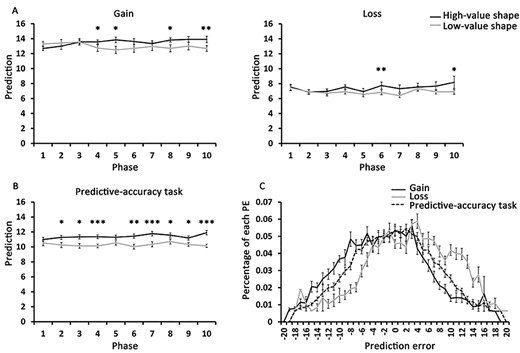
The participants’ predictions were illustrated at 10 phases throughout the block for two shapes separately. As displayed in Fig. 2A, in both domains, the high-value shape’s expected value did not differ from that of the low-value shape at the start of one block, but as the task proceeded, its value was significantly higher than that of the low-value shape, suggesting that participants displayed progressive discrimination between high- and low-value shapes as they proceeded with the task.
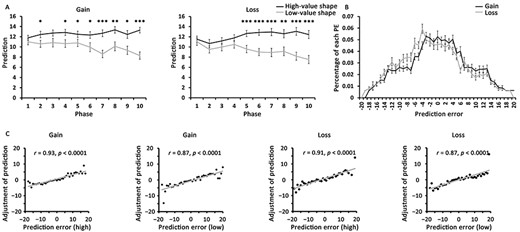
Behavioral results of Experiment 1. (A) Development of participants’ expected values for high- and low-value shapes throughout the block. Their predictions were divided into 10 phases (four trials per phase) on each block. In both domains, the participants progressively discriminated between the high- and low-value shapes as the task continued. (B) describes the PE distribution. It shows approximately normal distributions. (C) Correlations between the adjustment size of prediction (predictionN − predictionN − 1) and the PE of trial N − 1 for high- and low-value shapes. The scatterplots illustrate the across-subjects correlations. The error bar denotes standard errors. * denotes P < 0.05, ** denotes P < 0.01, and *** denotes P < 0.001.
The difference computation between expected and actual values generated continuous PEs ranging from −20 to 20, manifesting approximately normal distributions in both the gain (skewness = −0.05, kurtosis = −0.64) and loss domains (skewness = 0.16, kurtosis = −0.63) (Fig. 2B). Furthermore, Pearson correlations between the adjustment size of prediction (predictionN − predictionN − 1) and the PE of trial N − 1 were significant for both high- (across subjects: r = 0.93, P < 0.0001; mean r = 0.62) and low-value shapes (across subjects: r = 0.87, P < 0.0001; mean r = 0.63) in the gain domain as well as for high- (across subjects: r = 0.91, P < 0.0001; mean r = 0.62) and low-value shapes (across subjects: r = 0.87, P < 0.0001; mean r = 0.66) in the loss domain (Fig. 2C). These results confirmed that our participants were actually engaged in learning the shape–feedback associations and adjusted their predictions based on experienced PE values.
ERP Results
The ERPs showed negative-going waves in the gain domain (Fig. 3A) for all three conditions (F2 = 15.76, P < 0.0001) in the 240–340-ms time window at the FCz site. In particular, the waveform of expected gain (zero PE; mean = 10.40 μV) was significantly more positive than that of H-gain (mean = 7.27 μV; t22 = 3.26, P = 0.004) and L-gain (mean = 6.29 μV; t22 = 5.33, P < 0.0001), and H-gain was more positive than L-gain with a marginal significance (t22 = 2.00, P = 0.058). Similarly, three negative-going waves were observed in the loss domain (F2 = 3.49, P = 0.059) (Fig. 3B); the waveform of expected loss (zero PE; mean = 7.48 μV) did not differ from that of H-loss (mean = 6.41 μV; t22 = 1.37, P = 0.186) but was significantly more positive than that of L-loss (mean = 5.49 μV; t22 = 2.13, P = 0.045); and H-loss was more positive than L-loss with a marginal significance (t22 = 1.97, P = 0.061). Therefore, these ERP results did not align with RL–RPE theory, which states that the response patterns to +PEs and –PEs in the gain domain must be opposite to those in the loss domain.
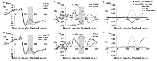
Event-related potential (ERP) results of Experiment 1 at the fronto-central (FCz) site. The ERPs are plotted separately for gain (A) and loss (B) domains. In both domains, there were apparent negative-going waves within the 240–340-ms time window (shaded area). The correlation waveforms for gain (C) and loss domains (D). We calculated the Pearson correlation coefficient between the trial-wise PE and waveform and generated correlation waveforms that represented PE encoding strength. The principal components analysis (PCA) factors extracted from the preceding correlation waveforms for gain (E) and loss domains (F). All factors are denoted in unit r against time and plotted separately for higher- and lower-than-expected feedback.
Subtracting the waveform of +PEs from that of –PEs revealed a marginally significant negativity in the gain domain (t22 = 2.00, P = 0.058; Fig. S1A). In the loss domain, a “reverse” positivity was found; however, subtracting the waveform of the H-loss (–PE) from that of the L-loss (+PE) resulted in a marginally significant negativity (t22 = 1.97, P = 0.061; Fig. S1B). Furthermore, the difference wave assessed by subtracting the waveform of +PEs from that of −PEs across the domains was not significant (t22 = −0.08, P = 0.936). Corresponding scalp topographies for the ERPs and difference waves were illustrated in supplemental materials.
Correlation Results
The single-trial Pearson correlation between the trial-wise PE and waveform reflects the degree to which the feedback-related potentials encode PEs. As displayed in Fig. 3C and D, a significant negative correlation was found on the peak amplitude of the correlation waveform for H-gain (r = −0.08 ± 0.14; t22 = −2.51, P = 0.02) and a significant positive correlation for L-gain (r = 0.07 ± 0.13; t22 = 2.66, P = 0.014). In the loss domain, no significant correlation was found for H-loss (r = −0.02 ± 0.14; t22 = −0.66, P = 0.515), but a significant positive correlation was observed for L-loss (r = 0.14 ± 0.09; t22 = 7.41, P < 0.0001). The negative correlation for H-gain indicated that the increasing PE (increasing absolute PE) was associated with decreasing ERP waveform (more negative); while the positive correlation for L-gain and L-loss indicated that the decreasing PE (increasing absolute PE) was associated with decreasing ERP waveform (more negative). Thus, a UPE encoder was supported in the gain domain where the feedback-related potentials were more negative with increasing deviation of expectation (increasing absolute PE) regardless of the outcome valence (cf. Fig. 1A). In the loss domain, although no significant correlation was observed for H-loss, the positive correlation for L-loss was inconsistent with RL-RPE theory that suggests a negative correlation for L-loss.
PCA Components
The two-step PCA across the domains resulted in 39 temporospatial factors. The first three factors were selected for further statistical analysis because they accounted for the most data variance. Notably, the spatial PCA, based on the proceeding temporal PCA, would result in temporospatial factors that reflected the variance of both temporal and spatial PCA. These factors are listed in Table 2 and plotted separately for the gain (Fig. 3E) and loss (Fig. 3F) domains.
PCA factors extracted from the preceding correlation waveforms for statistical analysis in Experiment 1
| Proposed component | Factor | Temporal peak (ms) | Spatial peak | Variance explained (%) |
|---|---|---|---|---|
| Slow wave | TF1/SF1 | 544 | CP1 | 7.97 |
| FRN | TF2/SF1 | 298 | FC3 | 6.35 |
| P3 | TF3/SF1 | 374 | FC3 | 5.47 |
| Proposed component | Factor | Temporal peak (ms) | Spatial peak | Variance explained (%) |
|---|---|---|---|---|
| Slow wave | TF1/SF1 | 544 | CP1 | 7.97 |
| FRN | TF2/SF1 | 298 | FC3 | 6.35 |
| P3 | TF3/SF1 | 374 | FC3 | 5.47 |
First, factor TF2/SF1 resembled FRN’s temporal and spatial features. The one-sample t-test on this factor’s peak amplitude revealed a marginally significant negative correlation for H-gain (t22 = −2.03, P = 0.054) but a significant positive correlation for L-gain (t22 = 3.17, P = 0.004). In the loss domain, there was no significant correlation for H-loss (t22 = 0.39, P = 0.698); however, the correlation was significantly positive for L-loss (t22 = 7.99, P < 0.0001). This factor’s response profile was similar to those of the preceding correlation waveforms.
The temporal and spatial features of factor TF3/SF1 seemed to resemble the P3 component. The one-sample t-test on this factor’s peak amplitude revealed a nonsignificant correlation for H-gain (t22 = −1.24, P = 0.227) but a marginally significantly positive correlation for L-gain (t22 = 1.96, P = 0.063). In the loss domain, it displayed a marginally significant negative correlation for H-loss (t22 = −1.78, P = 0.089) but a significant positive correlation for L-loss (t22 = 4.17, P < 0.0001).
The third factor, TF1/SF1, showed a profile similar to that of slow wave, displaying a significant positive correlation for H-gain (t22 = 2.20, P = 0.038) but a significant negative correlation for L-gain (t22 = −2.90, P = 0.008). In the loss domain, it manifested a significant positive correlation for H-loss (t22 = 5.20, P < 0.0001) but a nonsignificant correlation for L-loss (t22 = −1.54, P = 0.139).
Discussion of Experiment 1
In this experiment, the participants were instructed to learn the associations between feedback and shapes. Nevertheless, all feedbacks were pseudo-randomly delivered yet unknown to the participants; furthermore, the proportion difference between higher (>10) and lower (≤10) feedback was minute (40% vs. 60%), which largely increased the difficulty of discriminating high- and low-value shapes. As a result, all the participants reported that the task was relatively difficult after each block, and none had recognized the fictitious associations. Nonetheless, the participants progressively discriminated between the two shapes as the task proceeded (Fig. 2A), implying that they were engaged in association learning as the experimental design intended. This result is consistent with that of one study where some icons remained more profitable than others despite participants being explicitly told that the outcomes were utterly random (Sambrook and Goslin 2014).
Fig. 3A and B show that negative-going ERP waves were observed in all conditions, in which the waveform of lower-than-expected outcomes was more negative than that of higher-than-expected outcomes in both domains, producing marginally significant negativities when subtracting the waveform of higher-than-expected outcomes from that of lower-than-expected outcomes. Importantly, the single-trial Pearson correlation, which aimed to illustrate the dynamic modulation of PEs on feedback-related potentials, produced a negative correlation for higher-than-expected gain but positive correlations for lower-than-expected gain and loss (Fig. 3C and D). The PCA procedure showed similar results (Fig. 3E and F). These results were inconsistent with RL–RPE theory, which posits that the feedback-related potentials of –PEs (L-gain, H-loss) must be more negative than those of +PEs (H-gain, L-loss) and exhibit more negative waves with increasing degree to which outcomes are worse than expected (cf. Fig. 1A). Conversely, a UPE encoder was supported here, particularly because of the negative correlation for H-gain and the positive correlation for L-gain. In the loss domain, although no significant correlation was observed for H-loss, the positive correlation for L-loss was inconsistent with RL–RPE theory (suggesting a negative correlation for L-loss).
Experiment 2
In Experiment 1, the high task difficulty might draw participants’ main attention to their own prediction accuracy, thereby resulting in less attention to outcome valence. To examine this, we conducted Experiment 2 in which the task was the same as that in Experiment 1 except pure digital feedback was used. In this case, the feedback simply indicated prediction accuracy. We predicted that if the absence of RPE encoder in Experiment 1 was due to the obscureness of valence effect, then a similar result pattern would be found in Experiment 2, where the reward effect was removed. Finally, because the random feedback largely increased task difficulty and might obstruct the real learning of shape–feedback relations, these associations were fixed in Experiment 2 instead; that is, the high-number shape was truly related with higher feedback and the low-number shape with lower feedback.
Materials and Methods
Participants
Thirty-five participants from Southwest University (China) volunteered for this experiment for monetary compensation. All the participants were right-handed and had normal or corrected-to-normal vision. None reported any psychiatric, neurological, or medical illness. Seven participants were removed: two for misunderstanding the task rule and another five for having excessively large artifacts on EEG signals. The remaining 28 participants (15 males, 19.71 ± 1.67 years old) underwent the final statistical test. Each participant provided written consent upon their arrival. The study was approved by the Human Ethics Committee of Southwest University and complied with the Helsinki Declaration guidelines.
Stimuli and Procedure
The experimental procedure was the same as in Experiment 1. Experiment 2 included six blocks (40 trials per block, 240 trials total); each block included two unique shapes, resulting in a total of 12 shapes. To motivate the participants’ task involvement, we informed them beforehand that correct discrimination could earn them an extra 2 RMB. After the experiment, the participants were paid 50 RMB and a performance-dependent bonus of 0–12 RMB. The entire experiment lasted approximately 40 minutes.
EEG Recording and Preprocessing
EEG acquisition was the same as that in Experiment 1.
Behavioral Analysis
Behavioral analyses were the same as those in Experiment 1.
ERP Analysis
The ERPs were created and analyzed same as those in Experiment 1. By comparing the expected numbers to actual numbers, the trials were divided into three types: expected number (zero PE), higher-than-expected number (H-num), and lower-than-expected number (L-num). After excluding trials associated with EEG artifacts, 90.49% of the valid trials were retained.
Correlation Analysis
We calculated the single-trial Pearson correlation coefficient between the trial-wise PE (actual number minus expected number) and feedback-related potentials as in Experiment 1.
PCA
The PCA approach was the same as that in Experiment 1. The temporal PCA produced 11 temporal factors; subsequently, 33 temporospatial factors were produced after spatial PCA.
Results
Behavioral Results
Fig. 4A shows that the participants progressively discriminated between the high- and low-number shapes as the task proceeded. Furthermore, the continuous PEs (actual number minus expected number) ranging from −19 to 19 showed an approximately normal distribution (skewness = −0.003, kurtosis = −0.56; Fig. 4B). Significant correlations were found between the adjustment size of prediction (predictionN − predictionN − 1) and the PE of trial N − 1 for both high- (across subjects: r = 0.93, P < 0.0001; mean r = 0.70) and low-number shapes (across subjects: r = 0.94, P < 0.0001; mean r = 0.69) (Fig. 4C).

Behavioral results in Experiment 2. A reflects the development of participants’ expected numbers for high- and low-number shapes throughout the block. Their expected number difference between the high- and low-number shapes increased gradually. (B) shows an approximately normal distribution of PEs. (C) describes the significant correlations between the adjustment size of prediction (predictionN − predictionN − 1) and the PE of trial N − 1 for high- and low-number shapes. The scatterplots show across-subjects correlations. The error bar denotes standard errors. * denotes P < 0.05, and *** denotes P < 0.001.
ERP Results
Negative-going waves were found for the three conditions (F2 = 13.40, P < 0.0001) in the 240–340 ms time window at the FCz site (Fig. 5A). In particular, the zero PE waveform (mean = 8.97 μV) was significantly more positive than those of H-num (mean = 7.10 μV; t27 = 3.00, P = 0.006) and L-num (mean = 6.17 μV; t27 = 4.22, P < 0.0001); the H-num waveform was also significantly more positive than that of L-num (t27 = 3.27, P = 0.003). Subtracting the waveform of H-num from that of L-num resulted in a significant negativity (t27 = −3.27, P = 0.003; Fig. 5B).
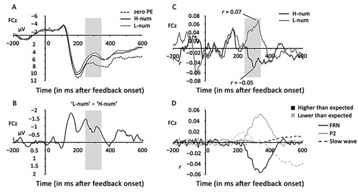
Event-related potential (ERP) results of Experiment 2 at the fronto-central (FCz) site. (A) shows apparent negative-going waves within the 240–340-ms time window (shaded area). (B) describes the negativity produced by subtracting the waveform of H-num from that of L-num within the 240–340-ms time window (shaded area). (C) shows the single-trial Pearson correlations between the trial-wise PE and feedback-related potentials. Significant correlations were observed within the 240–340-ms time window (shaded area). (D) shows the principal components analysis (PCA) factors extracted from the preceding correlation waveforms. All factors are denoted in unit r against time and plotted separately for higher- and lower-than-expected numbers.
Correlation Results
The single-trial Pearson correlations between the trial-wise PE and feedback-related potentials (Fig. 5C) revealed a significant negative correlation for H-num (r = −0.05 ± 0.12; t27 = −2.16, P = 0.04) but a significant positive correlation for L-num (r = 0.07 ± 0.12; t27 = 2.97, P = 0.006). This experiment adopted pure digital feedback that excluded the reward effect and demonstrated that the feedback-related potentials were parametrically modulated by a reward-independent expectancy violation (cf. the UPE encoder in Fig. 1A).
PCA Components
The two-step PCA performed on the preceding correlation waveforms resulted in a total of 33 temporospatial factors. The first three factors are listed in Table 3 and plotted in Fig. 5D.
The factor TF2/SF1 resembled FRN features. The one-sample t-test on this factor’s peak amplitude revealed a significant negative correlation for H-num (t27 = −2.89, P = 0.008) but a significant positive correlation for L-num (t27 = 3.55, P = 0.001), which validated the preceding correlation waveforms. The temporal and spatial features of the factor TF3/SF1 resembled the P2 component, which showed nonsignificant correlations for both H-num (t27 = 0.26, P = 0.797) and L-num (t27 = 1.58, P = 0.126). Finally, factor TF1/SF1 showed a similar profile to that of slow wave, displaying a nonsignificant correlation for H-num (t27 = 0.68, P = 0.5) but a significant negative correlation for L-num (t27 = −2.36, P = 0.026).
Discussion of Experiment 2
In Experiment 2, the digital feedback was merely indicative of participants’ predictive accuracy, which conveyed expectancy violation but removed reward signal. Accordingly, the UPE encoder in Experiment 1 could be strictly tested here. As in Experiment 1, the results showed that the participants developed a gradual discrimination of two shapes as the task progressed (Fig. 4A). Furthermore, the expected number of high-number shape was significantly higher than that of low-number shape even in the first phase, suggesting that association learning was much easier with fixed associations.
Then, apparent negative-going ERP waves were found, of which the H-num waveform was more positive than L-num waveform, manifesting a significant negativity when subtracting the waveform of H-num from that of L-num (Fig. 5A and B). Although this negativity seemed similar to the FRN derived by subtracting the waveform of +PEs from that of –PEs, it was intrinsically irrelevant to the outcome valence (RPE) because the feedback in Experiment 2 was only indicative of predictive accuracy. The more negative waveform induced by L-num was consistent with the findings in Experiment 1, where the waveforms of lower-than-expected outcomes (L-gain, L-loss) were also more negative than those of higher-than-expected outcomes (H-gain, H-loss), which suggests that the responses to positive and negative expectancy violation were neither monotonic nor symmetric. The further correlation and PCA analyses revealed that the correlation between the trial-wise PE and feedback-related potentials was negative for H-num but positive for L-num (Fig. 5C and D). This response pattern was clearly consistent with the UPE encoder.
Experiment 3
The converging results of Experiments 1 and 2 suggest that the missing RPE encoder in Experiment 1 was due to the de-emphasis of outcome valence and that the observed UPE encoders reflected the attention to predictive accuracy. It seems that a heterogeneous emphasis of these dimensions may lead to different responses. To examine this assumption, we conducted Experiment 3, which was identical to Experiment 1 (gain and loss domains) in all aspects except that some blocks emphasized outcome valence while others highlighted predictive accuracy. We predicted that an RPE encoder would be observed when emphasizing outcome valence while a UPE encoder would be found when highlighting predictive accuracy.
PCA factors extracted from the preceding correlation waveforms for statistical analysis in Experiment 2
| Proposed component | Factor | Temporal peak (ms) | Spatial peak | Variance explained (%) |
|---|---|---|---|---|
| Slow wave | TF1/SF1 | 564 | P2 | 8.43 |
| FRN | TF2/SF1 | 334 | P3 | 9.76 |
| P2 | TF3/SF1 | 226 | FC1 | 3.26 |
| Proposed component | Factor | Temporal peak (ms) | Spatial peak | Variance explained (%) |
|---|---|---|---|---|
| Slow wave | TF1/SF1 | 564 | P2 | 8.43 |
| FRN | TF2/SF1 | 334 | P3 | 9.76 |
| P2 | TF3/SF1 | 226 | FC1 | 3.26 |
Materials and Methods
Participants
Thirty-five participants were recruited from Southwest University (China) for monetary compensation. All the participants were right-handed and had normal or corrected-to-normal vision. None reported any psychiatric, neurological, or medical illness. Ten participants were dismissed: one for incomplete recordings, four for excessively large artifacts on EEG signals, and five for misunderstanding the task rule (concentrating on outcome valence or predictive accuracy in all blocks); the remaining 25 participants underwent analysis for the valence blocks (9 males, 19.76 ± 1.13 years old) and predictive-accuracy blocks (10 males, 20.16 ± 1.60 years old). The participants provided written consent upon their arrival. The study was approved by the Human Ethics Committee of Southwest University and complied with the Helsinki Declaration guidelines.
Stimuli and Procedure
The experimental procedure was the same as in Experiment 1. Notably, in valence blocks, the participants were explicitly told that they simply needed to focus on outcome valence while the accuracy of their predictions could not affect the outcomes. However, in the predictive-accuracy blocks, the participants were told that the outcome was dependent only on predictive accuracy. To maintain balance with valence blocks, the predictive-accuracy blocks also included gain and loss domains. Specifically, in the gain domain, the participants were given a basic amount (15) in each trial, and the final gain was the difference between this amount and PE (actual value minus expected value). Therefore, the more accurate the prediction, the more money was retained. In the loss domain, no basic amount was provided, and the difference between actual and expected values was the money they lost in actuality; similarly, the more accurate the prediction, the less money was lost.
The whole experiment included eight blocks each for the valence and predictive-accuracy blocks, half of which was for the gain domain and the other half for the loss domain (40 trials per block, 640 trials in all). The sequence for valence and predictive-accuracy block was counterbalanced among participants. This experiment involved 32 shapes, with two unique shapes for each block. To facilitate real learning, the high- and low-value shapes were truly related with higher (>10) and lower feedback (≤10), respectively. After the experiment, each participant was paid 80 RMB in addition to a performance-dependent bonus of 0–20 RMB. The entire experiment lasted about 100 minutes.
EEG Recording and Preprocessing
EEG acquisition here was the same as in Experiment 1.
Behavioral Analysis
Behavioral analyses were the same as those in Experiment 1. Notably, in the predictive-accuracy blocks, because the response patterns were similar between the gain and loss domains upon the inspection of results, the two domains were integrated.
ERP Analysis
The ERPs were created and analyzed same as those in Experiment 1. By subtracting the expected values from the actual values, six types of trials were created for valence blocks: expected gain (zero PE), higher-than-expected gain (H-gain: +PE), lower-than-expected gain (L-gain: –PE), expected loss (zero PE), higher-than-expected loss (H-loss: –PE), and lower-than-expected loss (L-loss: +PE). Furthermore, three types of trials were created for the predictive-accuracy blocks: expected amount (zero PE), higher-than-expected amount (H-amount), and lower-than-expected amount (L-amount). After excluding trials associated with EEG artifacts, 92.51% of the trials were retained for the gain domain and 89.26% for the loss domain, while 92.63% of the trials remained for the predictive-accuracy blocks.
Correlation Analysis
The single-trial Pearson correlation analysis was the same as that in Experiment 1.
PCA
Similar to Experiment 1, a two-step PCA was performed on the correlation waveforms. In the valence blocks, the temporal PCA produced 15 temporal factors, and 45 temporospatial factors were produced after spatial PCA; in the predictive-accuracy blocks, 13 temporal factors were produced by temporal PCA, and 39 temporospatial factors were produced after spatial PCA.
Results
Behavioral Results
In both valence (Fig. 6A) and predictive-accuracy blocks (Fig. 6B), the participants’ expected value for the high-value shape was not different from that for the low-value shape at the start, but as the task progressed, it became significantly higher than the expected value for low-value shape, demonstrating a progressive discrimination between the two shapes. Subsequently, continuous PEs ranging from −20 to 20 were plotted in Fig. 6C for the gain (skewness = 0.006, kurtosis = −0.58), loss (skewness = −0.07, kurtosis = −0.63), and predictive-accuracy blocks (skewness = −0.009, kurtosis = −0.60), showing approximately normal distributions. Finally, Pearson correlations between the adjustment size of prediction (predictionN − predictionN − 1) and the PE of trial N − 1 were significant for high- (across subjects: r = 0.90, P < 0.0001; mean r = 0.66) and low-value shapes (across subjects: r = 0.93, P < 0.0001; mean r = 0.57) in the gain domain (Fig. 7A) and significant for high- (across subjects: r = 0.84, P < 0.0001; mean r = 0.50) and low-value shapes (across subjects: r = 0.91, P < 0.0001; mean r = 0.64) in the loss domain (Fig. 7B) as well as significant for high- (across subjects: r = 0.94, P < 0.0001; mean r = 0.74) and low-value shapes (across subjects: r = 0.96, P < 0.0001; mean r = 0.74) in the predictive-accuracy blocks (Fig. 7C).
Development of participants’ expected values for high- and low-value shapes throughout the block in Experiment 3. In both valence blocks (A) and the predictive-accuracy task (B), the participants progressively discriminated between the two shapes as the task progressed. (C) reflects approximately normal distributions of PEs for gain, loss, and the predictive-accuracy task in Experiment 3. The error bar denotes standard errors, * denotes P < 0.05, ** denotes P < 0.01, and *** denotes P < 0.001.
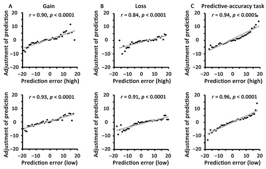
Correlations between the adjustment size of prediction (predictionN − predictionN − 1) and PE of trial N − 1 for high- and low-value shapes in Experiment 3. The scatterplots show across-subjects correlations for gain (A), loss (B), and the predictive-accuracy task (C).
ERP Results
The ERPs were created, showing apparent negative-going waves (Fig. 8) in the 240–340 ms time window at the FCz site for gain (F2 = 6.11, P = 0.013), loss (F2 = 2.13, P = 0.151), and the predictive-accuracy task (F2 = 25.48, P < 0.0001). Specifically, in valence blocks, the expected-gain waveform (zero PE; mean = 8.73 μV) did not differ from the H-gain waveform (mean = 8.58 μV; t24 = 0.18, P = 0.857) but was significantly more positive than the L-gain waveform (mean = 6.38 μV; t24 = 2.48, P = 0.02); meanwhile, the H-gain waveform was significantly more positive than the L-gain waveform (t24 = 5.29, P < 0.0001). In the loss domain, the waveform of expected loss (zero PE; mean = 9.64 μV) was not different from those of H-loss (mean = 7.77 μV; t24 = 1.70, P = 0.101) and L-loss (mean = 8.86 μV; t24 = 0.75, P = 0.463), but the waveform of H-loss was significantly more negative than that of L-loss (t24 = 2.48, P = 0.021). In the predictive-accuracy blocks, the expected-amount waveform (zero PE; mean = 10.75 μV) was significantly more positive than the H-amount (mean = 7.99 μV; t24 = 3.93, P = 0.001) and L-amount waveforms (mean = 6.77 μV; t24 = 6.35, P < 0.0001), and the H-amount waveform was significantly more positive than the L-amount waveform (t24 = 4.02, P < 0.0001).
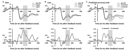
Event-related potential (ERP) results in Experiment 3 at the fronto-central (FCz) site within the 240–340-ms time window (shaded area). (A) describes apparent negative-going waves in the gain domain; a significant negativity was revealed by subtracting the waveform of H-gain from that of L-gain. (B) describes apparent negative-going waves in the loss domain; a significant negativity was found by subtracting the waveform of L-loss from that of H-loss. (C) describes apparent negative-going waves in the predictive-accuracy task; a significant negativity was found by subtracting the waveform of H-amount from that of L-amount.
In the valence blocks, by subtracting the waveform of +PEs from that of –PEs, significant negativities were revealed in both gain (t24 = −5.29, P < 0.0001) and loss domains (t24 = −2.48, P = 0.021); moreover, a significant negativity (t24 = −4.81, P < 0.0001) was observed when subtracting the waveform of +PEs from that of –PEs across two domains (Fig. S1C). In the predictive-accuracy blocks, a significant negativity was found by subtracting the H-amount waveform from the L-amount waveform (t24 = −4.02, P < 0.0001).
Because the zero-PE waveform was more positive than other conditions in the three experiments, we also computed additional difference waves for each experiment by subtracting the zero-PE waveform from those of higher- and lower-than-expected outcomes, respectively (Fig. S2). In Experiment 1, we observed significant negativities for both H-gain (t22 = −3.26, P = 0.004) and L-gain (t22 = −5.33, P < 0.0001); in the loss domain, we found no significant result for H-loss (t22 = −1.37, P = 0.186) but observed a significant negativity for L-loss (t22 = −2.13, P = 0.045). In Experiment 2, significant negativities were found for both H-num (t27 = −3.00, P = 0.006) and L-num (t27 = −4.22, P < 0.0001). Finally, for the valence blocks in Experiment 3, we only found a significant negativity for L-gain (t24 = −2.48, P = 0.02); for the predictive-accuracy blocks, significant negativities were found for both H-amount (t24 = −3.93, P = 0.001) and L-amount (t24 = −6.35, P < 0.0001).
Correlation Results
In the valence blocks (Fig. 9A and B), the single-trial Pearson correlation revealed a significant positive correlation for L-gain (r = 0.12 ± 0.13; t24 = 4.71, P < 0.0001) but a nonsignificant correlation for H-gain (r = −0.03 ± 0.14; t24 = −1.07, P = 0.295); moreover, a significant negative correlation was observed for H-loss (r = −0.06 ± 0.14; t24 = −2.24, P = 0.035) but no significant correlation was found for L-loss (r = −0.05 ± 0.21; t24 = −1.33, P = 0.197). Furthermore, the predictive-accuracy blocks (Fig. 9C) showed a nonsignificant correlation for H-amount (r = −0.03 ± 0.10; t24 = −1.59, P = 0.124) but a significant positive correlation for early L-amount (r = 0.09 ± 0.09; t24 = 5.13, P < 0.0001), while a marginally significant negative correlation was observed for late L-amount (r = −0.05 ± 0.13; t24 = −2.05, P = 0.051).

Correlation waveforms of Experiment 3 at the fronto-central (FCz) site within the 240–340-ms time window (shaded area) are plotted at the upper panel for gain (A), loss (B), and the predictive-accuracy task (C). The PCA factors extracted from the preceding correlation waveforms are plotted for each task at the lower panel. All factors are denoted in unit r against time.
PCA Components
The two-step PCA performed on the preceding correlation waveforms resulted in 45 temporospatial factors for the valence blocks and 39 temporospatial factors for the predictive-accuracy blocks. The first three factors of each condition are listed in Table 4 and plotted in Fig. 9.
PCA factors extracted from the preceding correlation waveforms for statistical analysis in Experiment 3
| Proposed component | Factor | Temporal peak (ms) | Spatial peak | Variance explained (%) |
|---|---|---|---|---|
| Valence blocks | ||||
| Slow wave | TF1/SF1 | 566 | CP2 | 10.70 |
| FRN | TF2/SF1 | 280 | C4 | 5.27 |
| P3 | TF3/SF1 | 364 | C1 | 4.51 |
| Predictive-accuracy blocks | ||||
| Slow wave | TF1/SF1 | 562 | P1 | 10.44 |
| FRN | TF2/SF1 | 304 | Cz | 7.18 |
| P3 | TF3/SF1 | 394 | C2 | 5.79 |
In the valence blocks, factor TF2/SF1 resembled FRN features. The one-sample t-test on this factor’s peak amplitude revealed a nonsignificant correlation for H-gain (t24 = −0.78, P = 0.445) but a significant positive correlation for L-gain (t24 = 5.25, P < 0.0001); in the loss domain, no significant correlation was observed for H-loss (t24 = −0.43, P = 0.673) or L-loss (t24 = −0.56, P = 0.580). The second factor, TF3/SF1, resembled the features of the P3 component, which did not exhibit any significant correlation under all conditions. Finally, factor TF1/SF1 showed a profile similar to that of slow wave, which displayed a significant positive correlation for H-gain (t24 = 2.17, P = 0.04) but a negative correlation for L-gain (t24 = −2.11, P = 0.045); this factor also showed a significant positive correlation for H-loss (t24 = 4.01, P = 0.001) but a nonsignificant correlation for L-loss (t24 = −1.66, P = 0.11).
In the predictive-accuracy blocks, factor TF2/SF1 resembled FRN features, which showed nonsignificant correlations for both H-amount (t24 = −0.91, P = 0.373) and L-amount (t24 = −0.38, P = 0.707). Furthermore, factor TF3/SF1 resembled the features of the P3 component, but no significant correlation was found for both H-amount (t24 = −0.84, P = 0.411) and L-amount (t24 = −1.13, P = 0.27). Finally, factor TF1/SF1 resembled the features of slow wave, which displayed a significant positive correlation for H-amount (t24 = 2.57, P = 0.017) but a negative correlation for L-amount (t24 = −3.56, P = 0.002).
Discussion of Experiment 3
The participants also developed gradual discrimination between two shapes as the task proceeded in both valence (Fig. 6A) and predictive-accuracy blocks (Fig. 6B). Critically, in the predictive-accuracy blocks, the expected value of the high-value shape was significantly higher than that of the low-value shape in the second phase, which was much earlier than in the valence blocks. Thus, all three experiments consistently validated that the evaluation of numerical size was easier than that of outcome valence.
As expected, the ERP results showed that in the valence blocks, the H-gain waveform (+PE) was more positive than the L-gain waveform (–PE), whereas the L-loss waveform (+PE) was more positive than the H-loss waveform (–PE); by subtracting the waveform of +PEs from that of –PEs, significant negativities were found in both domains (Fig. 8A and B), which was consistent with RL–RPE theory. In the predictive-accuracy blocks, the H-amount waveform was more positive than the L-amount waveform, exhibiting a significant negativity when the former was subtracted from the latter (Fig. 8C). This result was in accordance with the ERP results of Experiments 1 and 2, which again suggested that the responses to positive and negative violation of expectancy were neither monotonic nor symmetric.
The single-trial correlation and PCA procedure further showed that in the valence blocks, the PEs were positively correlated with the L-gain waveform but were negatively correlated with the H-loss waveform (Fig. 9A and B). Although no significant correlations were observed for H-gain and L-loss, these responses could not be considered as UPE encoders because of the opposite responses of feedback-related potentials between the appetitive and aversive domains. We speculate that the significant correlations for –PEs (L-gain and H-loss) may be due to the “loss aversion” effect (Kahneman and Tversky 1979; Tom et al. 2007) in which the participants exhibited more sensitivity to negative-valence PEs; conversely, the +PEs (H-gain and L-loss) were less sensitive and thus elicited a weaker or nonsignificant modulation of positive-valence PEs on feedback-related potentials. In the predictive-accuracy blocks, the PEs were positively correlated with the L-amount waveform at an early stage but were negatively (albeit nonsignificantly) correlated with the H-amount waveform (Fig. 9C). Likewise, the absence of a significant correlation for H-amount may be caused by positive PEs being less sensitive. In all three experiments, when participants were more focused on predictive accuracy, the waveforms of the lower-than-expected outcomes were consistently found to be more negative than those of the higher-than-expected outcomes, implying that the lower-than-expected outcomes (negative deviation from the expectation) may be coded in the same manner as negative-valence events and thus recruited more sensitivity, while the higher-than-expected outcomes (positive deviation from the expectation) were less sensitive and showed weaker or nonsignificant PE modulation on ERPs.
General Discussion
The current study investigated how feedback-related potentials responded to the valence of outcome and/or its violation from expectancy. Experiment 1 adopted monetary gain and loss as feedback, which indicated both outcome valence and predictive accuracy; Experiment 2 simply included pure digital feedback to examine the predictive-accuracy effect. The same results revealed in these two experiments suggested that the UPE encoder in Experiment 1 was due to the sole effect of predictive accuracy when the outcome valence was obscured. Thereafter, to clearly separate and identify the effects of outcome valence and predictive accuracy, we conducted Experiment 3, which was identical to Experiment 1 except that some blocks emphasized the outcome valence while others highlighted predictive accuracy. As hypothesized, a similar UPE encoder was found when predictive accuracy was emphasized, but an RPE encoder was observed when valence was highlighted. Therefore, we suggest that feedback-related potentials reflect the outcome valence as well as its violation from expectancy, exhibiting preferential response depending on the highlighted dimension.
Behaviorally, all three experiments consistently validated participants’ gradual discrimination of the associations between shapes and feedback as they learned those associations, and such learning was faster for the evaluation of predictive accuracy than that of outcome valence. Strikingly, significant correlations were observed between prediction adjustment and the PEs encountered ahead for that shape, which confirmed that the PEs were taken as learning signals to promote the adjustment of expectations. These results also suggested that our PEs, calculated between the actual feedback and the participants’ subject ratings, were effective in forming associative learning, thereby refuting the possibility that the overtly reported ratings might cause a deviation to their real predictions, which are usually inferred using computational models (Philiastides et al. 2010; Cazé and van der Meer 2013; Sambrook and Goslin 2016). Noticeably, those models are mostly computed in a reward frame with “all-or-nothing” outcomes and thus are inappropriate for the loss frame as well as for our varying feedback.
On ERPs, for missing RPEs in Experiment 1, we presumed that the participants were mainly concerned with the predictive accuracy given the high difficulty of the task, which would obscure feedback valence and result in similar feedback-related potentials in the appetitive and aversive domains as in previous studies (Talmi et al. 2013; Huang and Yu 2014). This assumption was clearly validated by the same results of Experiment 2 and the predictive-accuracy blocks in Experiment 3, which simply reflected the effect of predictive accuracy. However, upon highlighting the outcome valence, the worse-than-expected outcomes (L-gain, H-loss) elicited more negative waveforms than better-than-expected outcomes, which was consistent with RL–RPE theory (Gehring and Willoughby 2002; Holroyd and Coles 2002). These results show that the controversial findings of previous studies may be attributed to the heterogeneity of the highlighted dimension. In addition, when participants were concerned with predictive accuracy (Experiments 1 and 2 and the predictive-accuracy blocks in Experiment 3), the waveforms of the negative expectancy violation (lower-than-expected outcomes) were consistently more negative than those of the positive expectancy violation (higher-than-expected numbers). The participants might code negative expectancy violations as negative-valence outcomes, which usually recruited more sensitivity because of the aversion of negative events (Kahneman and Tversky 1979; Koebberling and Wakker 2005; Blavatskyy 2011), yielding more negative waveforms than positive events.
Although both RPE and UPE theories state that the FRN amplitude is proportional to PEs, only a few studies have investigated the PE’s quantitative modulation on FRN. Therefore, in this study, we calculated the correlation coefficients between the trial-wise PE and feedback-related potentials and found a positive correlation for lower-than-expected gain in the valence blocks of Experiment 3, which suggested that the feedback-related potentials were more negative with the increasing degree to which gains were lower than expected. Furthermore, we observed a negative correlation for higher-than-expected loss, suggesting that the feedback-related potentials were more negative with the increasing degree to which losses were higher than expected (cf. the RPE encoder in Fig. 1A). In other conditions that merely reflected the predictive-accuracy effect, the positive correlations for lower-than-expected outcomes indicated that the increasing negative expectancy violation was associated with more negative waveform, while the negative correlations for higher-than-expected outcomes indicated that the increasing positive expectancy violation was associated with more negative waveform (UPE encoder). Despite these findings, no significant correlation was observed for +PEs (H-gain, L-loss) in the valence blocks of Experiment 3 and for positive expectancy violation in Experiment 1 (H-loss) and the predictive-accuracy blocks in Experiment 3 (H-amount). The absence of correlations in these trials may be attributed to the fact that less sensitivity is recruited by positive-valence outcomes and positive expectancy violation (Murata 2015). Additionally, unlike the significant negative correlation observed for H-num in Experiment 2, where the feedback purely indicated predictive accuracy, the nonsignificant correlations for H-loss in Experiment 1 and for H-amount in Experiment 3 may also be due to the task’s complexity (compound of outcome valence and predictive accuracy) that would attenuate the differences among those PE values, exhibiting a weak PE size effect (Cockburn and Holroyd 2018).
Accordingly, we suggest that the RPE and UPE encoders are reconcilable. Specifically, the negative-going waveforms in Experiments 1 and 2 as well as in the predictive-accuracy blocks of Experiment 3, which reflected sensitivity to expectancy violation, resembled the feature of N200, a negativity that is usually elicited by unexpected and task-relevant deviated stimuli (Folstein and Van Petten 2008). Thus, the UPE encoder during FRN interval might be a special case of N200 when only the reward-independent expectancy violation was emphasized. However, when the reward effect was highlighted, it interacted with expectedness and produced an FRN according to RL–RPE (as in the valence blocks in Experiment 3). This interpretation is in line with the view that the unexpected no-reward would elicit N200 (baseline), but the unexpected reward would elicit a positivity that attenuates N200, leading to the observed difference wave between favorable and unfavorable outcomes (Holroyd et al. 2008; Baker and Holroyd 2011; Holroyd et al. 2011; Proudfit 2015).
The RPE and UPE encoders can be attributed to the two neuromodulatory systems implicated in reward learning and decision-making: the midbrain dopaminergic (DA) system and the locus coeruleus–norepinephrine (LC–NE) system. The midbrain DA system is relevant to reward and RPE processing (Lammel et al. 2014; Chau et al. 2018); some dopamine neurons are also associated with salience encoding (Bromberg-Martin et al. 2010). The LC–NE system is sensitive to expectancy violation and salient stimuli (Aston-Jones and Cohen 2005; Nieuwenhuis et al. 2005a; Warren and Holroyd 2012). Therefore, we presume that the partial DA system and the LC–NE system will react to expectancy violations and induce an N200-like negativity; furthermore, these two systems may cooperate to support motivational learning when the reward effect interacts with expectedness, eliciting an FRN (difference wave) as asserted by RL–RPE (Warren and Holroyd 2012).
Similar to Sambrook and Goslin’s (2016) method, we adopted a temporospatial PCA approach on correlation waveforms to separate potential overlapping components. In most conditions, the FRN component was similar to the preceding correlation waveform, although it was irresponsive to +PEs or –PEs in some cases. Because the three experiments reflected various aspects of feedback processing (Sambrook and Goslin 2015), the absence of FRN component for +PEs or –PEs may be due to that in different tasks, diverse factors would influence the underlying processing mechanism to varying degrees. Sambrook and Goslin (2016) also merely revealed a + PE encoder. Apart from the varying impact of different factors on feedback processing, the diverse results in previous PCA studies (Holroyd et al. 2008; Foti et al. 2011; Sambrook and Goslin 2016) also suggest a large variation in PCA procedures, and thus, great caution must be exercised when considering PCA results. Other components resembling P2, P3, and later slow wave were also revealed. These components were demonstrated to be responsive to expectancy violation (Courchesne et al. 1977; Hajcak et al. 2007) and reward valence (Holroyd 2004). In particular, the P3 is an ERP component that overlaps the temporal interval of FRN, which is usually sensitive to infrequent events (Yeung and Sanfey 2004; Hajcak et al. 2005).
Finally, because our feedback probabilities were unchanged, one might argue that the feedback was not unexpected. If so, “zero PE” was highly unexpected because of its extremely low frequency and should induce more negative waveforms. However, this assumption was refuted since the fully expected condition’s waveform was almost the most positive. Another possibility was that “zero PE” would result in an intrinsic reward signal for correct prediction. To demonstrate this hypothesis, the “zero PE” waveform was subtracted from those of –PEs and + PEs, respectively, which revealed significant negativities, particularly in Experiments 1 and 2 and the predictive-accuracy blocks in Experiment 3, where the participants were mainly focused on predictive accuracy. Correct prediction (zero PE) seemed to behave as +PEs, eliciting more positive waveforms than the other two conditions that involved expectancy violations. The difference between zero PE and a positive or negative expectancy violation was analogous to that between the +PEs and –PEs as RL theory proposes. Moreover, in the valence blocks of Experiment 3, correct prediction might lead to a reward effect similar to that of H-gain and L-loss, exerting more positive waveforms than L-gain and H-loss (although nonsignificant). Therefore, the valence effect may have occurred during the feedback processing all along due to the reward signal incurred by the correct prediction. Because the valid trials for “zero PE” were miniscule in all three experiments, future studies should use more trials to examine this assumption.
Through three successive experiments, we demonstrate that feedback-related ERPs respond to both the outcome valence and its expectancy violation, exhibiting a preferential response depending on which dimension is emphasized. Specifically, a UPE encoder was revealed when only predictive accuracy was highlighted while an RPE encoder was found when the reward effect was salient and interacted with expectedness. This study adds to the present understanding of the controversial findings in previous studies and provides more holistic knowledge concerning feedback-related ERPs.
Funding
The National Natural Science Foundation of China (61431013, 31771254); the Fundamental Research Funds for the Central Universities (SWU1609106, SWU1709107, and SWU1909567).
Notes
We are grateful to Dr Tobias Egner for his helpful discussions of data analyses and writing. We also thank Jeremy Goslin for generously sharing the single-trial correlation code. Conflict of Interest: None declared.
Author Contributions
Y.G. and A.C. designed the study. Y.G., X.Z., Q.L., and N.H. performed the experiment. Y.G., T.L., and X.Z. analyzed the data. Y.G., Y.Z., and A.C. wrote the manuscript.