


Abstract
The connectivity of cortical microcircuits is a major determinant of brain function; defining how activity propagates between different cell types is key to scaling our understanding of individual neuronal behavior to encompass functional networks. Furthermore, the integration of synaptic currents within a dendrite depends on the spatial organization of inputs, both excitatory and inhibitory. We identify a simple equation to estimate the number of potential anatomical contacts between neurons; finding a linear increase in potential connectivity with cable length and maximum spine length, and a decrease with overlapping volume. This enables us to predict the mean number of candidate synapses for reconstructed cells, including those realistically arranged. We identify an excess of potential local connections in mature cortical data, with densities of neurite higher than is necessary to reliably ensure the possible implementation of any given axo-dendritic connection. We show that the number of local potential contacts allows specific innervation of distinct dendritic compartments.
Introduction
The functionality of the brain depends fundamentally on the connectivity of its neurons for everything from the propagation of afferent signals (Matthews and Fuchs 2010; Oh et al. 2014) to computation and memory retention (Hebb 1949; Hopfield 1984; Abbott and Regehr 2004). Connectivity arises from the apposition of complex branched axonal and dendritic arbors which each display a diverse array of forms, both within and between neuronal classes (Bok 1936; Sholl 1953; Ascoli et al. 2007; Ascoli et al. 2008). Despite this complexity, neurons of different classes have been observed to form synapses in highly specific ways, leading to potentially highly structured connectivity motifs within neuronal networks (Binzegger 2004; Yoshimura and Callaway 2005; Ohki and Reid 2007; Perin et al. 2011; Potjans and Diesmann 2014; Jiang et al. 2015).
Whilst the large-scale EM studies necessary to definitively constrain synaptic connectivity remain prohibitively slow (Briggman and Denk 2006; da Costa and Martin 2013; Helmstaedter 2013) and viral synaptic tracing is limited to small numbers of neurons (Wall et al. 2013), potential synaptic locations from the close juxtaposition of dendrite and axon are more readily measured (Markram et al. 1997; Lee et al. 2016) and provide the potential set of all possible synaptic contacts; the backbone upon which neuronal activity can fine tune functional connectivity. A number of studies (Silver 2003; Biró et al. 2005, 2006) have also combined paired-cell electrophysiology with light- and electron-microscopy to relate functional with potential connectivity, allowing direct investigation of the relationship between identified anatomical contacts and neurotransmitter vesicle release. It has been shown that much of the specificity in potential connectivity can be explained by a detailed analysis of the statistical overlap of different axonal and dendritic arbors (Hill et al. 2012; Markram et al. 2015; Reimann 2017), although such techniques are again insufficient to produce a functional connectome and lack many crucial biological details (Jiang et al. 2015; Villa et al. 2016; Sancho and Bloodgood 2018). However, even such analyses rely on full neuronal reconstructions with large numbers of parameters and are difficult to apply intuitively to microcircuits; there is value in a simple and easily interpretable description of the expected connectivity between a given pair of cells.
The fundamental assumption here is a form of Peters’ Rule, where synapses form uniformly where possible (Peters and Feldman 1976; Braitenberg and Schüz 1998). Peters’ rule has been interpreted in a number of different ways at a number of different scales; from predicting of the connectivity between different neuronal classes from their relative abundance (Li et al. 2007) to estimating the number of synapses between a given pair of neurons (Packer et al. 2013). There is experimental evidence both for and against the assumption of uniform synapse formation in different brain regions, species, and under different experimental protocols. Some cell types, such as inhibitory cortical chandelier cells, specifically target a region of the postsynaptic cell, in this case the axon initial segment of pyramidal neurons, and so violate Peters’ Rule in the strict sense. A recent review by Rees et al. (2017) summarizes the experimental evidence for (Packer et al. 2013; van Pelt and van Ooyen 2013; Merchán-Pérez et al. 2014; Rieubland et al. 2014) and against (Mishchenko et al. 2010; Potjans and Diesmann 2014; Kasthuri et al. 2015; Lee et al. 2016) Peters’ Rule at the level of individual neurites; but in general, it seems that uniform potential structural connectivity is an accurate and powerful model for large regions of the central nervous system.
Given a backbone of neurite structure, neuronal activity is able to strengthen or weaken synapses; allowing memory formation (Hebb 1949), changes in information storage capacity (Stepanyants et al. 2002; Chklovskii et al. 2004), and sensory tuning (Lee et al. 2016). This relies on the relative dynamism of spine growth and retraction, which occurs on timescales of minutes (Lendvai et al. 2000) (although actual synapse formation can be slower; Knott et al. 2002), compared with neurite remodeling, which is typically stable over timescales of weeks or months in mature cells (Trachtenberg et al. 2002; Chow et al. 2009). Such a structural backbone is a step towards, and an important constraint on, understanding the functional connectome; which cells are connected, how strongly, and with what short-term plasticities on what timescales.
Spine production and elimination vary between brain areas (Huttenlocher and Dabholkar 1997) and change with development, with a relatively large number of contacts forming at early developmental stages (Huttenlocher 1979; Rakic et al. 1986; Innocenti and Price 2005) and being maintained over long periods (Bourgeois et al. 1994; Petanjek et al. 2011) by selective stabilization (Changeux and Danchin 1976) and balanced elimination (Purves and Lichtman 1980; Rakic and Riley 1983; Villa et al. 2016). Synaptic stabilization also depends on neuron type and whether contacts are formed directly onto the dendritic shaft or spine (Bourgeois et al. 1994; Sancho and Bloodgood 2018), and interacts with longer term changes in neurite structure (Innocenti 1981; Petanjek et al. 2008; Innocenti and Caminiti 2017). Dynamism in synaptic formation is strongly associated with learning in a rich environment (Rakic et al. 1994; Petanjek et al. 2011), having a high number of close appositions between axons and dendrites of given cell types creates more potential for dynamic changes in connectivity.
The proportion of close appositions that appears to be bridged by spines at a given time is traditionally referred to as the filling fraction (Stepanyants et al. 2002) and original estimates ranged from 0.1 (macaque V1 visual cortex) to just under 0.4 (rat CA3 hippocampus). A further detail comes from the relationship between the number of anatomical contacts seen under light microscopy with those with synaptic structure under an electron microscope; Markram et al. (1997) investigated thick-tufted layer 5 pyramidal cells in rat somatosensory cortex and found that when an axon passed close to a dendrite and displayed substantial swelling indicative of a bouton, then ~80% were true synaptic contacts. Such a reliable and consistent, but not perfect, relationship has since been observed in different neuronal systems (Feldmeyer et al. 1999; Feldmeyer et al. 2002; Mishchenko et al. 2010). Stepanyants et al. (2008) investigated potential contacts within the cat visual cortex and showed that all-to-all connectivity within local circuits (to a distance of 200 μm) could be implemented from bridging close appositions. More recent studies have found, as we observe here in the adult mouse visual cortex dataset of Jiang et al. (2015), lower proportions of functional to potential contacts (Kasthuri et al. 2015; Lee et al. 2016). The excess of potential connectivity arises from the extensive branching of cortical neurites and raises questions about the additional functionality provided by this additional metabolic expenditure.
On the postsynaptic side, dendritic trees act as a filter on inputs. The passive electrotonic properties of dendritic cables cause synaptic currents to decay in time and space (Rall 1964), whilst active processes (Llinas 1988; Schiller et al. 2000) act to amplify integrated signals that locally exceed a threshold. Inputs to specific regions of some cells allow nonlinear computations to be performed at an intraneuron scale (Mel 1993; Poirazi et al. 2003; Polsky et al. 2004; London and Häusser 2005; Losonczy and Magee 2006). The interaction of clustered or distributed excitatory (Behabadi et al. 2012) and inhibitory (Gidon and Segev 2012) inputs within a dendritic tree mean that a subcellular-resolution connectome is relevant to realistic network function.
We investigate how well the number of potential synaptic contacts between pairs of neurons can be predicted from simple and intuitive properties of the spatial overlap of their neurite arbors. We find an excess of local potential connectivity, both predicted and measured, beyond that described by Stepanyants et al. (2002) and more than sufficient to reliably implement all possible connections at the level of single cells. We investigate further how well this allows for specific connectivity at the subcellular level of dendritic compartments.
Materials and Methods
Data and Algorithm Availability
All simulations were done in MATLAB (ver. 2018b) using the TREES toolbox (ver. 1.15) and custom scripts. The morphologies used in the paper were downloaded from NeuroMorpho.Org (www.neuromorpho.org; Ascoli et al. 2007) and the Cell Types database of the Allen Institute for Brain Science (Allen Brain Institute 2015) with sources indicated in Table 3. Selection of cells and preprocessing for the morphologies in Figure 5 were performed using the Allen Software Development Kit (freely available at http://alleninstitute.github.io/AllenSDK/install.html) in a Jupyter Notebook (ver. 5.5) running Python (ver. 3.7). All data and code necessary to reproduce the figures and tables in the paper are included as Supplementary File 2.
Of particular general utility are the following new MATLAB Trees Toolbox functions:
dscam_tree—Applies the Down Syndrome Cell Adhesion Molecule (DSCAM) null algorithm (described below) to a tree to produce clustered dendrites.
M_atten_tree—Estimates the number of dendritic compartments based on electrotonic attenuation.
peters_tree—Determines the number of potential anatomical contacts between two neurites.
share_boundary_tree—Determines the boundary of the overlap of two neurites and their respective lengths within this region.
Generalized Minimum Spanning Trees
Synthetic neurites are produced using the generalized minimum spanning tree (MST) algorithm described by Cuntz et al. (2010) and available as part of the Trees Toolbox package for MATLAB. Typically, neurites are simulated by uniformly randomly distributing a number of points in a cube with sides of length 200 μm and connecting them into a generalized MST using the Trees Toolbox function MST_tree. The number of points for both the axonal and dendritic trees is typically taken to be 65, the trees are generated in cubes with 25 μm between their centers and the balancing factors of the axonal and dendritic trees are 0.7 and 0.2, respectively.
In order to systematically vary the parameters |${L}_a$|, |${L}_d$|, and |$V$|, it is necessary to vary the numbers of points used to generate the axons and dendrites, the separation of the domains, and the scale of the neurons. To allow for a consistent search of parameter space, we use the fact that any intermediate step in the construction of a MST by a greedy algorithm forms the MST of the set of points it connects (Prim 1957). This allows the Matlab patternsearch optimization function to be used to find pairs of trees that have the desired properties (Audet and Dennis 1993). The patternsearch algorithm works for nondifferentiable objective functions by stochastically polling parameter space in order to find a sequence of points heading to a putative global minimum. It was necessary to use this algorithm as |${L}_{\mathrm{a}}$|, |${L}_{\mathrm{d}}$|, and |$V$| are not differentiable functions of neuron location or orientation. Optimization is stopped when the deviation from the desired properties is <5% in total. Such optimizations are potentially time consuming and the Neuroscience Gateway cluster was used to test different approaches (Sivagnanam et al. 2013). Supplementary Figure 1 plots the resultant distributions of |${L}_{\mathrm{a}}$|, |${L}_{\mathrm{d}}$|, and |$V$| used to construct Figure 1.
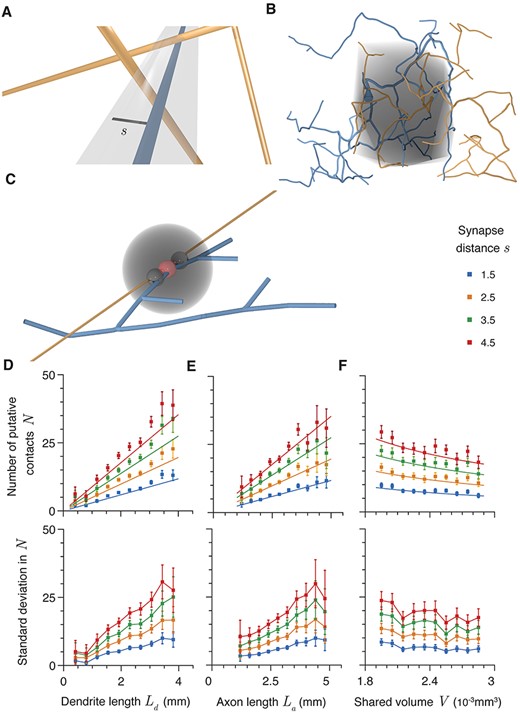
Four factors predict potential synapse number. (A) Schematic illustration of a potential contact between axonal (orange) and dendritic (blue) segments. The gray region is the cylinder of radius |$s$| (black line) within which potential contacts can form. (B) Shared volume of an example axon (orange) and dendrite (blue). The axo-dendritic overlap is shown in gray. (C) Schematic of region excluded from synapse formation (gray) caused by formation of a potential contact (red). The two black potential contacts are excluded. (D) Expected potential contact number |$N$| as a function of |${L}_{\mathrm{d}}$|, dendritic length within the axo-dendritic length. |${L}_{\mathrm{a}}$|= 3 mm and |$V$| = 2.4 |$\times{10}^{-3}$| mm3. (E) Expected potential contact number |$N$| as a function of axonal length within the axo-dendritic length. |${L}_{\mathrm{d}}$| = 2.4 mm and |$V$| = 2.4 |$\times{10}^{-3}$| mm3. (F) Expected potential contact number |$N$| as a function of the volume of the axo-dendritic overlap. |${L}_{\mathrm{d}}$| = 2.4 mm and |${L}_{\mathrm{a}}$| = 3 mm. Different colors show different maximum synapse length |$s$|. Error bars show standard error.
Defining the Axo-Dendritic Overlap
To define the boundary of the axo-dendritic overlap (Fig. 1A), the following procedure was used. The boundaries of the axonal and dendritic arbors were computed using the Trees Toolbox boundary_tree function (Cuntz et al. 2010; Bird and Cuntz 2019). Both arbors were resampled to a resolution of 1 μm using the resample_tree function. The set of axonal nodes lying within the dendritic boundary and the set of dendritic nodes lying within the axonal boundary were selected. A boundary was constructed around this set of points using the mean convexities of the two neurite arbors (see below).
Boundaries and Convexities
Boundaries are constructed using α-shapes (Edelsbrunner et al. 2006). An α-shape is a generalization of the convex hull of a point set, whereby a boundary is a set of simplices (triangles in 3D space) constructed by placing balls of radius 1/α over the point set, so that all points are contained within the ball and the vertices of the bounding simplex lie on the surface of the ball. To enable this construction, α must lie between 0 and some small positive value (the generalization to negative values is not necessary here), but small changes in α do not necessarily lead to distinct α-shapes. An α-spectrum is constructed as the set of α-intervals, which define distinct boundaries and a parameter known as the shrink factor defines the proportion of the way through this spectrum that an α value is chosen. In practice, this procedure is implemented through the MATLAB boundary function. The shrink factor is taken as one minus the convexity of a tree (Bird and Cuntz 2019).
To define the convexity of a tree, we take the set of terminal neurite points and see what proportion of the direct paths between them lie entirely within the tightest boundary (a shrink factor of 1) that contains all termination points. For a convex hull, all such paths would lie within the boundary and so this measure gives the relative difference between the two extreme shrink factors. We refer to this value, between 0 and 1, as the convexity (where 1 gives an entirely convex neuron). The Trees Toolbox function convexity_tree carries out this computation (Cuntz et al. 2010; Bird and Cuntz 2019). This procedure was originally developed for dendrites, but the extension to axonal domains here makes it potentially more likely that a terminal point will be closer in Euclidean distance to the soma than much of the intervening neurite. In this case, the direct path from the soma to these terminal points would pass outside of the tightest possible boundary and so reduce the convexity measure. This in turn would lead to a relatively tighter boundary being calculated as the spanning domain for such axons.
Estimation of Potential Synapses
Potential synaptic contacts are identified by the close apposition of dendrite and axon. An algorithm to do this for neurites in the Trees Toolbox format has been developed. The first step is to resample neurites into sections of a consistent length; this is taken to be 1 μm for spine-mediated synapses and 0.25 μm for shaft synapses; smaller values may be appropriate if the neurites have greater tortuosity. This is done with the existing resample_tree function. The second step is to identify the pairs of resampled axonal and dendritic sample points that are less than the maximal synapse distance s apart. This will typically lead to a large number of pairs of axonal and dendritic sample points that are very close together due to the connected structure of each neurite. It is rare to find such an arrangement in the data, as distinct synaptic contacts between a pair of neurons are typically more than a few microns apart. To recover a realistic distribution of contact locations and numbers, a greedy deletion step is applied. The closest pair of axonal and dendritic sample points are chosen as a synaptic contact. Then, all potential contacts where the axonal sample point is within a 3 μm distance of the axonal sample point in the existing contact and the dendritic sample point is within a 3 μm distance of the dendritic sample point in the existing contact are deleted. The closest remaining pair of axonal and dendritic sample points is chosen as a second synaptic contact and the deletion step is repeated until all inappropriate contacts are removed (Table 1).
Table summarizing symbols and terms
| Symbol | Interpretation |
|---|---|
| |${L}_{\mathrm{a}}$| | Axon length within overlapping region |
| |${L}_{\mathrm{d}}$| | Dendrite length within overlapping region |
| |$M$| | Number of dendritic compartments |
| |$n$| | Counted (numerical) number of potential contacts |
| |$N$| | Estimated (analytical) number of potential contacts |
| |${N}_{\mathrm{Complete}}$| | Number of potential synaptic contacts to innervate all dendritic compartments |
| |${p}_{\mathrm{c}}$| | Probability that a pair of cells are connected (second subscript denotes distribution model) |
| |$s$| | Distance at which a synapse can form (sum of neurite radii and, for spiny dendrites, spine length) |
| |$V$| | Volume of axo-dendritic overlap |
| |${\mu}_{M,n}$| | Expected number of dendritic compartments (out of |$M$|) innervated by |$n$| synaptic contacts |
Derivation of Analytical Estimate
As the segments are assumed to be distributed isotropically, the expected value of |$\sin \big(\theta \big)$|is |$\raisebox{1ex}{$\pi $}\!\big/ \!\raisebox{-1ex}{$4$}\big.$| and this leads directly to equation (15).
Dimensions of Dendritic Domains
The three additional domains in Figure 2A are chosen to match the volume of the cube with sides of 200 μm. Therefore, the sphere has radius 200/(4π/3)1/3 ≈ 143.30 μm and the soma is located in the center. The cylinder is chosen to have the same height and cross-sectional diameter, both are 200/(2π)1/3 ≈ 216.77 μm, again the soma is positioned in the center. The cone is chosen to have equal height and terminal diameter, both are 400/(2π/3)1/3 ≈ 312.64 μm; in this case, the soma is located at the point of the cone. It should be noted that the relationship between the volume spanned by a dendrite and the volume in which target points are distributed are not the same; the former will be bounded above by the latter as the number of target points approaches infinity (Ripley and Rasson 1977). The volume bounded by a generalized MST within a given target domain depends on the shape of that domain, the balancing factor, and the soma location. Supplementary Figure 2A shows the relationship between dendrite length and volume in the different domains.
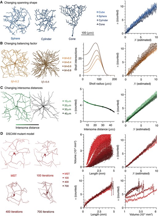
Other factors do not influence number of potential anatomical contacts. (A) Left: Example morphologies of neurites grown in different domains; from left to right, sphere, cylinder, and cone. Right: counted potential contact number as a function of estimated potential contact number for different neurite domains. (B) Left: Example morphologies generated with different balancing factors; left bf = 0.2 and right bf = 0.8. Scale bar as above. Center: Mean Sholl intersection profiles for neurons with different balancing factors. Right: Counted potential contact number as a function of estimated potential contact number for different balancing factors. (C) Left: Schematic of intersoma distance. The scale bar shows the shading of cells at different intersoma distances. Center: Mean expected numbers of contacts as a function of intersoma distance. Right: counted potential contact number as a function of estimated potential contact number for different intersoma distances. (D) Left: Example morphologies with different numbers of iterations of the DSCAM null algorithm: 0 (generalized MST), 100, 400, and 700. Center top: Volume spanned by a dendrite as a function of length for different numbers of iterations of the DSCAM null algorithm. Right top: counted potential contact number as a function of estimated potential contact number for different numbers of iterations of the DSCAM null algorithm. Center bottom: Expected number of potential contacts as a function of dendrite length. Right bottom: Expected number of potential contacts as a function of dendrite spanning volume. In all cases, error bars show standard error.
DSCAM Null Model
DSCAM null mutants have unusually clustered dendrites (Schmucker et al. 2000; Soba et al. 2007) due to the loss of transmembrane proteins that allow self-avoidance in neurites from the same cell. Dendrites with this mutation do not fill space efficiently and are not well-reproduced by the standard generalized MST model of Cuntz et al. (2010). To implement an algorithm to produce realistic synthetic dendrites, the following iterative procedure was defined:
A node |$a$| on the tree is uniformly randomly chosen.
The closest node |$b$| that is not directly connected to the first node |$a$| and is more than 2 μm away from it is identified.
The first node |$a$| is moved 10% closer to node |$b$|.
Steps 1–3 are iterated |$K$| times.
This algorithm produces dendrites with clustered branches that resemble those of DSCAM null mutants. The restriction of a minimal 2 μm distance in step 2 is necessary to prevent branches becoming “paired” and merging together, so that additional steps of 10% of the distance between them do not alter the geometry of the tree. It should also be noted that this algorithm is best applied directly to the output of the existing Trees Toolbox MST_tree function without any resampling. Increasing the number of steps |$K$| qualitatively changes the relationship between dendrite length and the volume spanned (Fig. 2D). For the DSCAM null synthetic dendrites in Figure 2, |$K$| = 100, 400, and 700.
Reconstructed Morphologies
We retrieved 75 neurons from NeuroMorpho.org (Ascoli et al. 2007) to apply our algorithm to reconstruction data. The rat barrel cortex neurons were originally obtained by (Marx et al. 2017). The data set included five different neuron types (pyramidal-like, multipolar, horizontal, tangential, and inverted) from layer 6b (N = 49) and SP (N = 26). This dataset was used as the cells were reconstructed for morphological classification from defined regions of the brain. Axons and dendrites were up to 20 and 12 mm in length, respectively. The reconstructions were preprocessed in the following way: first they were resampled to 1 μm line pieces. To separate dendrites and axons, all nodes that were not labeled as axon were deleted and the remaining nodes saved as a dendrite. The axons were obtained in the same way, but with soma and dendrite removed. The volumes and cable lengths differed widely between the reconstructions (Supplementary Fig. 3). Then dendrites and axons were randomly paired and the axon was shifted random amounts between 0 to 100 μm in the X-, Y-, Z-directions and rotated uniformly randomly. A resulting example pair of axon and dendrite can be seen in Figure 3A. The number of estimated |$N$| and counted (by directly searching for close appositions) |$n$| potential synaptic contacts were calculated for 10 000 of these combinations.
![Predictions for reconstructed morphologies. (A) Example of dendritic (blue) and axonal (orange) morphologies at an arbitrary displacement and orientation (see Methods, Marx et al. 2017). (B) Mean counted versus estimated potential contact number (blue markers and error bars). Equality is given by the black line. Error bars show standard error. Random pairs of reconstructed axonal and dendritic trees were placed at random intersoma distances and orientations (as described in Methods) and the number of potential anatomical contacts $n$ found directly. (C) Probability distribution of potential contact numbers for each integer interval of estimated potential contact number. Distributions are normalized for each estimated interval and square sizes scale linearly with the occurrence of each probability in the grid. (D) Variance in counted versus estimated mean potential contact number (blue markers and error bars). The Poisson model variance is shown by the solid red line and the best fit by the solid black line with the 95% confidence interval in gray (coefficients are 2.937 [2.8, 3.146]). The dashed blue line shows the Pólya model with parameters fitted to the connection probability. Error bars show standard error. (E) Connection probability as a function of estimated potential contact number. The fits from the Poisson, Pólya, and negative hypergeometric models are shown by the red, blue, and green lines, respectively. The fit is shown by the solid black line and gray shaded region. (F) Confidence intervals (25, 50, 75, and 95%) for values of $n$ as a function of $N$ under the negative hypergeometric model (eq. 8). In all panels, maximum synapse distance $s$ = 2.5 μm.](https://oup.silverchair-cdn.com/oup/backfile/Content_public/Journal/cercor/31/2/10.1093_cercor_bhaa271/2/m_bhaa271f3.jpeg?Expires=1749253865&Signature=FTbCVRVC62UD0LJSvnMoGkLMT6qQSqW42OGJIx2CELQxogzgA~D1XpND~TLEvCsB6UM0F8Z1uMjv7pXEo9t8XEVaylZadWzr1OEmfm6mvtFzyDcEFQVe2u1HcSW~aAn4wXWiZuKgH-x9GkaXSN2xQcmhtFlfJiwCjnCbFwU6Lp7gSQSRmuATQWV3ueqDTxJRxLyZp0vzWk-yeJD8rBQ9xWzXLo8EmaDDim9k44Yq7OT-FDWqQzJ3zwzkBtpihcwm6WdSV3glCnv9lPT1xT99cVntiDwu23g1zW011DlKXGNWHuCu8~Qy6pTjvUQka0ko2WCzI~VIU5FiAueaCp22VA__&Key-Pair-Id=APKAIE5G5CRDK6RD3PGA)
Predictions for reconstructed morphologies. (A) Example of dendritic (blue) and axonal (orange) morphologies at an arbitrary displacement and orientation (see Methods, Marx et al. 2017). (B) Mean counted versus estimated potential contact number (blue markers and error bars). Equality is given by the black line. Error bars show standard error. Random pairs of reconstructed axonal and dendritic trees were placed at random intersoma distances and orientations (as described in Methods) and the number of potential anatomical contacts |$n$| found directly. (C) Probability distribution of potential contact numbers for each integer interval of estimated potential contact number. Distributions are normalized for each estimated interval and square sizes scale linearly with the occurrence of each probability in the grid. (D) Variance in counted versus estimated mean potential contact number (blue markers and error bars). The Poisson model variance is shown by the solid red line and the best fit by the solid black line with the 95% confidence interval in gray (coefficients are 2.937 [2.8, 3.146]). The dashed blue line shows the Pólya model with parameters fitted to the connection probability. Error bars show standard error. (E) Connection probability as a function of estimated potential contact number. The fits from the Poisson, Pólya, and negative hypergeometric models are shown by the red, blue, and green lines, respectively. The fit is shown by the solid black line and gray shaded region. (F) Confidence intervals (25, 50, 75, and 95%) for values of |$n$| as a function of |$N$| under the negative hypergeometric model (eq. 8). In all panels, maximum synapse distance |$s$| = 2.5 μm.
Distribution of |$n$|
Plotting these values with parameters fitted to the measured mean and variance (in the case of the Pólya distribution) shows a poor match to the measured skewness (blue and red lines in Supplementary Fig. 3C), particularly for smaller values of |$N$|.
The interpretation of the parameters is typically that n counts the number of Bernoulli successes before |$\rho$| failures occur; initially the probability of success is |$K/\Delta$|, but each success decreases (and each failure increases) the subsequent success probability. The parameters therefore obey |$K\le \Delta$| and |$\rho \le \Delta -K$|. There is no closed-form expression for the skewness so we obtain it numerically (see below).
Fitting the three central moments, |${\mu}_h$|, |${\sigma}_h^2$|, and |${\gamma}_h$|, as well as |${p}_{c,h}$| to the data for each value of |$N$| gives the curves in Supplementary Figure 3D. The mean is fitted exactly and the sum of the relative differences of the other three statistics from their true values is minimized using the Matlab fmincon function. The negative hypergeometric distribution is a good fit for the observed distributions of |$n$| for small values of |$N$|. Supplementary Figure 3G,H show the best fits of the Poisson, Pólya, and negative hypergeometric distributions to the observed distributions of |$n$| for |$N$| = 2, and 5.
This approaches zero for |$N\approx 10$| before growing; using the more complex equation (8) instead of equation (4) has little additional utility above this value. The confidence intervals in Table 3 are therefore calculated using the most appropriate distribution.
Supplementary Figure 3I plots the distributions of |$n$| for each integer value of |$N$|under the negative hypergeometric model.
Numerical Evaluation of Equation (8) and Estimation of Skewness |${\gamma}_h$|
Akaike Information Criterion
Reconstructed Microcircuits
We retrieved 323 neurons from NeuroMorpho.org (Ascoli et al. 2007) to apply our algorithm to reconstruction data in context. The mouse visual cortex neurons were originally obtained by Jiang et al. (2015). Our dataset contained many fewer morphologies than those reported in the original paper, but comprised the full set of publicly available complete reconstructions from a slice with at least one other cell at the time of writing. It should be noted that slices with greater densities of axon pose more challenges for reconstruction. The data set included 16 different neuron types (see Table 3) from cortical layers I, II/II, and V. Cell-type labels follow directly from the labeling in the initial paper. The abbreviations used in Figure 4 and Table 3 are as follows: SBC-like, single-bouquet cell like; eNGC, extended neurogliaform cell; L23MC, layer 2/3 Martinotti cell; L23NGC, layer 2/3 neurogliaform; BTC, bitufted cell; BPC, bipolar cell; DBC, double-bouquet cell; L23BC, layer 2/3 basket cell; ChC, chandelier cell; L23Pyr, layer 2/3 pyramidal cell; L5MC, layer 5 Martinotti cell; L5NGC, layer 5 neurogliaform cell; L5BC, layer 5 basket cell; HEC, horizontally extended cell; DC, deep-projecting cell; and L5Pyr, layer 5 pyramidal cell. Dendrites and axons were up to 7.5 and 70 mm in length, respectively (Supplementary Fig. 4A,B).
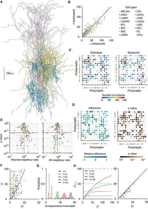
Excess potential connections in a reconstructed microcircuit. (A) Example of seven cell types reconstructed from the same slice (Jiang et al. 2015). Cells are, using the definitions in Jiang et al. (2015), L2/3 bitufted cell (2 examples), L2 Martinotti (2 examples), L2/3 chandelier (2 examples), and L2/3 bipolar (1 example). Diameters are increased by 1 μm to increase visibility and morphologies are colored by cell class (see below). (B) Measured potential connectivity as a function of estimated potential connectivity for the microcircuit data. Colors correspond to postsynaptic cell type (see legend). Maximum synapse distance varies by cell types (see Supplementary Fig. 4G). (C) Predicted (left), measured (right) cell-type specific connectivity. The horizontal axis shows the pre- and the vertical axis the post-synaptic cell types and contact numbers are per connected pair. Square sizes scale linearly with the occurrence of each connectivity in the grid. Maximum synapse distance |$s$|= 1 μm for inhibitory–inhibitory shaft synapses, |$s$|= 3 μm for other (potentially spine) synapses (Supplementary Fig. 4G). (D) Left: Relative difference of predicted from measured cell-type specific connectivities. Blue squares show where the predicted number |$n$| is greater than the expected number |$N$| and greens the converse. Square sizes scale linearly with the occurrence of the absolute value of each difference in the grid. Right: |$P$|-value of each cell-type specific measured number |$n$| of contacts occurring for each estimated number |$N$| (eqs 4 and 8). Square sizes scale linearly with the occurrence of the logarithm (base 10) of each |$P$|-value in the grid. (E) Nearest- (left) and all- (right) neighbor ratios plotted against the two-sided |$P$|-value for each cell pair. The horizontal lines show |$P$|= 0.05 and the vertical lines a ratio of 1. (F) Number of afferent contacts |$N$| as a function of the number of dendritic compartments |$M$| that could be innervated in the axo-dendritic overlap. Colors indicate dendrite type; circles correspond to the branch estimate of |$M$| and diamonds to the electrotonic estimate. The black line shows the expected number of contacts necessary to innervate every compartment (eq. 19). (G) Examples of the distributions of distinct compartments (out of 50) innervated by |$N$| = 5, 10, 25, 50, and 100 contacts (eq. 20). (H) Left: Expected number |${\mu}_{n,M}$| of distinct compartments innervated as a function of the number of contacts |$N$| for different numbers of compartments |$M$| = 10, 25, 50, and 100 (eq. 21). Solid lines show |${\mu}_{n,M}$| and dashed lines show |$M$|, the maximum possible number in each case. Right: Expected number of innervated compartments |${\mu}_{n,M}$| as a function of the number of dendritic compartments |$M$| that could be innervated in the axo-dendritic overlap (eq. 21). Colors indicate dendrite type; circles correspond to the branch estimate of |$M$| and diamonds to the electrotonic estimate. The black line shows |$M$|, the maximum number of compartments that could be innervated in each case.
The total number of neuron pairs (where pairs are imaged from the same slice) was 434, of which 233 had more than one potential contact. The reconstructions were preprocessed in the following way: first they were resampled to 0.25 μm pieces. To separate dendrites and axons, all nodes that were not labeled as axon were deleted and the remaining nodes saved as a dendrite. The axons were obtained in the same way, but with soma and dendrite removed. The volumes and cable lengths differed widely between the reconstructions (Supplementary Fig. 4A,B).
Nearest- and All-Neighbor Ratios
To establish the spatial distribution of potential contacts within the shared volume, we considered both the nearest- (NNR) and all-neighbor ratios (ANR) (Chandrashekhar 1943). The NNR quantifies the pairwise spatial correlation of points in space, whereas the ANR seeks to capture higher order correlation structure. The NNR of a set of points bounded by a given volume is defined as the mean ratio of nearest-neighbor distances to that of all possible sets of uniformly distributed points with that same space. The ANR in contrast is the mean distance of each point to the centroid of all other points in the same space. A NNR of close to one implies that points are distributed uniformly in space, whereas an ANR of one implies that at larger scales points are uniformly distributed. For each overlapping volume with |$n$| potential contacts, we generated 106 sets of |$n$|uniformly randomly distributed points to calculate the mean nearest- and all-neighbor distances. This also allowed the |$P$|-values to be computed from the proportion of random point sets that have a more extreme ratio in a given volume than the measured synaptic sites. For our data, the NNR and ANR are highly correlated (Supplementary Fig. 4C), suggesting that the higher order correlation structure is caught by the pairwise, local measure.
The neighbor ratios can often be applied in a biased manner, particularly when the boundary within which the points are to be distributed is defined by the set of points themselves (Ripley and Rasson 1977; Anton-Sanchez et al. 2018). Our application, with the boundary defined by the overlapping neurite arbors, rather than strictly the synaptic locations should be relatively free of this bias. To check whether this is indeed the case, we examined whether the volumes spanned by the boundary around the potential contacts differed systematically from the boundary around all uniform random point sets with the same number of members. Supplementary Figure 4D shows that this is not the case.
Dendritic Compartments
The passive electrotonic properties of each interneuron type were estimated from the somatic input resistance values reported in Jiang et al. (2015, see Supplementary Tables 1 and 2) and those of the pyramidal cells from the values reported by Guan et al. (2015, Fig. 2). There will always be a continuum of pairs of values of axial resistivity |${r}_a$| and membrane conductivity |${g}_m$| that lead to a given somatic input resistance for a given morphology; different pairs will also typically lead to slightly different electrotonic response properties elsewhere in neurons with tapering dendrites due to the distinct contributions of |${r}_a$| and |${g}_m$| to the local electrotonic length constant (Goldstein and Rall 1974; Bird and Cuntz 2016). We therefore restricted the allowed values to a physiological range, with axial resistivity between 50 and 200 |$\Omega$| cm and membrane conductivity allowed to vary between 0 and 10−3 Scm−2. The MATLAB patternsearch optimization function was used to minimize the difference between the mean somatic input resistance for each class of morphologies and that reported experimentally. The starting values were of |${r}_a=$|100 |$\Omega$|cm and |${g}_m=5\times$|10−5 S cm−2 and the optimization was stopped once the difference between means was below the standard error quoted in the above papers. We preferred this method to more complex compartmental modeling as the spiking properties recorded experimentally are not relevant to our study and building accurate subthreshold models would require additional data on dendritic currents. In practice, the axial resistivities remained at their initial value in all cases. The somatic input resistances reported by Jiang et al. (2015) and Guan et al. (2015) and the resultant membrane conductivities estimated by our algorithm are tabulated in Supplementary Table 1. The membrane conductivities derived in this way are higher than is sometimes reported for mouse cortical neurons in detailed electrophysiological studies, but fit the reported somatic input resistance and are consistent with the relatively fast membrane time constants also reported (Gentet et al. 2000).
The electrotonic signature, the set of transfer resistances from each node to all other nodes, was computed using the existing Trees Toolbox function sse_tree. The compartmentalization was defined by assigning a threshold value, in this case 0.13995 to match that originally used in Cuntz et al. (2010), and finding the regions of the tree within which voltages do not attenuate below this proportion of the maximum input resistance. Different thresholds lead to different numbers of compartments in a given dendrite (Supplementary Fig. 4F).
Compartments Containing a Synapse
The expected number of synaptic contacts necessary to innervate |$M$| dendritic compartments |${N}_{\mathrm{Complete}}$| in equation (19) is given by the solution to a standard problem in probability: the coupon collector’s problem (Blom 1993). The standard statement of (the simplest case of) this problem is that given a set containing elements distributed equally among |$k$| different classes, how many draws (independent and with replacement) are expected to be necessary until at least one element from each set has been drawn. This is equivalent to the problem of distributing contacts between dendritic compartments.
Reconstruction Data to Demonstrate the Predictions
We retrieved 126 mouse and 112 human cortical neuron reconstructions from the Allen Brain Institute (Allen Brain Institute 2015). Morphologies were chosen if they were marked as having a full dendrite and at least 200 μm of axon. Our dataset comprised the full set of publicly available reconstructions satisfying these criteria at the time of writing. The data set included numerous different cell types. For the mouse cells, axons and dendrites were up to 40 and 6 mm, respectively, although the majority of axons were under 25 mm. For the human cells, axons and dendrites were up to 50 and 18 mm, respectively. The reconstructions were preprocessed in the following way: first they were resampled to 1 μm pieces. To separate dendrites and axons, all nodes that were not labeled as axon were deleted and the remaining nodes saved as a dendrite. The axons were obtained in the same way, but with soma and dendrite removed. The volumes and cable lengths differed widely between the reconstructions (Supplementary Fig. 5, left hand panels). The cortical depths were recorded in the original dataset (Supplementary Fig. 5 for densities of neurite and somata with cortical depth). To generate the data for Figure 5, random pairs of axon and dendrite were chosen and displaced randomly uniformly by up to 125 μm in either direction in the plane parallel to both the slicing direction and cortical surface and by up to 25 μm in either direction in the plane perpendicular to the slicing direction and parallel to the cortical surface. Depth measurements are assumed reliable, but we introduce a small amount of jitter by displacing the depth by a normally distributed amount with mean 0 μm and standard deviation (SD) 10 μm. As these deviations are small compared with the range of possible cortical depths (Supplementary Fig. 5, right hand panels), much of the intersoma distance in Figure 5 comes from the layered structure of the cortex (Table 2).
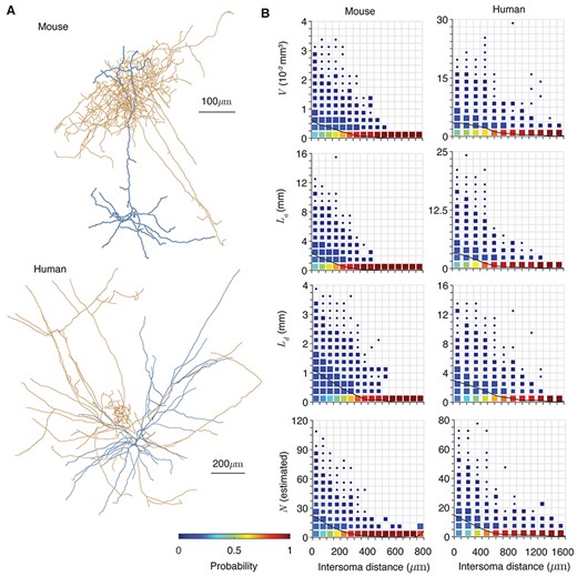
Applying the prediction of potential connectivity. (A) Example morphologies of axonal (orange) and dendritic (blue) trees from mouse (top) and human (bottom) cortex (Allen Brain Institute 2015). Diameters are increased by 1 μm to increase visibility. (B) The dependencies of shared volume |$V$|, axonal length |${L}_{\mathrm{a}}$|, dendrite length |${L}_{\mathrm{d}}$|, and expected potential synapse number |$N$| on intersoma distance for mouse (left) and human (right) cells. 104 random pairs are taken in each case. Distributions are normalized for each interval of intersoma distance and square sizes scale linearly with the occurrence of each probability in the grid. Black lines show the mean of each quantity.
Table of data sources and morphologies shown in figures
| Dataset | Figures and tables | Source | Example morphologies |
|---|---|---|---|
| Rat barrel cortex 75 cells | Figure 3 (panels A–E) | Marx et al. (2017) | Figure 3A—Axon NMO_64655, Dendrite NMO_64634 |
| Mouse visual cortex 323 cells | Figure 4*, Table 3*(all panels except F) | Jiang et al. (2015) | Figure 4A—BTC NMO_61572, BTC NMO_61573, L5MC NMO_61669, ChC NMO_61626, L5MC NMO_61670, BPC NMO_61596, ChC NMO_61627 |
| Mouse cortex 126 cells | Figure 5 (all parts) | Allen Brain Institute | Figure 5A—Axon Cell ID:584236936, Dendrite Cell ID:584872371 |
| Human cortex 112 cells | Figure 5 (all parts) | Allen Brain Institute | Figure 5A—Axon Cell ID:566350399, Dendrite Cell ID:527941296 |
Note: For the first two rows NeuroMorpho accession numbers (NMOs) are stated, for the last two rows Allen Cell Types Database IDs are stated.
Results
We first introduce a simple equation (eq. 15) that accurately estimates the expected number of potential anatomical contacts between an axonal and dendritic tree. This equation depends only on four parameters, the volume of the axo-dendritic overlap, the length of axonal and dendritic cables within this region, and the maximum length at which a synaptic contact could form. We demonstrate the equation on synthetic neurons generated using a generalized minimum-spanning tree algorithm where it is possible to vary each parameter individually. We show that the predictions of this equation are robust to changes in neuronal morphology, including the shape of the spanning domain, the centripetal bias, and the distance between somata. We next apply the prediction to reconstructed axonal and dendritic trees and estimate the full distribution of the true number of potential anatomical contacts for a given expected number. This allows us to state both the probability that a neuronal pair with given morphologies are directly connected, and the confidence intervals for their true number of contacts. We apply our predictions to a dataset of cortical neurons reconstructed in context and show that their overlapping neurite lengths are typically far in excess of those necessary to reliably ensure connectivity, instead being sufficient to expect to innervate all available dendritic compartments. We finally show another application of the original equation, comparing parameters and potential connectivity between cortical neurons from different species.
Potential Synapse Number Depends on Four Parameters
The size and shape of the axo-dendritic overlap is therefore a key component of this equation and is defined as follows. Each neuronal arbor is assigned a spanning field, a connected boundary that encompasses all neuronal branches with a tightness (Edelsbrunner et al. 2006) dependent on the underlying arbor shape (see Methods and Bird and Cuntz (2019)). The part of the axonal tree that lies within the spanning field of the dendritic arbor and the part of the dendritic tree that lies within the spanning field of the axonal arbor are used to define the axo-dendritic overlap. A boundary is created around the union of these two sections of arbor with a tightness taken as the mean of those of the two full original trees. This boundary is illustrated by the gray region in Figure 1B and the volume contained within it is defined as |$V$|.
We apply our equation to estimate the number of potential contacts between generalized MSTs (Cuntz et al. 2010) that reproduce the properties of dendritic trees, where the counted number is denoted |$n$|. Axonal trees are generated with the same algorithm as dendritic trees, but with different parameters to reflect the different branching structure. The synthetic axonal trees should therefore be considered approximations to real axons with results that are verified by reconstruction data in later figures. This allows each of the parameters |${L}_a$|, |${L}_d$|, and |$V$| to be varied independently. In order to prevent an unbounded clustering of synaptic contacts whenever an axon and dendrite pass close together at a single point, we further introduce an exclusion region around each contact (illustrated by the gray sphere in Fig. 1C). The closest apposition between dendrite and axon is selected as a contact and all other appositions within a certain distance, typically 3 μm, are excluded from forming potential contacts (illustrated by the small black spheres in Fig. 1C). The closest remaining apposition is then selected and another exclusion applied. This is repeated until there are no appositions closer than |$s$| remaining. Changing the size of the exclusion region within a reasonable range (2–25 μm) does not have a large impact on the expected number of potential contacts (Supplementary Fig. 1B). The exclusion region is a conservative constraint as Schmidt et al. (2017) found that ~20% of synaptic connections in rat medial entorhinal cortex exhibited clustering, with mean intercontact distances within a cluster of 3.7 and 4.8 μm onto excitatory and inhibitory dendrites respectively. The number of synaptic contacts given by this algorithm is therefore likely to be an underestimate of the true number, but ensures that |$n$| does not depend strongly on the sampling frequency of the neurite discretization (or grows to infinity if the neurites are treated continuously). In terms of postsynaptic functionality, tightly clustered contacts are far more likely to innervate a single dendritic compartment and so provide a strong but spatially localized input that does not alter the connectivity structure at the subcellular level.
Figure 1D–F plots the number of potential synaptic contacts found numerically for synthetic neuronal arbors generated using generalized MSTs for different maximum synapse lengths |$s$| as a function of each of |${L}_a$|, |${L}_d$|, and |$V$| when the other parameters are held approximately constant. The solid lines give the predictions of equation (15) in each case and show a good match between theory and simulation for these synthetic neurites. The SDs are plotted below the mean in each case and are quite large, growing proportionally with the mean. It should be noted that the decrease in |$N$| as a function of the overlapping volume |$V$| is a slightly artificial result as it relies on constant values of |${L}_a$| and |${L}_d$|, and therefore decreasing neurite densities. Real neurons, as shown later, do not typically display this behavior, but it is nevertheless illustrative to show that equation (15) holds even in this case.
The equation is also a simplification of the detailed approaches to estimating pairwise connectivity in Hill et al. (2012), Markram et al. (2015), and Reimann et al. (2017) as well as the dendritic-density based approaches of Liley and Wright (1994), Amirikian (2005), van Pelt and van Ooyen (2013), and Aćimović (2015). By accurately modeling potential connectivity in terms of four simple parameters, this equation simply and robustly highlights the major determinants of microcircuit structure.
Other Factors do not Substantially Influence Potential Synapse Number
Neurites take a very wide array of shapes with different branching statistics and locations relative to one another (Bok 1936; Ascoli et al. 2007; Ascoli et al. 2008); although we have shown a relationship between four features of a neuronal pairing and the expected potential synapse number |$N$|, it is worthwhile to consider whether other factors implicit to the dendrites in our model may have an effect. We have therefore investigated whether three other features alter the accuracy of the prediction under equation (15). Firstly we considered whether the shape of the domain used to create the synthetic neurites has an impact. For Figure 1, the generalized MST algorithms were used to generate trees within cubes, but various other shapes such as cones, spheres, and cylinders do not affect the results (Fig. 2A). All bounding shapes were taken to have the same volume as the original cube (although there may well be systematic differences in the regions bounded by the resultant neurites, see Methods).
The balancing factor bf in the generalized MST model determines the balance between costs associated with additional neurite length and conduction delays caused by long path distances between synapses and the soma. A balancing factor of zero corresponds to a pure MST where conduction delays are ignored and in the limit of high balancing factors, all synapses are directly connected to the soma. Typically real nonplanar neurons have dendrites with balancing factors in the range 0.2–0.9 (Cuntz et al. 2010) and there is a roughly exponential relationship between increasing balancing factor and the centripetal bias as measured by the root angle distribution. The root angle distribution quantifies the angular divergence of dendritic branches from a direct path to the soma (Bird et al. 2019). For cortical Martinotti interneurons, balancing factors tend to range from 0.65 to 0.75, whereas for dentate gyrus granule cells balancing factors tend to cluster ~0.9. We typically set the balancing factors of the dendrite and axon to 0.2 and 0.7, respectively to account for the different features of these neurites (Cuntz et al. 2007; Budd et al. 2010; Teeter and Stevens 2011). The construction of axons in this way is less well established than the construction of dendrites, and we later verify our results with reconstructed data. Varying the dendritic balancing factor over the range 0.2–0.8, the majority of the range observed in reconstructed neurons, whilst keeping other features, such as bounding shape, the same does not alter the accuracy of the predictions of equation (15) (Fig. 2B). This result is particularly surprising as we have recently shown that different balancing factors lead to substantially different distributions of neurite mass within their spanning fields (Fig. 2B, center) and violates the assumption of isotropically distributed branches through its effect on the root angle distribution.
Finally, the intersoma distance does not matter as long as the cable lengths and overlapping volume are controlled for (Fig. 2C). Intersoma distances were fixed at 10, 20, 30, and 40 μm. This last point is particularly interesting, as a number of studies report a strong influence of intersoma distance on predicted connectivity (Hellwig 2000; Kalisman et al. 2003; van Pelt and van Ooyen 2013); we find that intersoma distance only matters through the negative correlation between distance and the neurite lengths within an overlapping volume. Varying the bounding shape, balancing factor, and intersoma distance together within the ranges specified above had no effect on the accuracy of the estimate (Supplementary Fig. 2D).
Clustered Dendrites do not Cause a Loss of Potential Connectivity
The above results are for dendrites with the properties of relative space-filling and spatial uniformity particular to trees that minimize metabolic costs (Cuntz et al. 2007; Wen et al. 2009; Bird and Cuntz 2019). The results of equation (15) still hold, however, when these properties are violated. Inspired by invertebrate neurons with a DSCAM null mutation (Schmucker et al. 2000), which reduces the self-avoidant tendency of neurites and leads to pathologically clustered dendrites (Soba et al. 2007), we introduce an algorithm that modifies the existing MST model to produce artificial neurites that have similar properties. The new algorithm, described in Methods, iteratively randomly selects branches of the neurite and moves them 10% closer to the closest neighboring branch. Iterating this process produces progressively more clustered morphologies (Fig. 2D, left).
Increasing the number of iterations changes the relationship between length and volume as dendrites become more densely clustered (Fig. 2D, center top). However, when applied to such arbors, the predictions of equation (15) still hold (Fig. 2D, right top). This means that the potential connectivity of neurites that do not effectively fill space remains predictable from equation (15); clustering of synthetic dendrites does not cause loss of function through lost connectivity beyond that predicted by changes in dendrite length and spanning field (Mychasiuk et al. 2012). This is a slightly counterintuitive finding as Wen et al. (2009) found that normal dendritic branching statistics are in line with those that maximize the connectivity repertoire of afferent connections. The new algorithm causes a greater density of dendrite within its spanning field and so such trees have a relatively high number of potential contacts within a given spanning volume (Fig. 2D, center bottom). However, this is balanced by the reduced amount of axon that typically intersects the dendritic spanning field and so the clustering has no effect on the relationship between the length of the dendritic tree and the expected number of contacts it receives (Fig. 2D, right bottom).
Synapse Estimation for Reconstructed Morphologies
Our model produces accurate estimates of potential synaptic contact number for the generalized MST models that accurately simulate real neurites, but also applies directly to neural reconstructions. To demonstrate this, we consider a dataset of 75 reconstructions from the rat barrel cortex and developmental subplate by Marx et al. (2017). These neurons were reconstructed for morphological clustering and have recorded axons up to 20 mm long (Supplementary Fig. 3A). When neurons are randomly paired with random offsets in their somata and orientation (see Methods and Fig. 3A), equation (15) correctly predicts the number of potential axo-dendritic synaptic contacts (Fig. 3B). The mean squared error (MSE) is 0.628. The distribution of counted values of |$n$| for each expected value |$N$| is shown by the heatmap in Figure 3C.
It is interesting to note the variability in these results. Figure 1D–F shows the variance in the counted value of |$n$| as a function of the underlying parameters and it typically takes large values. Similarly, Figure 3D shows the distribution of counted values of |$n$| for each estimated integer value of |$N$|. Both illustrate the large variation in possible true numbers of potential contacts for a given set of parameters |${L}_a$|, |${L}_d$|, and |$V$|. The wide variability here means that equation (15) is unlikely to be perfectly accurate when applied to a single axo-dendritic pair, but is a true estimate of the expected number of potential contacts, between a large number of pairs, using relatively simple parameters.
Connection Probability |${p}_c$| and the Distribution of |$n$|
The Pólya distribution (eq. 4) modifies the Poisson distribution to allow the mean and variance to differ and can be used to describe correlated occurrences (Blom,1993). The variance in |$n$| grows faster than |$N$| and is well-described by a function of the form |$\operatorname{var}(n)= aN+{N}^b$| where the parameters are (with 95% confidence intervals) a = 2.944 (2.769, 3.119) and b = −0.124 (−0.246, −0.001). This is plotted as the solid black line and shaded gray area in Figure 3D (MSE 12.099). The second term |${N}^b$| is necessary to capture the initial growth in the variance for small values of |$N$| that is particularly apparent when plotting the Fano factor |$\operatorname{var}(n)/N$| in Supplementary Figure 3B. It should be noted that the variance in |$n$| as a function of |$N$| is fundamentally different to the variances in |$n$| as functions of |${L}_a$|, |${L}_d$|, and |$V$| shown in Figure 1 The estimates of each value of |$N$| come from a wide variety of possible combinations of the underlying parameters that obey equation (15); the resultant variance in |$n$| therefore has a complex dependence on the underlying factors, weighted by their joint likelihood of occurrence, that is best described empirically.
When comparing models of different levels of complexity, the Akaike Information Criterion (Akaike 1974) provides an estimate of the relative information lost by encoding data with a given equation, and therefore the quality of that model (see Methods). The criteria can be calculated for the three distributions on each interval of estimated |$N$| in Figure 3. The criteria of the Poisson, Pólya, and negative hypergeometric distributions when |$0.8\le N<1$| are 957.33, 819.26, and − 445.11, respectively. This is very strong evidence that the negative hypergeometric model should be used in this range of |$N$|. For |$4.8\le N<5$|, the criteria give 996.39, 800.75, and 794.24, implying that the probability that the Pólya model is a better representation of the data here than the negative hypergeometric model is only 0.039. By |$9.8\le N<10$|, however, the criteria are 331.42, 280.47, and 282.26, indicating that the three parameter negative hypergeometric model does not provide a sufficiently better fit to the data to justify its additional parameter over the Pólya model. For larger values of |$N$| (|$\gtrsim 10$|), the Pólya distribution should be the preferred model as it has fewer parameters, is more analytically tractable, and has well-defined moments. For smaller values of |$N$|, the negative hypergeometric model is a better fit to the connection probability.
Synapse Estimation for Reconstructed Microcircuits
In the previous sections, we considered the number of potential contacts between reconstructed morphologies with random somatic locations. This verified the predictions of the generalized MST model for real axons and dendrites, but left open the question of how the specific arrangement of axonal and dendritic spanning fields within cortical circuits can lead to certain connectivity patterns. Jiang et al. (2015) produced a dataset of reconstructions from the visual cortex of adult mice, and in particular often reconstructed multiple cells from the same slice (Fig. 4A), allowing equation (15) to be tested on a large set of cells in context with one another. Here, the maximum synapse distance |$s$| varies between 1 μm for synapses between inhibitory neurons which are assumed to lie only on the dendritic shaft and 3 μm for those which could potentially be mediated by a spine (Villa et al. 2016; Sancho and Bloodgood 2018). Such assumptions are potentially artificial as some inhibitory neurons, such as chandelier cells, do not form dendritic synapses at all; it is nevertheless interesting to see whether this impacts their actual axonal branching patterns as shown by the potential connectivity.
The predictions hold very well, allowing accurate estimation of both overall (Fig. 4B) and cell-type specific (using the classes described by Jiang et al. (2015), Fig. 4C) potential connectivity. It should be noted, however, that there are relatively few cells per class (typically between 15 and 25), and that the morphological classification used by Jiang et al. (2015) identified fewer distinct classes than more recent transcriptomic classification (Tasic et al. 2018). Despite broad agreement, there do appear to be some differences between the two measures when the relative differences from the counted number |$n$| are plotted (Fig. 4D). For example the measured potential connectivity of L2/3 neurogliaform cells to bitufted cells appears significantly higher than that predicted using the distribution of |$n$| for a given value of |$N$| derived above. This is potentially interesting, as the neurogliaform cells were observed by Jiang et al. (2015) to induce distinct postsynaptic potentials reminiscent of volume transmission (Chittajallu et al. 2013) and may obey distinct local axon branching statistics. In this case, functional connectivity would not be entirely dependent on potential contacts between axon and dendrite as neurotransmitters would have a more spatially diffuse action alongside directed functional contacts. Indeed, the three types of neurogliaform cell do have relatively low |$P$|-values for a number of postsynaptic neuron types. However, with a dataset of this size, such differences could also arise as an artifact of testing pairwise potential connectivity between multiple cell classes. Applying a multiple-testing correction (Bonferroni 1936), gives no cell-type specific differences between |$n$| and |$N$| that are significant at the |$P=0.05$| level. More data would therefore be necessary to resolve the local structure of these axons and quantify important differences in resultant potential connectivity.
Potential Contact Numbers Often Exceed Those Necessary for Reliable Connectivity
The numbers of potential contacts from both equation (15) and direct measurements are often very high in this dataset. Experimental studies find many fewer functional contacts, often an order of magnitude lower, between cell pairs (Markram et al. 1997; Kasthuri et al. 2015; Lee et al. 2016). An initial hypothesis would be that very high numbers of potential contacts are necessary to increase the probability of having at least one potential connection in order to allow a microcircuit to function. Under the model of equation (17), we estimate that the probability that the cell pair with the greatest number of potential synapses, an elongated (L1) neurogliaform to L2/3 neurogliaform cell, would be disconnected given their neurite lengths within the overlapping region is or less than one in 3 million. If the axon length within the overlapping volume were to half, the probability of no connection would still be one in 30 000. For the 10th most potentially connected cell pair, a pair of L2/3 double bouquet cells, the probabilities decreases from one in 200 000 to one in 5000. These probabilities are not that low given the number of cells within a cortical column, but do suggest that the metabolic cost to reliably establish single connections is far below that typically paid by these cells. Stepanyants et al. (2008) estimated that potential connectivity within local circuits in the cat visual cortex is all-to-all, but the estimates of potential contacts here go beyond those necessary to achieve this. It should also be noted that slicing artifacts, by removing neurite outside of the slice, will tend to introduce both upwards and downwards biases in the numbers of potential contacts that cannot be readily addressed by this data (Jiang et al. 2016); in intact cortex, the potential connectivity will be affected by appositions outside of the slice, as well as sections of axons that leave the slice before returning to potentially innervate a different region. Our findings are in line with the very high degree of synaptic redundancy observed by Kasthuri et al. (2015) in mature mouse somatosensory cortex and Lee et al. (2016) in mature mouse visual cortex.
Potential Contacts are Well-Distributed Within the Axo-Dendritic Overlap
To determine the distribution of potential connections within the axo-dendritic overlap, and in particular whether they are more clustered or more regular than a uniform random spatial distribution (i.e., a homogeneous spatial Poisson process, see Methods), we used both the NNR and the ANR (Chandrashekhar 1943). The NNR quantifies whether the distance between a potential contact and the closest other contact is more or less than would be expected for a spatially homogeneous random process. A NNR of one implies that the potential contacts are distributed within the axo-dendritic overlap precisely as one would expect from a homogenous Poisson process, whereas a ratio of less than one implies clustered and more than one well-distributed potential contacts. The number of potential contacts varies widely between cell pairs, so |$P$|-values (see Methods) are plotted against the NNR in Figure 4E to indicate the significance of the difference from one for each cell pair.
As synaptic contacts are distributed along neurite arbors, there is potential for local spatial correlations to arise and dominate the pairwise measure given by the NNR. To determine whether the contacts display local correlation along arbors, but more general independence, we also computed the ANR: the average deviation of each potential contact from the centroid of all contacts. This measure is less sensitive to local correlation and is plotted in Figure 4E.
Both measures show that there is a spread of ratios; 35 of 233 pairs with more than one potential contact are significantly clustered and 31 are significantly regular under the NNR, with numbers of 53 and 35 for the ANR. However, there appears to be no significant and consistent clustering or regularity by either pre- or post-synaptic cell types (see Table 3 for mean nearest-neighbor values and |$P$|-values by presynaptic class for all other classes in the dataset). This lack of apparent spatial structure in potential connections between a cell pair is an interesting intermediate case. Merchán-Pérez et al. (2014) found uniform randomness in the location of all synapses within a volume of neuropil without reference to specific neurites, while synapses along a given axon or dendrite will be clearly spatially correlated. van Pelt and van Ooyen (2013) concluded that spatial correlations were the cause of the mismatch between their model of density-based mean potential contact number prediction and the connection probability and we have observed a similar effect (Fig. 3E). However, they did not directly check for spatial correlations in potential contacts and appear to use lower neurite densities than those seen in the reconstructed data here, which could enhance the impact of potential contacts sharing a branch. Of particular interest, here is that inhibitory cell types do not appear to form potential contacts in a more spatially structured way than excitatory cells (see Table 3). This is despite the fact that cortical inhibitory neurons stereotypically innervate specific regions of excitatory cells, for example basket cells tend to form perisomatic synapses and chandelier cells synapse onto the axon initial segment of excitatory neurons (Ascoli et al. 2008; Hill et al. 2012). These results suggest that such specificity could come entirely from the axonal growth region rather than individual local targeting processes.
Columns from left to right are: cell type, mean total number of dendritic compartments |$M$|, mean number of dendritic compartments |${M}_{\mathrm{Prop}}$| that lie within the axo-dendritic overlap, ratio of number of afferent synapses |$n$| to the number necessary to expect to innervate each available dendritic compartment |${N}_{\mathrm{Complete}}$| (with 95% confidence interval), and ratio of mean number of available compartments innervated |${\mu}_{M,n}$| to number of available of compartments |$M$| (with 95% confidence interval)
| Cell_type | Numbers | Efferent contacts | Afferent contacts | Compartments | ||||||
|---|---|---|---|---|---|---|---|---|---|---|
| Examples | Pairs | Nefferent | NNR | Mean p-value | Nafferent | M | MProp | |$ \frac{n}{N_{Complete}} $| | |$ \frac{{\boldsymbol{\mu}}_{\boldsymbol{n},\boldsymbol{M}}}{\boldsymbol{M}} $| | |
| Sing_Boquet_Like | 21 | 22 | 25.79 ± 7.66 | 1.04 ± 0.18 | 0.39 (0.25) | 37.43 ± 9.05 (23.39,53.54) | 22.52 ± 1.95 12.86 ± 1.92 | 11.79 ± 2.05 7.29 ± 1.68 | 2.45 ± 0.62 (1.1,3.91) 8.85 ± 2.86 (4.49,13.99) | 0.7 ± 0.08, (0.51,0.74) 0.73 ± 0.08, (0.58,0.75) |
| Neuroglia_F | 21 | 17 | 58.05 ± 11.67 | 0.89 ± 0.11 | 0.31 (0.29) | 65.55 ± 12.65 (44.23,89.55) | 22.57 ± 1.97 14.43 ± 1.64 | 11.59 ± 1.67 6.59 ± 1.13 | 2.48 ± 0.39 (1.24,3.78) 10.88 ± 3.64 (5.96,16.58) | 0.85 ± 0.07, (0.71,0.86) 0.86 ± 0.07, (0.75,0.86) |
| LII_Martinotti | 20 | 51 | 39.88 ± 4.89 | 1.36 ± 0.12 | 0.29 (0.32) | 45.01 ± 4.79 (27.85,64.56) | 29.4 ± 2.47 15.35 ± 1.77 | 14.28 ± 1.07 6.59 ± 0.61 | 1.3 ± 0.12 (0.7,1.96) 4.79 ± 0.65 (2.66,7.11) | 0.76 ± 0.05, (0.59,0.78) 0.79 ± 0.05, (0.65,0.79) |
| LII_Neuroglia_F | 20 | 28 | 67.4 ± 11.6 | 1.12 ± 0.09 | 0.39 (0.28) | 92.54 ± 11.12 (65.97121.71) | 32.1 ± 3.11 14.8 ± 1.98 | 17.2 ± 1.6 8.74 ± 1.37 | 1.92 ± 0.23 (1.16,2.73) 27.95 ± 9.14 (19.98,36.58) | 0.86 ± 0.05, (0.75,0.88) 0.88 ± 0.05, (0.77,0.88) |
| LII_Bitufted | 20 | 50 | 54.13 ± 6.37 | 0.94 ± 0.05 | 0.39 (0.21) | 40.16 ± 5.46 (24.42,58.27) | 21.15 ± 2.41 10.65 ± 2.43 | 9.83 ± 1.12 4.84 ± 0.96 | 2.1 ± 0.27 (0.92,3.45) 16.89 ± 2.62 (8.64,26.63) | 0.84 ± 0.04, (0.61,0.86) 0.86 ± 0.04, (0.68,0.84) |
| LII_Bipolar | 20 | 54 | 43.32 ± 5.61 | 1.29 ± 0.43 | 0.3 (0.18) | 23.51 ± 4.11 (13.28,35.3) | 19.1 ± 2.43 9.75 ± 1.7 | 9.59 ± 1.28 5.08 ± 0.84 | 2.98 ± 0.52 (1.19,5.07) 11.07 ± 2.04 (5.36,17.7) | 0.69 ± 0.06, (0.44,0.71) 0.7 ± 0.06, (0.45,0.71) |
| LII_Double_Bouquet | 20 | 15 | 64.71 ± 16.36 | 1.04 ± 0.16 | 0.34 (0.22) | 63.29 ± 13.96 (43.19,85.86) | 22.7 ± 2.94 13.9 ± 1.81 | 14.2 ± 1.94 8.25 ± 1.22 | 2.57 ± 0.73 (1.52,3.7) 5.7 ± 2.13 (3.43,8.22) | 0.77 ± 0.09, (0.67,0.79) 0.78 ± 0.09, (0.69,0.74) |
| LII_Basket | 15 | 16 | 52.79 ± 13.65 | 0.82 ± 0.08 | 0.24 (0.43) | 53.17 ± 13.77 (36.21,72.75) | 23.27 ± 2.34 17.4 ± 2.03 | 14.21 ± 1.86 10.33 ± 1.35 | 1.66 ± 0.52 (1.07,2.35) 7.65 ± 5.98 (5.38,10.22) | 0.68 ± 0.08, (0.53,0.74) 0.71 ± 0.08, (0.56,0.72) |
| LII_Chandelier | 20 | 15 | 26.24 ± 8.45 | 1.09 ± 0.1 | 0.47 (0.13) | 19.47 ± 5.58 (8.76,32.35) | 18.9 ± 2.09 11 ± 2.05 | 4.65 ± 1.37 4.71 ± 1.06 | 3.4 ± 0.84 (1.24,6.08) 2.72 ± 0.5 (0.93,4.89) | 0.87 ± 0.08, (0.57,0.88) 0.85 ± 0.08, (0.57,0.88) |
| LII_Pyr | 20 | 9 | 29.38 ± 9.61 | 1.36 ± 0.33 | 0.61 (0) | 28.46 ± 9.29 (15.92,43.46) | 33.9 ± 3.1 15.95 ± 2.41 | 15.85 ± 3.98 7.77 ± 2.88 | 1.52 ± 0.66 (0.81,2.35) 21.14 ± 9.72 (12.34,31.67) | 0.72 ± 0.12, (0.5,0.76) 0.77 ± 0.12, (0.67,0.77) |
| LV_Martinotti | 21 | 42 | 33.69 ± 5 | 1.31 ± 0.08 | 0.39 (0.3) | 39.63 ± 5.09 (23.54,58.27) | 24.48 ± 2.08 11.57 ± 2.07 | 9.21 ± 0.91 3.54 ± 0.61 | 2.13 ± 0.34 (1.05,3.43) 22.02 ± 4 (12.21,33.48) | 0.83 ± 0.05, (0.64,0.86) 0.86 ± 0.05, (0.71,0.87) |
| LV_Neuroglia_F | 21 | 19 | 69.24 ± 17.55 | 1.26 ± 0.15 | 0.28 (0.4) | 67.84 ± 15.58 (48.6,89.24) | 26.86 ± 2.41 17.19 ± 2.21 | 16.8 ± 1.86 10.32 ± 1.77 | 2.11 ± 0.53 (0.99,3.27) 10.18 ± 3.63 (6.76,13.96) | 0.65 ± 0.09, (0.55,0.69) 0.66 ± 0.09, (0.56,0.66) |
| LV_Basket | 21 | 36 | 50.43 ± 8.58 | 0.94 ± 0.08 | 0.28 (0.32) | 54.37 ± 8.58 (35.39,75.96) | 24.48 ± 2.43 15.52 ± 1.8 | 12.55 ± 1.45 8.25 ± 0.92 | 2.45 ± 0.34 (1.14,3.87) 7.66 ± 2.92 (4.39,11.37) | 0.85 ± 0.04, (0.61,0.93) 0.89 ± 0.04, (0.69,0.9) |
| LV_Horiz_Extend | 21 | 32 | 54.71 ± 10.06 | 1.11 ± 0.14 | 0.14 (0.41) | 56.78 ± 9.92 (38.44,77.78) | 25 ± 2.08 15.52 ± 1.85 | 11.39 ± 1.02 6.02 ± 0.71 | 1.76 ± 0.24 (1.04,2.59) 6.57 ± 1.76 (4.21,9.27) | 0.81 ± 0.05 (0.6,0.84) 0.83 ± 0.06 (0.66,0.85) |
| LV_Deep_Proj | 21 | 19 | 23.58 ± 7.87 | 1.23 ± 0.34 | 0.33 (0.29) | 36 ± 9.39 (22.58,51.58) | 24.19 ± 3.49 14.81 ± 2.07 | 12.96 ± 2.22 8.08 ± 1.7 | 1.96 ± 0.55 (0.96,3.2) 4.94 ± 1.62 (2.64,7.73) | 0.63 ± 0.09 (0.55,0.65) 0.65 ± 0.09 (0.58,0.65) |
| LV_Pyr | 21 | 9 | 42.18 ± 20.04 | 2.63 ± 0 | 0.09 (0) | 40.36 ± 20.16 (27.36,55.55) | 31.38 ± 3.67 17.29 ± 3.41 | 13.82 ± 3.36 7.45 ± 2.62 | 1.23 ± 0.5 (0.78,1.78) 17.41 ± 10.16 (10.53,25.68) | 0.55 ± 0.14 (0.44,0.6) 0.59 ± 0.15 (0.55,0.62) |
Notes: For the last four columns, the upper values come from the branch-based estimate of compartments, and the lower from the attenuation-based estimate. |$\pm$| shows the standard error over different cells of each class and confidence intervals are for the mean of each class using equations (4) and (8).
Excess Potential Connections Allow for the Innervation of Multiple Dendritic Compartments
Given that expected potential contact numbers are far in excess of that necessary to produce reliable connectivity at the cellular level, and that contacts lack apparent spatial structure, it is both informative and feasible to investigate how cortical neurite densities can implement subcellular connectivity by innervating specific or distinct dendritic compartments. Definitions of dendritic compartments vary in the literature (Mel 1993; Poirazi et al. 2003; Polsky et al. 2004; London and Häusser 2005; Branco and Häusser 2010; Cuntz et al. 2010; Behabadi et al. 2012) and certainly the electronic structure of a dendritic tree changes dynamically with network activity due to both synaptic activation and thresholded processes (Llinas 1988; Schiller et al. 2000; Gidon and Segev 2012; Ferrarese et al. 2018; Wybo et al. 2019). To investigate compartmentalization, we consider two simple descriptions of a dendritic compartment. The first is simply that each individual dendritic branch is a compartment (Branco and Häusser 2010) and the second assigns reasonable passive electrotonic properties (see Methods) to a dendrite and divides the tree into regions within which synaptic currents do not attenuate below a certain threshold (Cuntz et al. 2010). The first estimate is indicated by diamonds and the second by circles in Figure 4F,H. These are both certainly drastic simplifications of the true integrative properties of a dendrite, particularly within an active microcircuit, but provide an informative first step. To account for the fact that the axo-dendritic overlap only covers a part of the dendrite, we scale the compartment number down to match the proportion of dendrite that lies within this volume.
Figure 4H (left side) plots |${\mu}_{M,n}$| as a function of |$n$| for different values of |$M$|, highlighting the asymptotic behavior as |$n$| grows larger than |$M$|. The right-hand side of Figure 4H plots |${\mu}_{M,n}$| against |$M$| for the cells in this dataset, given the number of potential contacts they receive. Many cell pairs have sufficient potential contacts to expect to be able to innervate almost all of the available dendritic compartments. In Table 3, the ratio of |${\mu}_{M,n}$| to |$M$| is frequently above 0.75 when averaged over each cell class, meaning that three out of four available compartments could potentially receive a synaptic contact.
Applying the Prediction of Potential Connectivity
As a final demonstration of the utility of equation (15) in predicting potential connectivity, we show how the neurite lengths and shared volumes, as well as the expected number of potential synapses, vary with intersoma distance for the reconstructed cortical morphologies of mouse (Fig. 5A, top) and human (Fig. 5A, bottom) cells published by the Allen Institute for Brain Science (Allen Brain Institute 2015). These cells are not typically imaged in context, but do have the depth of the soma below the cortical surface reliably recorded, alongside the orientation within the slice (see Supplementary Fig. 5). For the demonstration in Figure 5, we randomly pair axonal and dendritic reconstructions using their recorded cortical depth and a random offset in the plane parallel to the cortical surface (see Methods). This allows an estimation of the potential connectivity between cells further apart than those imaged in context, but retaining realistic orientations and depths.
We can see a decrease in all three relevant parameters |${L}_a$|, |${L}_d$|, and |$V$| with increasing intersoma distance (Fig. 5B, top three panels), and the fact that the expected number of potential contacts depends on the product of |${L}_a$| and |${L}_d$|, over |$V$| means that this is accompanied by a decrease in |$N$| (Fig. 5B, bottom panels). These predictions give an intuition of the structural backbone to functional connectivity in cortex that can be progressively refined as more reconstructions of individual cell types appear. In terms of excess connectivity, it can also be seen that large numbers of potential contacts (|$N$| > 50) can arise when the intersoma distance is less than ~400 μm for both mouse and human neurons.
Discussion
Summary
We have demonstrated that the expected number of potential synaptic contacts between a pair of neurons is given by a simple equation (eq. 15) and depends on the volume of axo-dendritic overlap, the lengths of axon and dendrite within this region, and the maximum length of dendritic spines. Moreover, if these four factors are controlled for, the number of synapses is insensitive to domain shape, intersoma distance, centripetal bias, and morphological changes that cause clustering. These results also hold for reconstructed cortical axons and dendrites at random distances and orientations and are simply applicable to real cells. We have accurately estimated the probability distribution of the counted number of potential contacts for an expected number given by our equation. When applying our results to cells reconstructed in context, we found an excess of potential local connectivity, meaning that each pair of cells within a circuit in mature cortex could potentially be connected multiple times. The excess branching within, and overlap between, the neurite spanning fields mean that the lengths of axon and dendrite available to form connections can be surprisingly high. The potential contacts are distributed in space and, on average for each cell class, each axon could be expected to target every available dendritic compartment, whether defined by branches or by electrotonic attenuation. This suggests that such cortical microcircuits may require potential connectivity to specific dendritic compartments, rather than simply at a cellular level, and are able to achieve this.
Context
Theoretical estimates of potential synaptic connectivity between pairs of neurons have long been sought alongside experimental approaches to clarify and generalize the principles observed. It is useful to consider the other approaches taken to this problem, to demonstrate how the estimates of our equation (15) fit into the broader literature on potential connectivity.
An early analytical approach by Uttley (1955) estimated the number of close appositions of axon and dendrite by assuming random and independent neurite growth and its implications on the resultant densities of cable. Liley and Wright (1994) built on this, using a spherically symmetric simplification of dendritic density based on the Sholl intersection profile (Sholl 1953) to estimate the probabilities of given numbers of anatomical connections forming between pairs of cortical cells. Stepanyants et al. (2002) considered the relationship between potential and actual connectivity, introducing the concept of the filling fraction and modeling the number of potential contacts using the independent features of the axon and dendrite. Kalisman et al. (2005) used the detailed structure of complete reconstructions to generate more realistic cylindrically symmetric estimates of cortical neurite density and find the probability of potential synapses forming between cell pairs. Stepanyants et al. (2004) studied specific connectivity between interneurons and pyramidal cells, confirming that specificity in connections could arise from overlapping volumes of axon and dendrite even in the absence of correlations between neurite branches and finding a linear increase in potential connectivity with maximum synapse distance. Chklovskii (2004) considered the volume of connected neuronal circuits and determined the relative contributions of branched axons, dendrites, and dendritic spines to allowing physiological levels of compactness. In particular, this study estimates the expected number of afferent synapses onto a given neuron from the length of its dendrite, maximal synapse length, and the amount of axon in the surrounding tissue. Amirikian (2005) also assumed a cylindrically symmetric density of synapses (based on the dendritic density given by the Sholl intersection profile in a similar manner to Liley and Wright (1994)) and found good agreement with data for a number of cell classes, in particular correctly determining both axo-dendritic and axo-somatic synapses. Stepanyants et al. (2008) estimated potential connectivity in the cat visual cortex, finding all-to-all connectivity for cells within 200 μm. Wen et al. (2009) considered the connectivity repertoire, the number of possible patterns of synaptic contacts a given dendrite can receive. During this study, estimates of the numbers of synaptic contacts onto Purkinje and pyramidal cell basal dendrites were derived in terms of their length, maximal synapse distance, and spanning field. Hill et al. (2012) took a different approach, using full reconstructions to determine potential synaptic contacts and finding excellent agreement with the potential synapses found experimentally. van Pelt and van Ooyen (2013) directly compared the connectivity predictions from neurite density fields with those of the full arbors, finding that whilst predictions from density fields do generally match the expected number of anatomical contacts, they are unreliable estimators of both the absolute connection probability (the probability that at least one anatomical contact occurs) and the true distribution of possible contact numbers. McAssey et al. (2014) greatly expanded on the previous study, simulating the connections between 10 000 artificially constructed dendrites and relating these to those derived from the neurite density fields. Reimann et al. (2015) developed the approach of Hill et al. (2012) using observed axo-dendritic overlaps to refine the connectivity patterns, producing a simulated cortical column connectome that was explored by Markram et al. (2015). Aćimović et al. (2015) used the Gaussian description of dendritic density introduced by Teeter and Stevens (2011) to examine how changing the parameters of simplified dendrites could affect the connectivity structure of a large network.
Our approach can be seen as a broad generalization of the above studies. The estimate of equation (15) is not dependent on the local branching statistics of different neuronal types, such as those of Kalisman et al. (2003, 2005), Hill et al. (2012), and Reimann et al. (2015, 2017), nor does it rely on the density of neurite within a spanning field such as the work of Uttley (1955), Liley and Wright (1994), Amirikian (2005), van Pelt and van Ooyen (2013), McAssey et al. (2014), and Aćimović et al. (2015). The simple form of equation (15) is of the same form as the equations derived by Stepanyants et al. (2002) and Chklovskii (2004) for the total number of synapses in a volume of neural tissue; the novelty of our result is that such a simple equation can be reliably applied to individual cell pairs by using a precise definition of the axo-dendritic overlap. In addition, we have been able to further estimate the distribution of the true number of potential contacts for an expected value given by equation (15), which means that the typical variation in potential contacts between real cell pairs can be quantified.
Outlook
This study provides a simple way to verify the degree of targeting within a neuronal circuit; for a given pair of neurons, the expected number of potential synaptic contacts is predictable by our equation. When the number of close appositions is consistently different from that predicted here, particularly when it is outside our variability estimates, there is evidence of local targeting in the neurite growth processes and potential for a higher degree of hard-coding or specificity in a circuit. This could help to explain some of the controversy over the applicability of versions of Peters’ rule in different systems (Rees et al. 2017), and will become more valuable as connectome data becomes increasingly available (da Costa and Martin 2013; Helmstaedter 2013; Kasthuri et al. 2015; Lee et al. 2016; Iascone et al. 2020). A particular application could be to compensate for the loss of connectivity due to slicing and reconstruction artifacts. The Allen Brain Institute marks cuts on their connectome data (Allen Brain Institute 2015 and the Blue Brain Project simulates neurite morphologies outside of the slice (Hill et al. 2012; Reimann et al. 2015), best practice here is controversial (Barth et al. 2016; Jiang et al. 2016). The equation derived here provides a simple sanity check on the reasonableness of such corrections. In addition, with some further information about the postsynaptic cell, for example the centripetal bias and dendritic diameter taper, it should be possible to estimate the expected locations of synaptic contacts along a dendrite from relatively general principles. This is an interesting area of further study.
We would also like to highlight the importance of the location and shape of the axo-dendritic overlap. Our results suggest that this is both important for the overall connectivity estimate and sufficient to predict the potential locations of inhibitory connections that are known to be highly specific (Ascoli et al. 2008). Hill et al. (2012) found that the statistical description of neuronal morphologies in isolation failed to predict the connectivity of such interneurons, in particular chandelier cells where the interaction of axon and dendrite is assumed to provide additional growth guidance. By taking the overlapping volume relative to the two cells in context, this factor is already accounted for and a random distribution of neurite within this volume is sufficient to predict connectivity. This contributes to the recognition of the importance of neurite spanning fields in the context of neighboring cells as a powerful first step towards understanding the structure and function of a given cortical system (Sümbül et al. 2014; Bird and Cuntz 2019). It is interesting to note that local branching statistics, such as the root angle or pathological-type clustering, do not necessarily reduce the potential connectivity beyond what is necessitated by the loss of axo-dendritic overlap. An important aside is the finding that potential anatomical contacts between cells reconstructed in context appear to be well-distributed in space, typically displaying neither significant clustering nor regularity. This is despite the spatial correlations in the neurites themselves and appears to be mostly a result of the branching enabling large numbers of potential contacts that reduce the impact of such correlations. The random locations of such contacts are likely to enhance plasticity in a circuit, where the dendritic targets of a given axon can be altered with some flexibility.
We should note again that potential synaptic contacts are not necessarily bridged by actual synapses, and data suggests that the ratio of actual to potential contacts, the filling fraction, is often very low (Jiang et al. 2015; Kasthuri et al. 2015; Lee et al. 2016). It should not even be assumed that the filling fraction is consistent between different cell pairs as synaptic existence and effective weights will depend on network inputs (Hebb 1949; Yu et al. 2009; Petanjek et al. 2011; Lee et al. 2016; Ferrarese et al. 2018), intrinsic electrophysiology (Llinas 1988; Ascoli et al. 2008), developmental stage (Huttenlocher 1979; Rakic et al. 1986), brain region (Huttenlocher and Dabholkar 1997), and variable short- (Zucker and Regehr 2002) and long-term (Le Bé and Markram 2006; Betley et al. 2009; Markram et al. 2012) synaptic plasticity. There is also no direct correspondence between the number of functional anatomical contacts and synaptic weight due to variability in postsynaptic spine size and sensitivity (Arellano et al. 2007; Bhumbra and Beato 2013) as well as presynaptic vesicle number and release probability (Loebel et al. 2009; Bird et al. 2016). Even for the Jiang et al. (2015) data analyzed above, the functional connectivity measured experimentally has many features that are not captured by our method; for example, the slow postsynaptic potentials induced by neurogliaform cells, which may indeed have distinct local axonal branching statistics, the notable lack of recurrency among the population of layer 2/3 Martinotti cells, and the targeting of axon initial segments by chandelier cells. More recent studies, for example Tasic (2018), have identified more than 100 transcriptomically distinct cell types in the mouse cortex, meaning that the cell types and connectivity rules described here may be too coarse-grained. We have no data to show whether such predictions hold for long-range connections, which may be more targeted (Rojas-Piloni et al. 2017) and can form the majority of afferent excitatory synapses for some cell classes (Binzegger 2004). Newer data on whole-axon reconstructions (Economo et al. 2016; Winnubst et al. 2019) may shed more light on these questions. Nevertheless, the close appositions between axon and dendrite analyzed here do provide a stable structural backbone (Trachtenberg et al. 2002; Knott et al. 2002; Chow et al. 2009), being in the first place necessary for any connectivity at all and allowing neuronal activity to dynamically reshape functional connectivity on timescales from the 10s of milliseconds of short-term depression to the years and decades of long-term plasticity (Hebb 1949; Zucker and Regehr 2002).
Developmental changes in neurite structure (Innocenti 1981; Petanjek et al. 2008) and spine dynamism (Changeux and Danchin 1976; Huttenlocher 1979) are other important factors to consider when applying these results. We have shown excess connectivity between local cells in the mature cortex, a region strongly associated with a high production and turnover of synaptic contacts even at relatively late developmental stages (Rakic et al. 1994; Huttenlocher and Dabholkar 1997; Petanjek et al. 2011). The data in Figure 4 are from adult animals, where dynamism in synapse formation is nevertheless reduced compared with juveniles. Having high potential connectivity allows for any dynamism to be fully exploited in implementing different patterns of innervation. Alongside the factors above, synaptic stabilization also depends strongly on factors such as neurite path length, whether the synapse lies directly on the dendritic shaft or a spine, and the colocalization of other contacts (Bourgeois et al. 1994; Villa et al. 2016; Innocenti and Caminiti 2017; Sancho and Bloodgood 2018). It would be interesting to examine how changes in potential connectivity change with development, and how such changes influence or inform functional connectivity.
The recent review of different interpretations of Peters’ Rule by Rees et al. (2017), notes that a number of experimental papers reject the hypothesis that functional contacts form at random in cortex (Potjans and Diesmann 2014; Kasthuri et al. 2015; Lee et al. 2016). Each of these papers does however find that close axo-dendritic appositions do appear to occur randomly and this is not a contradiction of our hypothesis here. In other neuronal systems, such as the retina (Kim et al. 2014) or fly brain (Takemura et al. 2015), neurite interactions do appear to be more hardwired than in cortex or hippocampus, so caution would be necessary when applying these findings elsewhere.
The excess potential connectivity we observe in the cortical dataset is in line with the results of Kasthuri et al. (2015) and Lee et al. (2016), but higher than the earlier estimates cited in Stepanyants et al. (2002). The earlier paper interpreted a low-filling fraction (ratio of actual to potential contacts) as a signature of a more complex system as more patterns of connectivity can be implemented by choosing a selection of available contacts, enhancing the information storage capacity of the synapse. This view does not fundamentally conflict with that presented here, rather we highlight that the absolute number of potential contacts is potentially very high and show how this could allow for the implementation of connectivity to specific dendritic compartments. The location of dendritic inputs relative to one another is already known to be key to the response properties of neurons (Mel 1993; Poirazi et al. 2003; Polsky et al. 2004; Behabadi et al. 2012; Gidon and Segev 2012; Wybo et al. 2019); and it is unsurprising that neurite structure allows for specific input patterns to be implemented. Indeed, a recent study by Iascone et al. (2020) has mapped functional synaptic locations onto layer 2/3 pyramidal neurons in the somatosensory cortex of the adult mouse, finding a local balance of excitatory and inhibitory contacts to broadly defined dendritic regions; our study provides the morphological substrate necessary for this balance.
Neurites allow a broad range of connectivity patterns (Wen et al. 2009; Markram et al. 2015; Jiang et al. 2015), whilst obeying optimality principles in volume, length, and signal delays (Chklovskii 2004; Budd et al. 2010; Cuntz et al. 2010). The specific layout of axonal inputs and branching principles can combine to create diverse dendritic shapes (Cuntz 2012; Cuntz et al. 2012), which in turn lead to the connectivity patterns seen in neuronal circuits (Hill et al. 2012; McAssey et al. 2014; Potjans and Diesmann 2014). Whilst the design principles leading to optimal connectivity and optimal wiring could appear at odds, both approaches have proved successful in reconstructing the major features of real neurons (Braitenberg and Schüz 1998; Stepanyants and Chklovskii 2005; Cuntz et al. 2007; Wen et al. 2009; Cuntz et al. 2010); this study reaffirms that optimal design principles are common between both goals. Overall, our work provides an intuitive way to estimate the potential synaptic connectivity of microcircuits, greatly simplifying the parameters necessary for analytical and numerical studies of the structure of biophysically detailed neuronal networks, including at the level of dendritic compartments.
Funding
This work was supported by the Bundesministerium für Bildung and Forschung (01GQ1406 to H.C.) Conflict of Interest: None declared.