


Abstract
The need for renewable energy sources has challenged most countries to comply with environmental protection actions and to handle climate change. Solar energy figures as a natural option, despite its intermittence. Brazil has a green energy matrix with significant expansion of solar form in recent years. To preserve the Amazon basin, the use of solar energy can help communities and cities improve their living standards without new hydroelectric units or even to burn biomass, avoiding harsh environmental consequences. The novelty of this work is using data science with machine-learning tools to predict the solar incidence (W.h/m²) in four cities in Amazonas state (north-west Brazil), using data from NASA satellites within the period of 2013–22. Decision-tree-based models and vector autoregressive (time-series) models were used with three time aggregations: day, week and month. The predictor model can aid in the economic assessment of solar energy in the Amazon basin and the use of satellite data was encouraged by the lack of data from ground stations. The mean absolute error was selected as the output indicator, with the lowest values obtained close to 0.20, from the adaptive boosting and light gradient boosting algorithms, in the same order of magnitude of similar references.
Introduction
The changing environmental conditions in recent decades have highlighted the need for new technologies and innovations to handle the consequences of human activity [1]. The search for alternatives to fossil fuels has strengthened the role of renewable energies, such as wind, biomass and solar power, in reducing the generation of greenhouse gases (GHG), such as carbon dioxide and carbon monoxide (CO2 and CO), and meeting growing demand for electric energy. Renewable options have increased their share in the energy matrix of many countries. For the next decade, Brazil’s electric power matrix is expected to be ~87% with renewable sources and hydroelectric power has historically dominated due to many rivers and lakes in the country. By 2030, wind, solar and biomass sources have a forecasted expansion of 16, 4 and 1 GW, respectively. On the other hand, hydroelectric sources may enlarge their contribution to ≤6 GW in Brazil [2].
This work focuses on solar power prediction, using machine-learning algorithms (MLAs), in the Amazon basin because it is a free and flexible option. As engineering materials, power storage hardware, digital control technologies and transmission lines continue to develop, better solar systems have emerged within locally used smart electric grids [3]. In this effort, forecasting the incidence of solar power is crucial for larger and floating systems [4–6]. Solar panels are ideal for remote areas with limited energy supply alternatives compared with thermal electricity units burning fossil fuels, with a greener logistic chain. They are also easily installed on mobile units, such as riverboats or small houses, to improve local living standards. Solar panels in the Amazon basin, the world’s largest rainforest, offer low-impact energy generation that minimizes environmental harm. Therefore, the region is a prime candidate for adopting solar power, with the potential benefits of decreasing environmental impact (less local generation of GHG from thermal electric power stations), improving local living standards, promoting sustainable energy production and reducing the need for complex supply chains (e.g. gas pipelines or oil barrels).
Due to the characteristics of the region, the number of local survey stations is limited and existing ones have technical problems in measuring, storing and transmitting data for remote processing. Consequently, this limitation has indicated that satellite technology could supply data. Even in areas that are not as harsh, as seen in a rainforest, ground stations may experience data acquisition difficulties and the satellite option plays a key role [7]. However, satellite data require interpretation and transformation due to the models used to present their results, with additional tasks to generate inputs for the economic assessment of solar energy use, also seen in other cases of renewable energy [8].
In the field of solar energy forecasting, an overview of the most used MLAs can be found in [9, 10]. These algorithms, including support vector machines, artificial neural networks (ANNs), extreme learning machines and decision trees (DTs), have been employed to analyse the periodic variation and noise present in solar energy data due to meteorological factors and other factors specific to the local environment. Time aggregation in these studies covers various intervals, such as hourly, daily, weekly or monthly.
Within the scope of clean energy sources, such as solar and wind, several studies have examined the performance of MLAs in different countries, such as the USA, India, China, Turkey, Morocco, Algeria, Spain, Australia and Brazil, focusing on specific research objectives and employing various mathematical models [11, 12]. The diverse ground conditions and weather characteristics of these locations yield specific outcomes that must be considered when evaluating and comparing algorithm performance metrics, including different mathematical errors.
Solar and wind sources are frequently combined to compensate for their intermittence in renewable-energy options. Consequently, meteorological input variables, including solar irradiance, wind speed and direction, play a crucial role in forecasting. Michiorri et al. [13] and Alkhayat and Mehmood [14] discuss the application of digital techniques, including deep learning, and provide a comprehensive overview of 125 technical articles and data sets published after 2017. Most of these studies focus on China, Australia and the USA, with additional contributions from Spain, the UK, Canada, Brazil, India, Germany, France and other countries. These references emphasize the interconnectedness of solar and wind energy generation at the same site and the need for combined methods to improve forecast performance, given the variability and profiles of the input data.
Local cloud coverage significantly affects solar energy generation. Satellite data sources employ mathematical models that incorporate cloud thickness estimation as a key parameter, as thicker cloud coverage leads to reduced solar energy availability and local ambient temperature [15]. Diagne et al. [15] specifically address solar irradiance prediction using statistical methods and cloud images, focusing on small-scale insular grids, which align with the cases examined in our research. Time series (TS) and ANNs are also mentioned in this context, considering the various input data scenarios in different terrain types, such as forests, deserts, flat terrains and mountainous regions.
The research presented in this scientific paper contributes to the assessment of solar energy in the Amazon basin by employing two major computing approaches: DTs and TS analysis. This study explores the application of these approaches to evaluate the solar energy potential in four cities within the Amazon basin—an environmentally significant region with enormous potential for renewable-energy applications. This research aims to contribute to sustainable and clean energy planning and environmental preservation by providing insights into renewable-energy assessment in the Amazon basin.
1 Materials and methods
1.1 Machine-learning methods and metrics
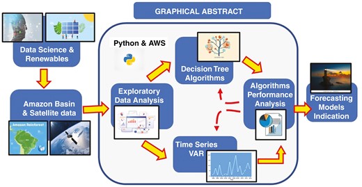
This research considers the data science (DS) workflow presented in Fig. 1. It starts by accessing the data and the associated metadata. Then, the data are checked to detect missing values, wrong typing and numbers that fall out of scale. Depending on the situation, these cases can be dropped or filled in with the mean or median of the data series to avoid introducing bias. It is a key action for exploratory data analysis (EDA) [16].
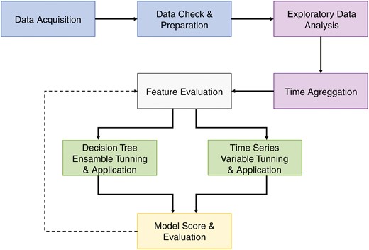
Overall data science process flow for DT and TS machine-learning models
The general behaviour among variables is depicted by graphs and visualization tools, enabling the identification of the first sets of key features. Data time aggregation is carried out by day, week and month. Before applying the TS and DT algorithms, a feature importance evaluation is performed, looking for the most significant features that explain the relationship between the target variable and the others. This action helps to save computation costs later. After data processing, each algorithm (DT or TS) is applied and scored to reduce the error or maximize the accuracy index. This process continues until the scoring strategy reaches its objective in a convergent spiral, as indicated by the dashed line in Fig. 1.
Several MLAs are set to predict the incidence of solar energy with data sources (satellites and ground stations) and local weather variables: wind speed and direction, local air humidity, season of the year, local temperature and rain accumulation. Other relevant data may be considered when evaluating the feature engineering for the DS process. Technical studies have shown correlations between solar radiation and meteorological variables and their links to the digital control of smart solar panels and energy storage devices. Therefore, feature engineering shall consider these links, along with other mathematical relations, such as the use of lag variables or other relations, studied and tested to improve prediction performance [17]. Improving the predictability of solar power generation strengthens the chances of success of investments and management during transient conditions, which may occur due to climate changes.
In the following, we detail the DT and TS algorithms used in this research.
1.1.1 DTs
DTs present cause-and-effect relationships graphically, providing a simple representation of complex phenomena in a short statement. These supervised algorithms are based on how a set of questions has been answered, which may lead to a case without a clear answer. DTs are relatively easy to understand and explain, and closely resemble human reasoning. From the root node, a set of decision nodes flows, depicting the decisions to be made. Each decision node represents a question and the leaf node, derived from the decision node, represents an answer from a binary schema (two options). Therefore, the construction of a DT requires the selection of the conditions and attributes of the tree. DTs should be continuous, allowing the outcome to be generated by analysing multiple variables. DTs can be used in a supervised approach, dealing with two separate phases: training and testing, which handle the split data from the original set [18].
A key disadvantage of DTs is the trend of ‘overfitting’, or the lack of ability to address different data from the one specifically considered because it can end up with a leaf node for each target value. Overfitting can be detected when the precision of the training phase is much higher (e.g. two or three times) than the testing one and ensemble techniques (ETs) are recommended to mitigate this issue. The core of ETs is the combination of a DT with a tool to reduce the variance or bias: bootstrap aggregation (bagging) or boosting. The first focuses on reducing the variance, while the second handles the reduction of bias.
In summary, the bagging method operates with a random sample of data in a training set, with replacement (each piece of data can be chosen more than once), allowing the training of several models (weak ones) in parallel. Ultimately, an average of all models is taken, providing a better result than a single (weak) model based on the general concept of ‘wisdom of the crowds’ or majorities. On the other hand, the boosting approach takes the sample data without replacement and the weak models are built in a series. The results of previous models are weighted for further model development, indicating the data points or features where the models need to improve. The higher the weight, the more attention is required. Some models using the ‘boosting’ concept are adaptive boosting (AdaBoost) [19], gradient boosting (GB) [20] and extreme gradient boosting (XGBoost) [21], which focuses on optimizing computer performance using distributed and parallel computing and cache memory optimization.
1.1.2 TS: vector autoregression
In a multivariate TS, variables with specific links to time may influence the measured solar incidence (target variable). It is worth noting that each variable may not be a direct consequence of its past values, but it may have some dependence on the other variables. This paper considers the vector autoregressive (VAR) model as the forecast algorithm for the TS analysis [22], following Equation (1):
where represents the target variable to be forecast at instant t, a represents the intercept and , , … represents the coefficient of lags of Y until order n.
When analysing TS data, it is crucial to check for stationarity, which refers to the constant statistical properties over time, such as mean and variance [23]. The augmented Dickey–Fuller (ADF) test is commonly used to assess stationarity [24]. The order of the VAR algorithm is another critical step in TS analysis and the Akaike information criterion (AIC) or Bayesian information criterion (BIC) tests can be used to determine the appropriate order. The order of the VAR algorithm deals with the number of variables to be considered when making the polynomial model. The order of the VAR algorithm is the shortest number of variables to achieve the lowest performance index. The Granger causality test can be performed in multivariate TS analysis to determine how explanatory variables can influence the prediction of response variables. The Johansen cointegration test verifies the existence of a significant relationship between multiple TS [25]. At the same time, the Durbin–Watson statistic is used to evaluate the autocorrelation in the residual errors of a regression analysis [26].
Table 1 summarizes the tests we used to assess stationarity, select the order of autoregressive models and verify correlations and causality among variables.
Summary of the mathematical tests associated with TS
| Test | Purpose | Null hypothesis | Statistical measure |
|---|---|---|---|
| Augmented Dickey–Fuller (ADF) | To assess stationarity in a time series | The time series has a unit root (i.e. is non-stationary) | Test statistic (e.g. t-test, F-test) |
| Akaike information criterion (AIC) and Bayesian information criterion (BIC) | To select the order of a vector autoregressive (VAR) model | Lower AIC or BIC scores indicate a better fit | N/A |
| Granger causality | To examine the causality between variables in a multivariate time series | There is no causal relationship between the variables | F-statistic |
| Johansen cointegration | To verify the existence of a significant relationship between two or more time series and examine the number of independent linear combinations of non-stationary time series that yield a stationary process | Variables are not cointegrated, meaning regression can be performed on multiple variables without falsely assuming that they are correlated | Trace statistic and the maximum eigenvalue statistic |
| Durbin–Watson | To assess the autocorrelation in the residual errors of regression analysis and determine how past values can influence predicted ones | No first-order autocorrelation in the residuals | A number between 0 and 4. A value of 2 indicates no autocorrelation. As it gets closer to 0 or 4, this indicates positive and negative autocorrelation, respectively |
1.1.3 Model performance metrics
The metric selected to evaluate the predictions was the mean absolute error (MAE), defined by Equation (2). Its dimension is the same as the variables taken, in this research, kW.h/m2 (day), from the target variable ALLSKY_SFC_SW_DWN, defined in Table 3:
Technical variables considered for the solar incidence forecast
| Variable | Unit | Description |
|---|---|---|
| ALLSKY_SFC_SW_DWN | kW.h/m² (day) | Total solar irradiance incident (direct plus diffuse) on a horizontal plane at the surface of Earth under all sky conditions |
| ALLSKY_KT | Dimensionless | A fraction representing clearness of the atmosphere and all-sky insolation transmitted through the atmosphere to strike the surface of Earth divided by the average of top of the atmosphere total solar irradiance incidents |
| PRECTOTCORR | mm/day | Precipitation-corrected—the bias-corrected average of total precipitation at the surface of Earth in water mass (including water content in snow) |
| WS10M | m/s | The average wind speed at 10 m above the surface of Earth |
| WS10M_Max | m/s | The maximum hourly wind speed at 10 m above the surface of Earth |
| WS10M_Min | m/s | Minimum hourly wind speed at 10 m above the surface of Earth |
| WD10M | Degrees | The average wind direction at 10 m above the surface of Earth |
| PS | kPa | The average surface pressure at the surface of Earth |
| RH2M | Dimensionless | The ratio of the actual partial pressure of water vapour to the partial pressure at saturation expressed as a percentage (%) |
| T2M_Min | Celsius | The minimum hourly air (dry bulb) temperature at 2 m above the ground surface in the period of interest |
| T2M_Max | Celsius | The maximum hourly air (dry bulb) temperature at 2 m above the surface of Earth in the period of interest |
| T2M | Celsius | The average air (dry bulb) temperature at 2 m above the surface of Earth |
where represents the value predicted by an algorithm, represents the real value taken from the data source and n represents the number of observations.
Another performance indicator taken was the mean value of a data group, which represents the simplest way to predict the value of that data group. The further the ratio () stays lower than 1.0, the predictor model shows to be more descriptive. The mean ratio (dimensionless) is defined by Equation (3) as follows:
1.2 Data analysis and processing
1.2.1 Data acquisition
The data core of this work deals with the Amazon basin—a vast portion of Brazil’s northern territory. More specifically, the state of Amazonas is the largest in Brazil and has faced increased deforestation from south to north due to cattle and agriculture growth. The state capital is the city of Manaus, which has an industrial pole centred on electronics, home appliances and motorcycle fabrication mostly. In this work, four medium and large cities were chosen as reference sites to take the solar incidence: Manaus, Tabatinga, Humaitá and São Gabriel da Cachoeira, covering the four extremes of the state, where the cities are near main rivers and rainforest, but with different landscape changes due to the deforestation. Table 2 presents their coordinates and population, while Fig. 2 shows the map locations [27]. For the geographical coordinates, the system used comes from the standard ISO 6709, which is suitable for mathematical processing. The cities are identified using dots.
Geographic coordinates of the four selected cities
| City | Latitude (degrees) | Longitude (degrees) | Population (hab) |
|---|---|---|---|
| Manaus | –3.101 | –60.025 | 2341.000 |
| São Gabriel da Cachoeira | +0.130 | –67.089 | 47 031 |
| Tabatinga | –4.253 | –69.935 | 42 400 |
| Humaitá | –7.500 | –63.03 | 43 500 |
| City | Latitude (degrees) | Longitude (degrees) | Population (hab) |
|---|---|---|---|
| Manaus | –3.101 | –60.025 | 2341.000 |
| São Gabriel da Cachoeira | +0.130 | –67.089 | 47 031 |
| Tabatinga | –4.253 | –69.935 | 42 400 |
| Humaitá | –7.500 | –63.03 | 43 500 |
![Location of the four cities in the Amazonas state [16]](https://oup.silverchair-cdn.com/oup/backfile/Content_public/Journal/ce/7/6/10.1093_ce_zkad065/1/m_zkad065_fig2.jpeg?Expires=1747940864&Signature=4RtMrJccLAxOPhUifLXsCKLjOF20lazNheFwI30UI02XAlVSf8weBDWHmeGj58gD9h2wYWH2jf5CxYcI9AxYujQYZMn-5tDEet3aOOyhPJ1RGi0RSG3pdyKf78ZS6rJMTw74MPAWb7BvgFJP47XZLIDsJLrOJOGEYkcTLPyo~X236YtYG8Je8uWY710TBTpySTQHJVZCQx7YRPFOiedscK6tbDYrfv8F~nlEfCVvcOQzXwwG95f4rTRzgimKt-oBuDnbaCVmdiURQcqbwBjAvKygSwUNIl6ohUAiHvZqxQu3gbTAGfW1H2TRpnc9KZDo-2~uBvyvlsA1JndbGZzRdQ__&Key-Pair-Id=APKAIE5G5CRDK6RD3PGA)
Location of the four cities in the Amazonas state [16]
Initially, the primary data source came from the Brazilian National Institute of Meteorology (INMET) website [28]. However, the data were scarce, except for Manaus. Therefore, the primary data source changed to satellite-based products from the NASA POWER Project [29], with models CERES [30] and MERRA2 [31], which take data from ground stations for support comparisons. The research period spanned from January 2013 to November 2022, corresponding to the time frame of related investigations conducted in the region [32]. The data set was acquired in the comma-separated values format and featured daily temporal resolution. It encompassed 12 variables, as listed in Table 3.
Each city data set was checked, treated and prepared for the EDA, with the number of observations: daily (3621), weekly (518) and monthly (119). As an example of the data distribution, Table 4 summarizes the data statistics for the target variable ALLSKY_SFC_SW_DWN of the four cities.
Data summary
| ALLSKY_SFC_SW_DWN | Manaus | Humaitá | SG Cachoeira | Tabatinga |
|---|---|---|---|---|
| Observed counts | 3621 | 3621 | 3621 | 3621 |
| Mean | 4.69 | 4.86 | 4.61 | 4.57 |
| Standard deviation | 1.20 | 1.04 | 1.12 | 1.08 |
| Minimum | 0.35 | 0.87 | 0.84 | 0.74 |
| 25% | 3.96 | 4.26 | 3.94 | 3.92 |
| 50% | 4.91 | 5.04 | 4.73 | 4.68 |
| 75% | 5.59 | 5.62 | 5.43 | 5.36 |
| Maximum | 7.11 | 7.23 | 7.11 | 7.17 |
In this research, we used Amazon Web Services SageMaker notebooks and Python libraries, with 4 GB and two vCPUs (ml.t3. medium), during 20 h of computing work.
In all the cases above, the missing values were filled with the median values of the same parameter to avoid data loss. This was achieved by two specific functions in the Jupyter notebooks: one to detect and count the cases, and the other to fill in the missing values. The variable with the most significant missing values for all four cities was ALLSKY_KT, with 243 cases (7%) for the daily time aggregation.
1.2.2 EDA
The EDA was carried out for the four cities to gather the order of magnitude and variance of the data. For example, Fig. 3 presents the variation of the target variable ALLSKY_SFC_SW_DWN, as a function of time, regarding the city of Manaus with a daytime aggregation.
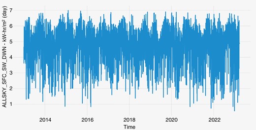
Variation of ALLSKY_SFC_SW_DWN as a function of time for Manaus
The overall outline follows a harmonic behaviour, which will be considered when exploring the TS option. Fig. 4 shows the distribution of the values of the target variable, allowing us to check that the general profile looks like a Gaussian distribution, which will be helpful when dealing with the DT options. The vertical axis computes the number of times (frequency) that the value of ALLSKY_SFC_SW_DWN [kW.h/m² (day)] is found within the data, with a daytime aggregation.
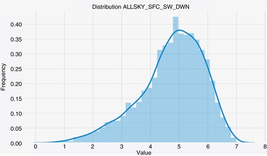
The distribution of ALLSKY_SFC_SW_DWN for Manaus with daily aggregation
The correlation matrix is presented in Fig. 5 and, with respect to the target variable, the most significant coefficients were identified with the variables ALLSKY_KT (0.887) and PRECTOTCORR (–0.645), respectively—the clearness of the atmosphere and precipitation. These numbers are important when applying the DTs and TS, and helped to define some feature engineering.
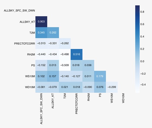
The correlation matrix of the variables related to the city of Manaus with daily aggregation
Fig. 6 shows the time variation of the target variable (left scale) and ALLSKY_KT (right scale). In general, the ALLSKY_KT variable has the same profile as the target variable, being delayed within a few time units. For the last weeks, the ALLSKY_KT has shown a constant value (horizontal line) because the median value of the series was filled in since the respective data were unavailable from the NASA source. The high correlation between ALLSKY_KT and ALLSKY_SFC_SW_DWN may be explained by the mathematical models, which consider digital images from satellites to estimate the local cloud thickness. With these data, which have some link to ALLSKY_KT, mathematical models are applied to estimate the solar irradiance in the region. This kind of graph helps to evaluate some feature engineering regarding the behaviour of the data over time, focusing on the high-order variations. The mean and standard deviation variation can be checked in three steps using normalized values.
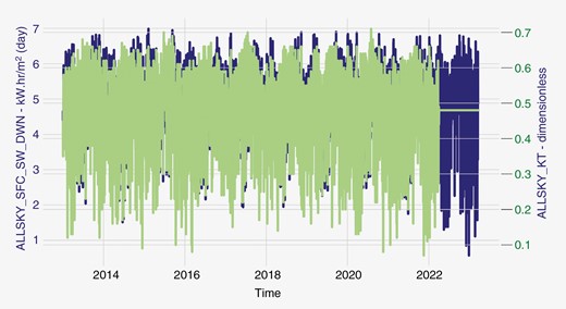
Combined presentation of ALLSKY_SFC_SW_DWN and ALLSKY_KT
1.3 Feature engineering
Regarding feature engineering, the first parameters considered were the 12 input variables, as shown in Table 1, to construct the prediction models. This first set of features was considered as the baseline. A feature importance evaluation was also done for each city with an extra tree regressor algorithm. Fig. 7 shows the feature importance for the baseline, showing the six most significant features for Manaus.
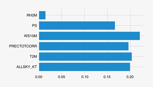
Feature importance analysis for the city of Manaus
The input variables WS10M, T2M and ALLSKY_KT have the greatest impact on the target variable (around 20%), as expected. All other variables have a lower impact. With regard to the increase in the prediction performance of the algorithms, compared with the baseline, other features were also considered, such as the local mean and standard deviation, with , and in comparison with the overall mean and standard deviation. Therefore, other additional local features were devised, such as:
local_mean_comp: the ratio between the local variable value and the local mean, or: .
mean_comp_2var: the ratio between the features above of two variables, one of them being the ALLSKY_SFC_SW_DWN.
overall_mean_comp: the ratio between the local mean, as defined above, and the overall mean until the specific value .
overall_std_comp: the ratio between the local and overall standard deviations until the specific value .
Thus, in terms of features, the major cases studied for each city and time aggregation were:
Option A: baseline (11 input variables), those listed in Table 2.
Option B: additional local features (six input variables), two with the highest feature importance and local_mean_comp, mean_comp_2var, overall_mean_comp and overall_std_comp.
Option C: additional time features (21 input variables), those listed in Table 2 plus local_mean_comp, mean_comp_2var, overall_mean_comp, overall_std_comp, day, month, day of the week, week of the year, a quarter of the year and semester.
Fig. 8 presents a flow chart on the three feature engineering options and the application of the DT and TS algorithms. Once feature engineering was selected, the DTs and TS were performed separately and the lowest MAE was identified for each city.
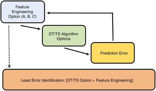
Feature engineering and DT and TS task flow
Regarding the TS model, we checked the data to confirm whether the series was stationary. If necessary, the series was modified to be stationary. After that, the training–testing split was done. The order of the model was chosen, considering the lowest value of the AIC index, and the model was fitted with the training set. Following this, the Durbin–Watson index and Granger’s causality and cointegration tests were carried out. If these test outcomes were within the test acceptance criteria, then the prediction, the MAE and the mean ratio were calculated.
Another key method is related to the number of forecasts to be done. Normally, the longer the forecast period, the higher the probability that the forecast action will exhibit larger errors in most algorithms. Therefore, this research considered different numbers of forecasting options (periods of future time): 1, 2, 3, 4, 5, 7, 10, 15 and 20. Consequently, this action impacts the training–testing split, because the number of forecasts to be done is related to the length of the test data group. For instance, in the case of 3621 observations (daytime aggregation), to have 10 predicted values, the train data group took the first 3611 values, and the test data group, the last 10. The forecast performance of the algorithm was taken from the evaluation of the test data group.
Finally, for DTs and TS, the overfitting was checked by comparison between the MAE of the training and the testing cases. If the ratio between MAE_test and MAE_train was <1.35, overfitting was not considered.
2 Results and discussion
The DTs and TS took the baseline configuration (11 input variables from the data source) for three time aggregations: daily, weekly and monthly, for every city. Table 5 presents the results of this baseline run and DT algorithms, with the lowest MAE and mean ratio, respectively. The results come from the ‘test’ data group.
DT results regarding the lowest values of MAE and means comparison
| City | Time aggregation | MAE | Mean ratio | Algorithm (best-performing) |
|---|---|---|---|---|
| Day | 0.327 | 0.585 | Adapt Boost | |
| Manaus | Week | 0.233 | 0.612 | Light Grad Boost |
| Month | 0.440 | 0.787 | Light Grad Boost | |
| Day | 0.761 | 0.703 | Light Grad Boost | |
| Humaitá | Week | 0.397 | 0.788 | Light Grad Boost |
| Month | 0.195 | 1.007 | Gradient Boost | |
| Day | 1.097 | 0.922 | Gradient Boost | |
| SG Cachoeira | Week | 0.191 | 0.769 | Adapt Boost |
| Month | 0.328 | 1.000 | Gradient Boost | |
| Day | 0.921 | 0.831 | Extreme GBoost | |
| Tabatinga | Week | 0.433 | 0.818 | Adapt Boost |
| Month | 0.418 | 0.834 | Light Grad Boost |
For the DTs and the baseline case, the lowest MAE was identified in the city of SG Cachoeira (0.191), with the weekly aggregation and the adaptive boost algorithm, with an acceptable mean ratio (0.769), without overfitting. The lowest mean ratio came from the same algorithm (0.585), in Manaus, but with a daily aggregation. The mean value of MAE was 0.470, considering all values of this indicator.
Table 6 presents a comparison, in terms of MAE, between this research and some references, showing the values with the same order of magnitude. The differences can be attributed to the diverse boundary conditions among the cases [31–34] and, by checking the data used, only Manaus has a significant difference in vegetation coverage, concentration of people and industrial activity. Thus, this situation can explain the differences in the DT and TS forecast performance. The presence of GHG and their contribution to the performance of solar energy forecast will be studied in future research.
MAE comparisons
MAE comparisons
Considering the additional local features (six input variables), Table 7 presents the city of Manaus (daily aggregation) results with the DT algorithms.
DT results with additional local features for Manaus and daily aggregation
| Algorithm | MAE | Mean ratio |
|---|---|---|
| Random forest | 0.344 | 0.425 |
| Light gradient boosting | 0.167 | 0.206 |
| Extreme gradient boosting | 0.169 | 0.209 |
| Gradient boosting | 0.275 | 0.339 |
| Adaptive boosting | 0.559 | 0.690 |
| Algorithm | MAE | Mean ratio |
|---|---|---|
| Random forest | 0.344 | 0.425 |
| Light gradient boosting | 0.167 | 0.206 |
| Extreme gradient boosting | 0.169 | 0.209 |
| Gradient boosting | 0.275 | 0.339 |
| Adaptive boosting | 0.559 | 0.690 |
Comparing these results with the baseline run, the overall results show a decrease in the MAE and mean ratio, focusing on the light gradient and extreme gradient boosting algorithms, for the same time aggregation (daily). Therefore, adopting these additional features indicates a promising potential in applying the DS tools for the current purpose.
Table 8 shows the results for Option C (21 input variables), or the third code case, with a daily aggregation, for Manaus.
DT results (Option C) for Manaus and daily aggregation
| Algorithm | MAE | Mean ratio |
|---|---|---|
| Random forest | 0.343 | 0.424 |
| Light gradient boosting | 0.221 | 0.273 |
| Extreme gradient boosting | 0.265 | 0.328 |
| Gradient boosting | 0.310 | 0.383 |
| Adaptive boosting | 0.513 | 0.634 |
| Algorithm | MAE | Mean ratio |
|---|---|---|
| Random forest | 0.343 | 0.424 |
| Light gradient boosting | 0.221 | 0.273 |
| Extreme gradient boosting | 0.265 | 0.328 |
| Gradient boosting | 0.310 | 0.383 |
| Adaptive boosting | 0.513 | 0.634 |
Compared with the baseline run, there was also a decrease in the MAE and mean ratio, again with the light gradient and extreme gradient boosting. However, comparing the second and third run options, the additional local features (six input variables) presented a small outcome. For DTs, this second run option shall be considered in the DS workflow in this research.
The best outputs of the TS option (VAR algorithm) are presented in Table 9, with their number of forecast observations and the order of the algorithm, as indicated in Equation (1) and explained in Section 1.3 above.
TS results and correlated components
| City | Time aggregation | MAE | #forecast observations | VAR order |
|---|---|---|---|---|
| Day | 0.565 | 2 | 8 | |
| Manaus | Week | 0.236 | 3 | 2 |
| Month | 0.382 | 15 | 6 | |
| Day | 0.820 | 4 | 7 | |
| Humaitá | Week | 0.384 | 4 | 2 |
| Month | 4.870* | 10* | 8* | |
| Day | 0.476 | 1 | 7 | |
| SG Cachoeira | Week | 0.188 | 4 | 2 |
| Month | 4.250* | 4* | 2* | |
| Day | 0.890 | 4 | 4 | |
| Tabatinga | Week | 0.564 | 20 | 2 |
| Month | 0.360* | 10* | 7* |
*The forecast model predicted negative values.
Most of the mean ratio values were <1.0; thus, the forecast procedure was evaluated as worth using. For TS applications, the lowest MAE was observed in SG Cachoeira (0.188) in a weekly aggregation, with several observations to be predicted of 4 and VAR model order of 2. The MAE mean value was 1.194, influenced by two cases with higher values (4.87 and 4.250). It is worth noting that the monthly aggregation in the same city produced negative predicted values (indicated by the * in Table 9), which does not make sense; therefore, this specific case shall not be considered. Taking these two major cases from the list, the mean value of MAE is 0.533. Comparing this scenario to the related work presented in Table 6, as carried out for DTs, the TS approach produces results of the same order of magnitude. To improve the performance of the prediction algorithms, concentrating on the Manaus case, the use of additional features contributed positively. The lowest MAE was 0.167, with a mean ratio of 0.206—a reduction of 28%. It is key to highlight the reduction of features, from baseline to this additional local one, which contributed to reducing the complexity of the model, preserving the initial variables with the highest feature importance. The mean MAE value was 0,300 and the mean ratio was 0.373, without overfitting. On the other hand, when the number of variables was increased, the lowest MAE was 0.221 with a mean ratio of 0.273. Compared with the previous case, MAE increased by 30%. The mean MAE value was 0.330. Compared with the first two cases, it showed a worse MAE performance, although the mean ratio was reasonable or <0.5. Therefore, an increase in the number of features should be avoided.
3 Conclusions
When the two mathematical approaches were compared, both showed MAE of the same magnitude, though the DT approach was ~30% smaller. The best MAE (0.167) came from applying the light gradient boosting with feature engineering of Option B. For this specific result, the mean ratio was 0.206, indicating that the DT procedure rounds one-fifth of the forecast method based on the mean of the overall target variable (the easiest predictor). This allows us to conclude that the DT was shown to be a reasonable tool for prediction. Equally importantly, it is worth noting that the light gradient boosting had no overfitting.
Specifically for the TS approach, the lowest MAE was 0.188 for weekly aggregation and four forecast observations, with a VAR model of order 2. The low-order models (<3) performed two or three times better than the high-order ones (≥4). Although small MAEs were also obtained, they were associated with ‘negative’ predicted values in some TS configurations, as seen in Humaitá, Tabatinga and SG Cachoeira, which requires extra attention when applying TS.
The DS task flow above showed coherence with the references. It may be replicated in similarly remote locations or regions in India, Indonesia and Africa [37] to forecast solar incidence based on satellites as an alternative to the absence of land stations or faulty measurement devices.
In a vision of future work, the presence of GHG should be considered, as the number of rainforest fires has increased, mainly due to deforestation. Equally importantly, the present methodology will be used to evaluate the substitution of thermal electricity generation for oil fuels in the region. The input can be increased with data from environmental monitoring towers, focusing on CO2 and methane, for instance, along other ground data sources. Again, the limitations on the data availability and quality, due to station coordinates and measuring/transmission troubles, can be addressed in more detail.
Acknowledgements
The authors want to thank São Paulo Research Foundation and the Ministry of Defense—Amazon Protection System (SIPAM).
Author contributions
Conceptualization, A.M., M.T., F.A. and P.C.; methodology, A.M. and P.C.; software and validation, A.M., M.T. and P.C.; investigation, A.M.; writing---original draft preparation, A.M, M.T. and F.A.; writing---review and editing, A.M., M.T., F.A. and P.C.; supervision, P.C.; project administration, P.C. All authors have read and agreed to the published version of the manuscript.
Conflict of interest statement
The authors declare no conflict of interest.
Funding
The authors acknowledge the support of the Research Centre for Greenhouse Gas Innovation (RCGI), hosted by University of São Paulo (USP) and sponsored by FAPESP (grants #2014/50279-4 and #2020/15230-5, #2022/07974-0) and Shell Brasil, and the strategic importance of the support given by Brazil’s National Oil, Natural Gas and Biofuels Agency (ANP) through the R&D levy regulation. Equally importantly, Felipe Almeida is sponsored by the National Council for Scientific and Technological Development (CNPq), grant #140253/2021-1.
Data Availability
The data underlying this article are available in Zenodo.org, at https://doi.org/10.5281/zenodo.7539131 [38] and https://doi.org/10.5281/zenodo.7539155 [39].
