


Summary
With the availability of limited resources, innovation for improved statistical method for the design and analysis of randomized controlled trials (RCTs) is of paramount importance for newer and better treatment discovery for any therapeutic area. Although clinical efficacy is almost always the primary evaluating criteria to measure any beneficial effect of a treatment, there are several important other factors (e.g., side effects, cost burden, less debilitating, less intensive, etc.), which can permit some less efficacious treatment options favorable to a subgroup of patients. This leads to non-inferiority (NI) testing. The objective of NI trial is to show that an experimental treatment is not worse than an active reference treatment by more than a pre-specified margin. Traditional NI trials do not include a placebo arm for ethical reason; however, this necessitates stringent and often unverifiable assumptions. On the other hand, three-arm NI trials consisting of placebo, reference, and experimental treatment, can simultaneously test the superiority of the reference over placebo and NI of experimental treatment over the reference. In this article, we proposed both novel Frequentist and Bayesian procedures for testing NI in the three-arm trial with Poisson distributed count outcome. RCTs with count data as the primary outcome are quite common in various disease areas such as lesion count in cancer trials, relapses in multiple sclerosis, dermatology, neurology, cardiovascular research, adverse event count, etc. We first propose an improved Frequentist approach, which is then followed by it’s Bayesian version. Bayesian methods have natural advantage in any active-control trials, including NI trial when substantial historical information is available for placebo and established reference treatment. In addition, we discuss sample size calculation and draw an interesting connection between the two paradigms.
1. Introduction
The randomized controlled trials (RCTs) are traditionally the gold standard for judging the benefits of treatment for a disease under idealistic condition. According to the requirements set by the regulatory agencies (e.g., FDA, 2016; EMA, 2005), drug developers need to demonstrate evidence of efficacy and safety of an intervention through well-designed randomized placebo-controlled trial/s (RCTs). However, in the presence of an established treatment regime conducting placebo-controlled trial is unethical. Instead, experimental treatment is compared with an active control or reference treatment/drug/intervention. Most of such active comparator trials are superiority trials. However, when superiority of the experimental intervention is not clear, yet it poses certain attractive properties, one may resort to a non-inferiority (NI) trial. The objective of efficacy seeking NI trial is to establish that an experimental treatment is non-inferior to an active comparator within a small, pre-specified margin (or NI margin), and at the same time retains a substantial portion of the active controls effect in the current trial (D’Agostino Sr and others, 2003). The choice of this NI margin has been an area of major concern and some broad outlines have been provided by regulatory agencies (ICH Steering Committee, 1998, 2000; FDA, 2016; EMA, 2005). The following references (FDA, 2016; Hung and Wang, 2004; Schumi and Wittes, 2011) provide a detailed discussion on NI margin that must be constructed based on the past performance of active control. Sometime an intervention after passing superiority test for efficacy, additionally also tested for NI for safety, however that is not the main focus of this article (Tsong and Zhang, 2007; Lu and others, 2018).
For the ethical reason discussed above, NI trials mostly lack a placebo arm. Hence, such two-arm NI trials make some important assumptions regarding assay sensitivity and constancy. The validity of the resulting inference depends heavily on external validation. Assay sensitivity (AS) of a clinical trial is defined in its ability to distinguish an effective treatment from a less effective/ineffective one as defined by the ICH guideline (ICH Steering Committee, 1998, 2000). Moreover, it is also required that the effect size of the active control over placebo in the historical placebo-controlled trial holds in the current NI trial (i.e., constancy), otherwise efficacy of the experimental treatment over putative placebo cannot be shown. Kieser and Stucke (2016) mentioned several other factors that often plague two-arm NI trials. To alleviate some of these issues and if ethically acceptable and practically feasible, it is recommended by EMA (2005) to include a placebo arm in the current trial, resulting in a three-arm trial often known as “gold-standard” design. In Frequentist setup, Pigeot and others (2003) first proposed an approach where NI margin is adaptively formulated as the pre-specified negative fraction of the unknown effect size of the reference treatment over placebo in the current three-arm trial. Such formulation of the NI margin, called the fraction margin approach, is also known as “effect retention.” This approach was extended by Kieser and Friede (2007) and Chowdhury and others (2018b) for the binary outcome, Mielke and others (2008) for censored exponentially distributed outcome, Ghosh and others (2017) for non-normal continuous outcome, Stucke and Kieser (2013) and Mütze and others (2016) for the count outcome to name a few.
1.1. Background and motivating example
A three-arm trial via fraction margin approach is a two-step process. In the first step, one must show that superiority of the reference over placebo, i.e., the AS condition holds. If this is successful, one proceeds to test NI of the experimental treatment. Due to the hierarchical structure of the multiple testing problem (AS and NI) though one do not need to adjust for type-I error, however, the pretest for assay sensitivity may lead to a reduction in power when testing for NI. This fact was demonstrated clearly in Kieser and Friede (2007). A possible alternative is proposed by Hida and Tango (2013), where they suggested joint testing of AS and NI. This approach requires joint rejection of AS and NI null hypotheses to claim NI (with AS) leading to Intersection–Union testing (IUT). Though logical and can be tightly controlled (for type-I error) the IUT under Frequentist setup may lead to biased test (Berger, 1997). This is discussed in detail by Chuang-Stein and others (2007) in the superiority trial context. In this article based on Frequentist approach we have developed first, a more powerful test based on conditional principle for fraction margin based NI testing.
Since NI trials involve active control that has been well established in the past, the availability of historical information is almost guaranteed. Bayesian paradigm provides a natural path to combine information from various historical trials as prior and then to combine them with the current trial. This has the possibility of reducing sample size and cost burden. Bayesian approaches have been predominantly used in clinical trials, particularly in the NI trials since long past (e.g., see Simon, 1999; Ghosh and others, 2011, 2016; Gamalo and others, 2016, 2014). Bayesian approach for NI trial for two-arm can be found in Gamalo and others (2011), Chowdhury and others (2018a) and for three-arm can be found in Ghosh and others (2011), Ghosh and others (2016). To the best of our knowledge no literature exists for NI testing for count outcomes under Bayesian paradigm. Even from the Frequentist approach the papers are only handful. Albeit as mentioned in Stucke and Kieser (2013), the existence of count type outcome is not very uncommon. Examples include relapse-remitting count in multiple sclerosis (MS) trial (Friede and Schmidli, 2010; Noseworthy, 2003; Sormani and others, 2001); lesion count in cancer trial (McIntosh, 2001; Xie and Aickin, 1997); number of attacks in migraine trial (Silcocks and others, 2010); number of manic episodes in bipolar trial (Soeiro-de Souza and others, 2013); post-discharge adverse events (Tsilimingras and others, 2015) to name a few. Along with a novel and more powerful conditional Frequentist approach in this article, we also propose both exact and an approximate Bayesian approach for testing the NI hypothesis for count outcomes in three-arm trial. Effective sample size is calculated using all procedures to make a comparative analysis.
Our motivation for developing both Frequentist and Bayesian tests comes from a clinical trial dataset (Calabrese and others, 2012) on MS where primary outcome is counts of cortical inflammatory lesions (CLs). Recent studies have shown that CLs may have a major role in determining disability in patients with MS. Some of the critical symptoms of CLs include epilepsy, memory loss in relapsing-remitting multiple sclerosis (RRMS) patients, cortical atrophy in primary progressive MS, etc. The original dataset comprises of patients who were untreated or treated with different disease modifying drugs (DMDs). The objective of the study was to assess the effects of the DMDs compared with no therapy (placebo). The patients with RRMS were enrolled in a 2-year prospective, randomized, single-centric study. There were |$50$| patients who did not receive any therapy for the 2 years of the follow-up period, while the remaining patients who were part of the clinical study, received the respective DMDs. These patients were evaluated at baseline, at 12 and 24 months after the treatment. Table 1 shows the frequencies of the new CLs developed by these patients with MS after 1 year and 2 years of their treatment with the DMDs. As evident the primary response is count type, with good fit to Poisson distribution via Index of Dispersion test (Gbur, 1981) for all arms. We have applied our proposed test procedures to determine NI of the DMD glatiramer acetate (GA) (|$E$|) over subcutaneous interferon (IFN) beta-1a (|$R$|) for both 1- and 2-year data. The detailed illustrations are in Section 6.
Frequencies of new MRI CLs over 1 and 2 years. |$N$| denotes sample size.
| 1 year | 2 years | ||||||
|---|---|---|---|---|---|---|---|
| Arm | Counts | Frequencies | |$N$|, Mean, Var | Arm | Counts | Frequencies | |$N$|, Mean, Var |
| |$P$| | 0 | 13 | 50, 1.6, 1.2 | |$P$| | 0 | 9 | 50, 3.0, 2.6 |
| |$\geq1$| | 37 | |$\geq1$| | 41 | ||||
| |$R$| | 0 | 34 | 46, 0.4, 0.49 | |$R$| | 0 | 22 | 46, 0.8, 0.6 |
| |$\geq1$| | 12 | |$\geq1$| | 24 | ||||
| |$E$| | 0 | 24 | 48, 0.8, 1.0 | |$E$| | 0 | 18 | 48, 1.3 , 1.21 |
| |$\geq1$| | 24 | |$\geq1$| | 30 | ||||
The rest of the article is organized as follows. In Section 2, we give the NI hypothesis and existing Frequentist methods for testing the count data. We also introduce our proposed more powerful conditional testing in this section. In Section 3, we propose a novel Bayesian methodology for the same. We consider both conjugate and non-conjugate priors incorporating the condition of AS. In Section 4, the power and sample size calculations are discussed in detail for Frequentist approach, Bayesian normal approximation, and exact Bayesian methods. Section 5 presents the simulation results along with the power curves. Finally in Section 6, we apply our proposed Bayesian methodology for NI testing on this clinical trial dataset. The article concludes with discussion and future direction in Section 7. All proofs and additional simulation results are provided in Supplementary Appendix available at Biostatistics online.
2. Frequentist approach for NI testing
2.1. Existing Frequentist approaches
Mütze and others (2016) developed NI hypothesis testing where count outcome assumed to follow a negative binomial distribution. They constructed the test statistic for testing NI hypothesis by considering the maximum likelihood (ML) estimate of the linear contrast in |$H_{0}$| (in 2.3) given by, |$ T=\hat{\lambda}_{E}-\theta\hat{\lambda}_{R}-\left(1-\theta\right)\hat{\lambda}_{P}, $| where |$\hat{\lambda}_{l}={X_{l}}/{n_{l}t_{l}}$| is the maximum likelihood estimate (MLE) of |$\lambda_{l}$|, |$l\in\left\{ E,R,P\right\} $|. The variance of the test statistic is given as |${\rm Var}\left(T\right)={\lambda_{E}}/{n_{E}t_{E}}+\theta^{2}{\lambda_{R}}/{n_{R}t_{R}}+\left(1-\theta\right)^{2}{\lambda_{P}}/{n_{P}t_{P}}. $| Both ML and restricted maximum likelihood (RML) estimation techniques can be adopted to estimate |${\rm Var}(T)$|. The RML estimator can be obtained subject to the constraint |$\lambda_{E}-\theta\lambda_{R}-\left(1-\theta\right)\lambda_{P}=0$|. Mütze and others (2016) also derived asymptotic sample size formulae along with optimal sample size allocation considering both balanced and unbalanced designs albeit in the Frequentist set up. For a two-arm trial, Stucke and Kieser (2013) derived the statistical test procedure using RML estimator and obtained approximate sample size formulae under the Frequentist set up. Note, this approach of NI testing is valid provided the AS null hypothesis has already been rejected first. Hence, the step for NI testing is always a conditional test. However, this AS conditioning is not used in any of the existing approach of Frequentist test. We have shown mathematically that if the pretested AS condition is used properly in the second step (i.e., in NI testing), this could lead to a more powerful test with considerable savings in sample size.
2.2. Proposed Frequentist approach
This strategy is proved to be quite useful in many practical applications (Huang and others, 2011; Kulldorff, 1997). Since working with product of random variables in (2.4) is little cumbersome, one can further show that |$f(T_{{\rm RML}})\simeq {f(T_{{\rm ML}}|\hat{\lambda}_{R, {\rm ML}}\,{>}\,\hat{\lambda}_{P,{\rm ML}})} \times Pr[\hat{\lambda}_{R,{\rm ML}}\,{>}\,\hat{\lambda}_{P,{\rm ML}}]$|. It is easy to prove that |$Pr[\hat{\lambda}_{R,{\rm ML}}\,{>}\,\hat{\lambda}_{P,{\rm ML}}]$| is a constant value which can be absorbed as a proportionality constant. Hence, for all practical purposes, one can consider the distribution of the test statistic, |$f(T_{{\rm ML}}|\hat{\lambda}_{R}\,{>}\,\hat{\lambda}_{P}) \propto f(\hat{\lambda}_{E,{\rm ML}}-\theta \hat{\lambda}_{R,{\rm ML}}-(1-\theta) \hat{\lambda}_{P,{\rm ML}}|\hat{\lambda}_{R,{\rm ML}}\,{>}\,\hat{\lambda}_{P,{\rm ML}})$|. For notational simplicity from now onwards, we denote the ML estimate |$\hat{\lambda}_{l,{\rm ML}}$| by |$\hat{\lambda}_{l}$|, |$l \in \{E,R,P\}$|. This leads to the modified test statistic for NI testing: |$W=(\hat{\lambda}_{E}-\theta\hat{\lambda}_{R}-(1-\theta)\hat{\lambda}_{P}|\hat{\lambda}_{R}\,{>}\,\hat{\lambda}_{P}) = \left(U-\theta V|V\,{>}\,0\right)$|. Under the asymptotic normality of |$W$|, we have |$ {(W-\mu_{w})}/{\sigma_{w}}\sim AN\left(0,1\right)$|, where |$\mu_{w}\mbox{ and }\sigma_{w}^{2}$| are the mean and variance of |$W$|, respectively.
Under conditional normal approximation, the mean |$\mu_{w}$| and variance |$\sigma_{w}^{2}$| of |$W=\hat{\lambda}_{E}-\theta\hat{\lambda}_{R}-(1-\theta)\hat{\lambda}_{P}|\hat{\lambda}_{R}\,{>}\,\hat{\lambda}_{P}$| are given by |$ \mu_{w}= \mu_{U}+\sigma_{U}\frac{\rho}{c}\phi\left(d\right)-\theta \left(\mu_{V}+\sigma_{V}\frac{1}{c}\phi\left(d\right)\right), \sigma_{w}^{2}= \sigma_{U}^{2}\left[1+\frac{\rho^{2}}{c}d\phi\left(d\right)-\left(\frac{\rho}{c}\phi\left(d\right)\right)^{2}\right] + \theta^2 \sigma_{V}^{2}\left[1-\frac{\phi\left(d\right)}{c}\left(\frac{\phi\left(d\right)}{c}-d\right)\right] - 2\theta\left[\sigma_{U}\sigma_{V}\frac{\rho}{c}\left(c+d\phi\left(d\right)\right)+ \sigma_{U}\mu_{V}\frac{\rho}{c}\phi\left(d\right) \right.$||$\left. + \sigma_{V}\mu_{U}\frac{1}{c}\phi\left(d\right)+\mu_{U}\mu_{V} -\left(\mu_{U} +\sigma_{U}\frac{\rho}{c}\phi\left(d\right)\right) \left(\mu_{V}+\sigma_{V}\frac{1}{c}\phi\left(d\right)\right)\right], \mbox{ where } \mu_{U} =\lambda_{E} -\lambda_{P},\mbox{ }\mu_{V}=\lambda_{R}-\lambda_{P},\mbox{ }\sigma^2_{l}=\frac{\lambda_{l}}{n_{l}} \mbox{ for }l \in \{E,R,P\},\mbox{ } d =-\frac{\mu_{V}}{\sigma_{V}}, c =1 -\Phi\left(d\right), \mbox{ }\sigma_{U}^{2} =\sigma_{E}^{2}+\sigma_{P}^{2},\mbox{ }\sigma_{V}^{2} =\sigma_{R}^{2}+\sigma_{P}^{2},\mbox{ and }\rho =\frac{Var(\hat{\lambda}_{P})}{\sqrt{Var\left(U\right)Var\left(V\right)}}=\frac{\sigma_{P}^{2}}{\sqrt{\sigma_{U}^{2}\sigma_{V}^{2}}}. $|
Proof: See Supplementary Appendix A available at Biostatistics online.
Now under |$H_{0}$|, let us denote |$\lambda_{E}\mbox{ by }\lambda_{E}^{\rm null}$| and under |$H_{1}$| denote |$\lambda_{E}\mbox{ by }\lambda_{E}^{\rm alt}$| as point alternative. Since |$\lambda_{E}^{\rm null}$| satisfies |$\lambda_{E}^{\rm null}-\theta \lambda_{R}-(1-\theta) \lambda_{P}=0$|, the expression of |$\lambda_{E}^{\rm null}$| can be obtained via |$ \lambda_{E}^{\rm null} =\lambda_{P}+\theta\left(\lambda_{R}-\lambda_{P}\right). $| Under |$H_{1}$|, |$\lambda_{E}^{\rm alt}$| satisfies |$\lambda_{E}^{\rm alt}-\theta\lambda_{R}-(1-\theta)\lambda_{P}\,{>}\,0\Rightarrow(\lambda_{E}^{\rm alt}-\lambda_{P})\,{>}\,\theta(\lambda_{R}-\lambda_{P})$|. Since |$\lambda_{E}$| is involved in the expression of the mean and variance of |$W$|, we denote |$E\left(W\right)$| and |${\rm Var}\left(W\right)$| under |$H_{0}$| by |$\mu_{w}^{\rm null}$| and |$\sigma_{w}^{2\rm null}$| and under |$H_{1}$|, by |$\mu_{w}^{\rm alt}$| and |$\sigma_{w}^{2 \rm alt}$|, respectively. Thus, we have |$ {(W-\mu_{w}^{\rm null})}/{\sigma_{w}^{\rm null}} \sim AN\left(0,1\right)\mbox{ under }H_{0}\mbox{ and } {(W-\mu_{w}^{\rm alt})}/{\sigma_{w}^{\rm alt}} \sim AN\left(0,1\right)\mbox{ under }H_{1}. $| In Frequentist approach, the critical region of the test is given by |$W\,{>}\,k^{*}_{\alpha}$|, where |$k^{*}_{\alpha}$| is obtained by assuming a test of size |$\alpha$|: |$ P_{H_{0}}\left(W\,{>}\,k^{*}_{\alpha}\right) =\alpha\Rightarrow k^{*}_{\alpha}=\mu_{w}^{\rm null}+z_{1-\alpha}\sigma_{w}^{\rm null}, $| where |$z_{1-\alpha}$| is the |$100\left(1-\alpha\right)\%$| percentile point of the |$N\left(0,1\right)$| distribution. Traditionally, the value of |$\alpha$| is chosen to be |$0.025$| (other choices are possible too). The expression of the power of the test is given by |$ P_{H_{1}}\left(W\,{>}\,k^{*}_{\alpha}\right)=1-\Phi({(k^{*}_{\alpha}-\mu_{w}^{\rm alt})}/{\sigma_{w}^{\rm alt}}). $|
At a fixed |$\alpha $| and sample size |$N(=n_E+n_R+n_P)$|, proposed conditional test statistic |$ (W) $| has more power than the existing marginal test statistic |$ (T) $| for testing NI hypothesis in (2.3).
Proof: See Supplementary Appendix B available at Biostatistics online.
This lemma shows that there is effective power gain in the conditional test or conversely speaking, to attain a fixed power, the conditional test requires smaller sample size. Though for simplicity, the proof is given for equal allocation case, it can be easily extended for more general unequal allocation case. As observed in the Section 4.5, this power difference is substantial when the gap between |$ \lambda_R $| and |$ \lambda_P $| is small. In Supplementary section available at Biostatistics online, we have provided additional simulation result to demonstrate this fact. It should be also noted that this lemma is generalizable for continuous as well as for binary outcome with slightly different algebra, indicating the fact that our proposed conditional test should be de facto standard for Pigeot’s fraction margin approach irrespective of the outcome types.
3. Bayesian approaches for NI testing
As indicated in Section 1, availability of considerable prior information is almost guaranteed in any active control trial and NI RCT is not an exception. Albeit, the usage of these historical information via the Frequentist approaches is rather limited. Bayesian approach provides a natural path to leverage this historical data which may result in substantial effective sample size gain. However, to the best of our knowledge no Bayesian methodology paper exists for any three-arm trial with count type endpoints. In this section, we discuss an exact Bayesian and an approximation-based Bayesian method for NI testing involving Poisson rates. Note, we did not develop here Bayesian approach for existing Frequentist approach of Mütze and others (2016). However, as we proposed a more powerful Frequentist test in Section 2.2, our Bayesian development closely follows that procedure.
As stated earlier, the NI margin is constructed as the negative fraction of the unknown difference of the count rate of responses in the reference and the placebo arm. We consider |$\theta\geq0.5$| to test for the NI of |$E$| relative to |$R$| with two different prior scenarios, including the conjugate prior where the AS condition |$\left(\lambda_{R}\,{>}\,\lambda_{P}\right)$| is directly incorporated. This restriction reflects that the NI study is being carried out under the similar condition as that of the former studies in which the efficacy of the active control was proved, and it still retains its effect over placebo. This is a very realistic assumption because if the current trial is similar to the historical trial then the effect of reference drug over placebo should be constant in both the current and the historical trial (constancy assumption). In the following section, we discuss both the conjugate and non-conjugate prior settings. In case there is no available prior information, flat non-informative prior is assigned to |$\lambda_{l}$| which includes Jeffreys prior and other priors with adjusted parameters yielding large variance.
3.1. Exact Bayesian approach
3.1.1. Conjugate Gamma prior
The Markov chain Monte Carlo (MCMC) samples can be easily generated from this joint posterior distribution. The hyper-parameters |$\alpha_{l}$| and |$\beta_{l}$|, |$l\in\{E,R,P\}$| can be chosen depending on how much prior information is available. In the absence of prior information from historical placebo-controlled trial, they are chosen to be vague. The mean |$\left(\mu\right)$|, mode |$\left(\mu^{0}\right)$|, and variance |$\left(\sigma^{2}\right)$| of |$\text{Gamma}\left(\alpha,\beta\right)$| are given as |$ \mu ={\alpha}/{\beta}$|, |$\mu^{0}={(\alpha-1)}/{\beta}$|, and |$\sigma^{2}={\alpha}/{\beta^{2}}$|. For the informative priors, the variance is made smaller making priors to be more specific.
3.1.2. Non-conjugate prior
The posterior is not in the closed form and a Metropolis–Hastings acceptance–rejection sampling is required with a proposal density to generate posterior samples (Gelman and others, 2014). A convenient proposal density could be |$ \text{Gamma} $| distribution with appropriately chosen priors. In our simulation, we use “rjags” (R-package; Plummer and others, 2016) to generate the samplers from the posterior density.
Following Pigeot and others (2003) and Ghosh and others (2011), we continue to assume that AS condition |$(\lambda_R\,{>}\,\lambda_P)$| is tested in Step 1, before proceeding to test for NI. As a result truncated priors are chosen in Step 2, i.e., at NI testing. This assumption explicitly reflects the fact that active control still retains some of its effect over placebo. In a situation where this assumption is questionable, it is not advisable to carry out a three-arm NI trial, rather a superiority trial of the new treatment over placebo is more realistic.
3.1.3. Test procedure
3.2. Approximate Bayesian approach
Note that in the exact Bayesian approach, the posterior sample generation is necessary to carry out the Bayesian inference which is often computationally intensive. Here, we propose an approximation-based Bayesian approach for NI testing incorporating the AS condition that gives closed form of the posterior probability and hence, saves the computation time of the MCMC sample generation from posterior distribution. Consider the |$ \text{Gamma} $| prior for the rate |$\lambda_l$| in each arm, that is, |$\lambda_l\sim \text{Gamma}\left(\alpha_l,\beta_l\right)$| and assume that the responses are distributed as Poisson; that is, |$X_l\sim \text{Poisson}\left(n_l\lambda_l t_l\right)$| for |$l\in\{E,R,P\}$|. The Frequentist test statistic for testing the hypothesis in equation (2.3) is given by |$ T={X_{E}}/{n_{E}t_{E}}-\theta{X_{R}}/{n_{R}t_{R}}-(1-\theta){X_{P}}/{n_{P}t_{P}}. $| For the sake of simplicity, we take |$t_{l}=1$|, |$l\in \{E,R,P\}$|. Under asymptotic normality assumption, we have |$T|\mu_{T}\sim AN\left(\mu_{T},\sigma_{T}^{2}\right)$|, where |$ \mu_{T}=\lambda_{E}-\theta\lambda_{R}-(1-\theta)\lambda_{P}=(\lambda_{E}-\lambda_{P})-\theta(\lambda_{R}-\lambda_{P}) $| and |$ \sigma_{T}^{2}={\lambda_{E}}/{n_{E}}+\theta^{2}{\lambda_{R}}/{n_{R}}+\left(1-\theta\right)^{2}{\lambda_{P}}/{n_{P}}. $| Putting Normal prior on |$\mu_{T}$|, we have |$\mu_{T}\sim AN\left(\mu^{*},\sigma^{*2}\right)$|, where |$\mu^{*}=E\left(\mu_{T}\right)=\mu_{E}-\theta\mu_{R}-\left(1-\theta\right)\mu_{P}$| and |$\sigma^{*2}=\sigma_{E}^{2}+\theta^{2}\sigma_{R}^{2}+(1-\theta)^{2}\sigma_{P}^{2},$||$\mu_{l}$| and |$\sigma_{l}^{2}$|, |$l\in\{E,R,P\}$| are the respective mean and variance of the |$ \text{Gamma} $| prior for the Poisson rates. Next, we bring in the condition of AS |$(\lambda_{R}\,{>}\,\lambda_{P})$|. So instead of taking prior on |$\mu_{T},$| we take prior on |$\nu_{T}\equiv\left(\mu_{T}|\lambda_{R}\,{>}\,\lambda_{P}\right)$|. Assume that |$\nu_T\sim AN\left(\mu_{\nu}^{*},\sigma_{\nu}^{*2}\right)$| and the posterior, |$\nu_T|\text{Data} \sim AN\left(\widetilde{\mu}_{T}\widetilde{\sigma}_{T}^{2},\widetilde{\sigma}_{T}^{2}\right)$|. We refer to Arnold and Beaver (1993) for the detailed derivation of |$\mu_{\nu}^{*},$||$\sigma_{\nu}^{*2}$|, |$\widetilde{\mu}_{T}$|, and |$\widetilde{\sigma}_{T}^{2}$| (see also Supplementary Appendix C available at Biostatistics online). The Bayesian decision rule for the experimental treatment to be non-inferior to the active comparator is given by Gamalo and others (2014)|$: P\left(\nu_{T}\geq0|\text{Data}\right)\,{>}\, p^{*}, $| where |$p^{*}$| is the pre-specified clinically reasonable constant.
4. Power and sample size determination
We address the problem of calculating the sample size for the assessment of NI to attain a desired power using three approaches described in Sections 2 and 3. The normal approximation-based approaches do not require any simulation for the estimation of the power function as it can be expressed in a closed form (as presented in the following subsections). However, the exact Bayesian approach requires the simulation technique to obtain the empirical power which is then set to a desired level to calculate the corresponding sample size. In our sample size calculation, we consider |$t_{l}=1,$||$l\in\{E,R,P\}$|. We want to determine the sample size |$n_{l},$||$l\in\{E,R,P\}$| setting the power at |$\left(1-\beta\right)$|, |$\beta$| is the pre-specified type-II error. We assume |$n_{E}=n$|, |$n_{R}=r_{1}n$|, and |$n_{P}=r_{2}n$|, where |$r_{1}$| and |$r_{2}$| determine the allocation of the sample sizes in the reference and the placebo arms, respectively, relative to the experimental arm. The total sample size in that case would be |$N=n\left(1+r_{1}+r_{2}\right)$|. In the following sub-section, we discuss the power and sample size calculation under the proposed Frequentist, approximation-based Bayesian, and exact Bayesian approaches.
4.1. Frequentist approach
Setting |$\beta$| at |$20\%$|, that is, to have at least |$80\%$| power and at fixed |$\alpha(=0.025)$|, |$n$| is determined from (4.1). We vary |$\lambda_{E}^{\rm alt}$| to get the minimum sample size satisfying at least |$80\%$| power for each |$\lambda_{E}^{\rm alt}$|.
4.2. Exact Bayesian approach
The sample size can be obtained by setting the estimated power to be at least |$100(1-\beta)\%,$||$\beta$| is usually chosen to be |$0.2$|. We note here that since under the exact Bayesian approach the estimation of power involves generating samples from posterior distributions, there could be minor fluctuation in the estimated sample size.
4.3. Approximate Bayesian approach
A similar derivation albeit for two-arm NI trial for binary outcome can be found in Gamalo and others (2014). Now, “|$n$|” can be solved from (4.5) by setting |$\beta=20\%$| and simultaneously satisfying condition (C1) for each |$\lambda_{E}^{\rm alt}$| (which is included in |$\mu_{T}^{\rm alt}$|).
4.4. Sample size under different allocation
We determine the approximate sample size to attain a power of |$1-\beta=0.8$| under three different allocation scenarios for |$\left(E,\mbox{}R,\mbox{}P\right)$|: |$\left(1{:}1{:}1\right)$|, |$\left(2{:}2{:}1\right)$|, and |$\left(3:2:1\right)$| of the total sample size |$N(=n(1+r_{1}+r_{2}))$|. We express the sample sizes in the reference and the placebo group as proportions |$r_{1}$| and |$r_{2}$| of the sample size |$n_{E}$| in the experimental group. Hence, for the allocation |$\left(1:1:1\right),$||$r_{1}=r_{2}=1$|; for |$\left(2{:}2{:}1\right)$|, |$r_{1}=1\mbox{ and }r_{2}=\frac{1}{2}$|; and for |$\left(3{:}2:1\right)$| the values are |$r_{1}=\frac{2}{3}$| and |$r_{2}=\frac{1}{3}$|. Type-I error or |$\alpha=0.025$| is kept fixed for the Frequentist approach, while for Bayesian approach we also made sure the equations (4.4) and (4.5) hold simultaneously for fixed |$(\alpha, \beta )$|. In practice, |$\theta$| is chosen in |$[0.5,1)$|, to ensure retention of at least |$50\%$| effect of the active control. The sample sizes are presented for |$\theta=0.8$| and |$0.75$| and for a range of |$\lambda_{E}$| keeping |$\lambda_{R}=21$| and |$\lambda_{P}=7$| in Table 2. Other values of |$\lambda$|’s are also possible satisfying the restriction |$\lambda_{R}\,{>}\,\lambda_{P}$|.
Sample sizes based on exact and approximate approaches to achieve a power of |$80\%$| for |$\theta=0.8$| and |$0.75$|, |$\alpha=0.025$| and keeping |$\lambda_R=21$| and |$\lambda_P=7$| under three different allocations. The simulated power (|$ \hat{\phi} $|) and estimated average type-I error (|$ \hat{\alpha} $|) for exact Bayesian approach under non-informative Gamma prior are also reported to show that calculated sample size is adequate to guarantee |$80\%$| power except for minor numerical fluctuation. Note, Frequentist type-I error is always strictly maintained at |$\alpha= 0.025$| by equation 4.1.
| Frequentist normal | Approximate Bayesian | Exact Bayesian | ||||||||||||
|---|---|---|---|---|---|---|---|---|---|---|---|---|---|---|
| |$E$| | |$R$| | |$P$| | |$\theta$| | |$\lambda_{E}$| | |$n_{P}$| | |$N$| | |$ \hat{\phi} $| | |$n_{P}$| | |$N$| | |$ \hat{\phi} $| | |$n_{P}$| | |$N$| | |$ \hat{\phi} $| | |$ \hat{\alpha} $| |
| 20.0 | 79 | 237 | 0.802 | 78 | 234 | 0.801 | 79 | 237 | 0.802 | 0.0215 | ||||
| 19.7 | 113 | 339 | 0.802 | 112 | 336 | 0.798 | 112 | 336 | 0.808 | 0.0222 | ||||
| 0.80 | 19.4 | 176 | 528 | 0.790 | 175 | 525 | 0.795 | 175 | 525 | 0.796 | 0.0225 | |||
| 19.1 | 312 | 936 | 0.795 | 310 | 930 | 0.797 | 302 | 906 | 0.789 | 0.0229 | ||||
| 1 | 1 | 1 | 18.8 | 700 | 2100 | 0.803 | 697 | 2091 | 0.799 | 685 | 2055 | 0.802 | 0.0224 | |
| 20.0 | 39 | 117 | 0.810 | 38 | 114 | 0.813 | 38 | 114 | 0.807 | 0.0173 | ||||
| 19.7 | 50 | 150 | 0.806 | 48 | 144 | 0.798 | 48 | 144 | 0.786 | 0.0208 | ||||
| 0.75 | 19.4 | 66 | 198 | 0.805 | 65 | 195 | 0.804 | 65 | 195 | 0.804 | 0.0217 | |||
| 19.1 | 93 | 279 | 0.803 | 91 | 273 | 0.804 | 88 | 264 | 0.790 | 0.0185 | ||||
| 18.8 | 140 | 420 | 0.801 | 138 | 414 | 0.806 | 133 | 399 | 0.787 | 0.0184 | ||||
| 20.0 | 40 | 200 | 0.805 | 40 | 200 | 0.808 | 37 | 185 | 0.794 | 0.0219 | ||||
| 19.7 | 57 | 285 | 0.801 | 57 | 285 | 0.803 | 52 | 260 | 0.798 | 0.0208 | ||||
| 0.80 | 19.4 | 89 | 445 | 0.799 | 89 | 445 | 0.802 | 81 | 405 | 0.783 | 0.0217 | |||
| 19.1 | 158 | 790 | 0.798 | 157 | 785 | 0.800 | 153 | 765 | 0.805 | 0.0193 | ||||
| 2 | 2 | 1 | 18.8 | 353 | 1765 | 0.804 | 352 | 1760 | 0.802 | 351 | 1755 | 0.797 | 0.0189 | |
| 20.0 | 20 | 100 | 0.813 | 19 | 95 | 0.800 | 18 | 90 | 0.821 | 0.0210 | ||||
| 19.7 | 26 | 130 | 0.816 | 25 | 125 | 0.809 | 24 | 120 | 0.811 | 0.0201 | ||||
| 0.75 | 19.4 | 34 | 170 | 0.808 | 33 | 165 | 0.801 | 33 | 165 | 0.815 | 0.0181 | |||
| 19.1 | 48 | 240 | 0.813 | 46 | 230 | 0.801 | 45 | 225 | 0.831 | 0.0181 | ||||
| 18.8 | 72 | 360 | 0.808 | 70 | 350 | 0.804 | 64 | 320 | 0.810 | 0.0180 | ||||
| 20.0 | 33 | 198 | 0.819 | 32 | 192 | 0.813 | 31 | 186 | 0.795 | 0.0216 | ||||
| 19.7 | 47 | 282 | 0.804 | 46 | 276 | 0.799 | 44 | 264 | 0.805 | 0.0210 | ||||
| 0.80 | 19.4 | 72 | 432 | 0.798 | 71 | 426 | 0.796 | 71 | 426 | 0.786 | 0.0199 | |||
| 19.1 | 128 | 768 | 0.803 | 127 | 762 | 0.799 | 125 | 750 | 0.795 | 0.0205 | ||||
| 3 | 2 | 1 | 18.8 | 287 | 1722 | 0.800 | 284 | 1704 | 0.797 | 277 | 1662 | 0.782 | 0.0209 | |
| 20.0 | 16 | 96 | 0.814 | 15 | 90 | 0.799 | 15 | 90 | 0.802 | 0.0225 | ||||
| 19.7 | 21 | 126 | 0.821 | 20 | 120 | 0.813 | 18 | 108 | 0.787 | 0.0201 | ||||
| 0.75 | 19.4 | 27 | 162 | 0.799 | 27 | 162 | 0.809 | 26 | 156 | 0.802 | 0.0216 | |||
| 19.1 | 38 | 228 | 0.807 | 37 | 222 | 0.804 | 37 | 222 | 0.796 | 0.0193 | ||||
| 18.8 | 58 | 348 | 0.807 | 56 | 336 | 0.800 | 54 | 324 | 0.811 | 0.0188 | ||||
We present the sample size for the placebo group |$\left(n_{P}\right)$|. The sample sizes |$n_{R}$| and |$n_{E}$| for the arms |$R$| and |$E$| can be obtained from the allocation ratios. The total sample size for (1:1:1) is |$N=3n_{P}^{(1)}$|, that for (2:2:1) is |$N=5n_{P}^{(2)}$|, while for (3:2:1) it is |$N=6n_{P}^{(3)}$|, where |$n_{P}^{(1)},$||$n_{P}^{(2)}$|, and |$n_{P}^{(3)}$| are the respective sample sizes for the placebo group under the three allocations. Although appealing at first glance, one may not want to use a balanced study design because of two aspects: (i) due to ethical reasons in case an effective treatment exists, the number of patients receiving the placebo should be kept as small as possible and (ii) as pointed out by Koch and Tangen (1999), the difference between |$E$| and |$R$| should be expected to be much smaller than their respective difference from placebo so that the latter are easier to detect. From Table 2, we note that the necessary sample size is remarkably smaller for the unbalanced allocation (2:2:1) as compared to a balanced design and a minor reduction is again obtained for the unbalanced allocation (3:2:1) as compared to (2:2:1). Some additional results on this are also provided in Supplementary Appendix available at Biostatistics online.
4.5. Sample size for marginal vs. conditional Frequentist approach
To make a comparison of the existing marginal Frequentist approach with the proposed conditional Frequentist approach one, we present the sample sizes under both the approaches in Table 3. For simplicity, we only consider equal allocation to the three treatment arms. We determine the sample size under the two approaches for |$\theta= \{0.9, 0.8\}$| with (|$\lambda_R=21$|, |$\lambda_P= 7$|), (|$\lambda_R=18$|, |$\lambda_P= 17.5$|), and (|$\lambda_R=7.5$|, |$\lambda_P= 7$|). From Table 3, we observe that for |$\lambda_R=21$| and |$\lambda_P=7$| the sample size under the conditional approach is identical to that calculated under the marginal approach, while for |$\lambda_R= 18$| and |$\lambda_P= 17.5$| or |$\lambda_R= 7$| and |$\lambda_P= 7.5$|, the sample size under the conditional approach is smaller than the existing one to achieve a power of |$80 \%$|. This observation points out that for smaller difference between |$\lambda_R$| and |$\lambda_P$|, the proposed conditional approach is more powerful than the existing marginal approach, while for larger difference both the approaches behave similarly. This in line with the theoretical result we have proven in Lemma 2.2.2.
Sample size for marginal vs. conditional Frequentist approach
| Marginal | Conditional | Marginal | Conditional | Marginal | Conditional | ||||||||||
|---|---|---|---|---|---|---|---|---|---|---|---|---|---|---|---|
| |$ (\lambda_R = 21, \lambda_P = 7)$| | |$ (\lambda_R = 18, \lambda_P = 17.5)$| | |$ (\lambda_R = 7.5, \lambda_P = 7)$| | |||||||||||||
| |$\theta$| | |$\lambda_E$| | |$n_{P}$| | |$N$| | |$n_{P}$| | |$N$| | |$\lambda_E$| | |$n_{P}$| | |$N$| | |$n_{P}$| | |$N$| | |$\lambda_E$| | |$n_{P}$| | |$N$| | |$n_{P}$| | |$N$| |
| 0.9 | 23.0 | 26 | 78 | 26 | 78 | 20.3 | 48 | 144 | 44 | 132 | 10.0 | 18 | 54 | 16 | 48 |
| 22.7 | 31 | 93 | 31 | 93 | 20.0 | 63 | 189 | 57 | 171 | 9.7 | 23 | 69 | 21 | 63 | |
| 22.4 | 38 | 114 | 38 | 114 | 19.7 | 86 | 258 | 79 | 237 | 9.4 | 30 | 90 | 27 | 81 | |
| 22.1 | 47 | 141 | 47 | 141 | 19.4 | 124 | 372 | 115 | 345 | 9.1 | 41 | 123 | 38 | 114 | |
| 21.8 | 61 | 183 | 61 | 183 | 19.1 | 197 | 591 | 185 | 555 | 8.8 | 61 | 183 | 57 | 171 | |
| 21.5 | 81 | 243 | 81 | 243 | 18.8 | 359 | 1077 | 345 | 1035 | 8.5 | 100 | 300 | 91 | 273 | |
| 0.8 | 23.0 | 12 | 36 | 12 | 36 | 20.3 | 43 | 129 | 40 | 120 | 10.0 | 16 | 48 | 15 | 45 |
| 22.7 | 13 | 39 | 13 | 39 | 20.0 | 55 | 165 | 52 | 156 | 9.7 | 20 | 60 | 19 | 57 | |
| 22.4 | 15 | 45 | 15 | 45 | 19.7 | 75 | 225 | 71 | 213 | 9.4 | 26 | 78 | 25 | 75 | |
| 22.1 | 18 | 54 | 18 | 54 | 19.4 | 107 | 321 | 102 | 306 | 9.1 | 36 | 108 | 34 | 102 | |
| 21.8 | 20 | 60 | 20 | 60 | 19.1 | 167 | 501 | 160 | 480 | 8.8 | 52 | 156 | 50 | 150 | |
| 21.5 | 24 | 72 | 24 | 72 | 18.8 | 295 | 885 | 287 | 861 | 8.5 | 84 | 252 | 80 | 240 | |
5. Simulation studies
We enumerate few simulation studies to evaluate the performance of the Frequentist as well as Bayesian procedures presented above. We generate the power curves for different values of |$\theta$|, under both the conjugate and non-conjugate priors and make a comparison among the informative and relatively non-informative |$ \text{Gamma} $| priors under the conjugate set up. We consider a randomized trial with the sample size allocation ratio |$n_E{:}n_R{:}n_P =$| 1:1:1. Unequal sample size allocation is also possible and shown in Table 2 from the sample size perspective. However, to maintain brevity for the current power comparisons only equal allocation is described in detail.
5.1. Simulation steps
The following simulation steps are used to calculate the type-I error and power for the two different prior scenarios described earlier: (i) conjugate |$ \text{Gamma} $| prior and (ii) a non-conjugate prior. For the conjugate prior setting, we choose two sets of hyper-parameters, one of which is relatively informative with respect to the other. Note that the priors are so chosen that the mean of the |$ \text{Gamma} $| distribution equals the Poisson rates and shrinking the variance for the informative priors compared to the non-informative ones. For the non-conjugate prior, we put non-informative |$ \text{Gamma} $| prior on |$\lambda_{E}$| and suitable values are chosen for the Beta and |$ \text{Gamma} $| hyper-parameters. In the following, we give the formal steps of the simulation:
Step 1. Specify |$n_{E}, n_{R}, n_{P}$| (or, the allocation ratios), |$\lambda_{l},$||$l\in\{E,R,P\}$| with |$\lambda_{R}\,{>}\,\lambda_{P}$|, and |$\theta$| so that |$\lambda_{E}\in$||$\left[\lambda_{P}+0.5(\lambda_{R}- \lambda_{P}),\right.$||$\left.\lambda_{P}+1.5(\lambda_{R}-\lambda_{P})\right]$| to generate |$\{X_{E}, X_{R}, X_{P}\} = \text{Data}$|.
Step 2. For a given value of |${(\lambda_{E}-\lambda_{P})}/{(\lambda_{R}-\lambda_{P})}$| or equivalently |$\lambda_{E}$|, generate the data |$X_{l}$| from Poisson distribution |$\text{Poisson}\left(n_{l}\lambda_{l}\right)$|, |$l\in\{E,R,P\}$|.
Step 3. Generate |$M$| many posterior samples from the posterior distribution under the two priors given under Section 3.1. For the conjugate prior, we keep only those posterior values in the sample for which |$\lambda_{R}\,{>}\,\lambda_{P}.$| For the non-conjugate prior, the posterior sample values satisfy |$\lambda_{R}\,{>}\,\lambda_{P}$| automatically because of the in-built restriction. For the |$m$|th posterior sample, calculate the ratio |${(\lambda_{E}^{m}-\lambda_{P}^{m})}/{(\lambda_{R}^{m}-\lambda_{P}^{m})}$|.
- Step 4. Calculate the posterior probability:$$P\left(\frac{\lambda_{E}-\lambda_{P}}{\lambda_{R}-\lambda_{P}}\,{>}\,\theta|\lambda_{R}\,{>}\,\lambda_{P}, \text{Data}\right)\approx \frac{1}{M}\sum_{m=1}^{M}I\left(\frac{\lambda_{E}^{m}-\lambda_{P}^{m}}{\lambda_{R}^{m}-\lambda_{P}^{m}}\,{>}\,\theta|\lambda_{R}^m\,{>}\,\lambda_{P}^m, \text{Data}\right). $$
Step 5. Bayesian decision criterion: If |$P\left({(\lambda_{E}-\lambda_{P})}/{(\lambda_{R}-\lambda_{P})}\,{>}\,\theta|\lambda_{R}\,{>}\,\lambda_{P}, \text{Data}\right)\,{>}\, p^{*},$| increase COUNTS by 1; otherwise 0.
Step 6. Go back to step 2 and repeat the simulation |$n^{*}$| (a large number chosen a priori) number of times:
i. Calculate the type-I error by using COUNTS divided by |$n^{*}$| for |$\lambda_{E}$| satisfying |${(\lambda_{E}-\lambda_{P})}/{(\lambda_{R}-\lambda_{P})}=\theta$|.
ii. Calculate the power by using COUNTS divided by |$n^{*}$| for |$\lambda_{E}$| satisfying |${(\lambda_{E}-\lambda_{P})}/{(\lambda_{R}-\lambda_{P})}\,{>}\,\theta$|.
Step 7. The power curve is generated for a range of |$\lambda_{E}$| such that |$0.5\le{(\lambda_{E}-\lambda_{P})}/{(\lambda_{R}-\lambda_{P})}\leq1.5$|.
Note that under the Frequentist and approximation-based Bayesian approaches, Step 3 is not needed and Step 5 needs to be replaced by the corresponding decision criterion given in Section 2.2 and Section 3.2, respectively.
5.2. Simulation results
For the conjugate prior, we chose the number of posterior samplers, |$M$|, to be |$1000$|. For the non-conjugate prior, a trace plot of posterior estimate for each parameter suggests |$M=1000$| MCMC samplers, where every 50th value of 50,000 MCMC samples taken as a value in the sample with 1000 burn-ins, are more than sufficient to produce stable estimate of the parameters. We consider |$\lambda_{R}=21$|, |$\lambda_{P}=7$|, and varying |$\lambda_E$| as in Table 2 for generating the power curves. Additionally, we also consider another specification of the parameters: |$\lambda_{R}=7$|, |$\lambda_{P}=1$|, and set |$\lambda_{E}$| in the range |$\left[4,9\right]$|, to see the behavior of the power curves for smaller values of |$\lambda_l$|, |$l \in \{E,R,P\}$|. The choice of |$p^{*}$| is an important criteria. Following the Frequentist set up, we choose |$p^{*}=0.975$|. However, as reported in Gamalo and others (2011), this choice of |$p^{*}$| could give too restrictive type-I error. One way to alleviate this problem is to perform Bayesian calibration; however, it is not pursued in the present paper. In Figure 1, we present four power curves corresponding to four different values of |$\theta = \{0.8, 0.75, 0.7, 0.65\}$| with |$n=100$| for parameter specification (|$\lambda_R=21$|, |$\lambda_P=7$|) and (|$\lambda_R=7$|, |$\lambda_P=1$|) under the Frequentist and Bayesian conjugate prior. We see that as |$\theta$| increases, the power curve shifts to the right as the proposed NI test is more powerful for smaller values of |$\theta$|. This is because for smaller values of |$\theta$|, it is easier to declare NI. Note that for the exact Bayesian approach, we chose the Jeffreys prior as |$\text{Gamma}(0.5,0.00001)$| which is a flat prior having large variance. The Jeffreys prior is obtained by equating |$\sqrt{(I(\lambda))}=c \lambda^{-0.5}$| with the density of |$\text{Gamma}(\alpha,\beta)$| and thus solving for |$\alpha$|, |$\beta$|, and the constant |$c$|, |$I(\lambda)$| is the Fisher information of |$\lambda$|. This prior is also used in computing Table 2. For interested reader an excellent discussion on choosing other neutral and non-informative priors on Gamma distribution is given in Kerman and others (2011). The horizontal red line in the Figure 1 corresponds to |$\alpha=0.025$|. The type-I error rate under the Frequentist approach is always maintained at |$\alpha=0.025$|, while that under the exact Bayesian approach is maintained at or below |$\alpha=0.025$| (see Table 2). Additional results on simulation for comparing conjugate vs. non-conjugate as well informative vs. non-informative priors are provided in Supplementary Appendix available at Biostatistics online.
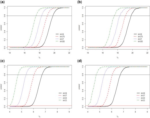
Power curves for different |$\theta$| under two sets of Poisson distribution parameter values (1) |$\lambda_R=21$|, |$\lambda_P=7$| (top row) and (2) |$\lambda_R=7$|, |$\lambda_P=1$| (bottom row). (a and c, left column) for Frequentist approach, while (b and d, right column) for exact Bayesian conjugate prior.
6. Application
This shows that the Bayesian decision rule remains unchanged as in the previous case. We use |$p^{*}=0.975$| to determine NI of GA over sc-IFN beta-1a.
From Table 1, we observe that after 12 months |$37/50$||$\left(74\%\right)$| of the patients who did not receive any therapy developed |${\geq}1$| new CLs counts, |$12/46$||$\left(26\%\right)$| patients treated with sc-IFN beta-1a and |$24/48$||$\left(50\%\right)$| treated with GA respectively developed at least one lesian count. These figures after 24 months came out as |$41/50$||$\left(82\%\right)$| for the patients with no therapy, |$24/46\left(52\%\right)$| for those treated with sc-IFN beta-1a, and |$30/48\left(62\%\right)$| for the GA-treated patients. So, we observe that the percentages of at least one lesian count increased from 1 year to 2 years for all treatment arms. Also, the calculated rates of occurrence of the CLs for no therapy, reference, and test drug, are respectively, 1.53, 0.37, and 0.79 after 1-year and 2.94, 0.72, and 1.29 after 2 years. The rate of the untreated (placebo) group is much higher than those of the treated groups, which indicates that the treatments have beneficial effect in lowering the new CLs development. We first carry out the analysis under the Frequentist approach and calculate the |$p$|-value for testing the hypothesis in equation (6.1) as p-value |$=P_{H_0}(W\,{<}\,W_{\rm obs}), $| where |$W$| is the test statistic given by |$ W=(\hat{\lambda}_{E}-\theta \hat{\lambda}_{R}-\left(1-\theta\right)\hat{\lambda}_{P}|\hat{\lambda}_{P}\,{>}\,\hat{\lambda}_{R}) $| and |$W_{\rm obs}$| is the observed value of |$W$|. The |$p$|-value is then compared with |$\alpha=0.025$| to deduce the Frequentist decision of NI. For Bayesian conjugate prior, we carry out the analysis assuming both non-informative and informative priors. For the non-informative case, we assume Jeffreys prior as |$\text{Gamma}\left(0.5,0.00001\right)$| for |$\lambda_{l}$|, |$l\in\left\{ E,R,P\right\} $| and generate posterior samplers for the three rates from |$ \text{Gamma} $| distributions as in Step 3 of simulation studies, but keeping samples satisfying |$\lambda_{P}\,{>}\,\lambda_{R}$| to account for the AS condition. We calculate the posterior probability for the rejection of |$H_{1}$| as given in the left hand side of (6.2). We report |$P(H_{1}|\text{Data})$| in Table 4 for different values of |$\theta$| in the range |$[0.5,1)$|, in order to ensure that the test drug has a meaningful effect. These posterior probabilities are compared with |$p^{*}$| to deduce the Bayesian decision. In Table 4, we also report the decisions: 1 (if NI is claimed) or 0 (otherwise) for Frequentist as well as Bayesian analyses.
Bayesian and Frequentist decision in the lesian count data where “1” stands for the rejection and “0” stands for acceptance of the null hypothesis. Also posterior probabilities are reported under different priors.
| Posterior probabilities | Decision | ||||||||
|---|---|---|---|---|---|---|---|---|---|
| Conjugate | Non-conjugate | Conjugate | Non-conjugate | ||||||
| |$\theta$| | Non-informative | Informative | Non-informative | Informative | Frequentist decision | Non-informative | Informative | Non-informative | Informative |
| 1-year data | |||||||||
| 0.80 | 0.102 | 0.717 | 0.220 | 0.152 | 0 | 0 | 0 | 0 | 0 |
| 0.75 | 0.198 | 0.786 | 0.275 | 0.220 | 0 | 0 | 0 | 0 | 0 |
| 0.70 | 0.322 | 0.859 | 0.310 | 0.291 | 0 | 0 | 0 | 0 | 0 |
| 0.65 | 0.461 | 0.925 | 0.350 | 0.398 | 0 | 0 | 0 | 0 | 0 |
| 0.60 | 0.590 | 0.957 | 0.384 | 0.615 | 0 | 0 | 0 | 0 | 0 |
| 0.55 | .00717 | 0.976 | 0.413 | 0.845 | 0 | 0 | 1 | 0 | 0 |
| 0.50 | 0.829 | 0.988 | 0.445 | 0.976 | 0 | 0 | 1 | 0 | 1 |
| 2-year data | |||||||||
| 0.80 | 0.262 | 0.226 | 0.266 | 0.280 | 0 | 0 | 0 | 0 | 0 |
| 0.75 | 0.481 | 0.456 | 0.302 | 0.456 | 0 | 0 | 0 | 0 | 0 |
| 0.70 | 0.705 | 0.729 | 0.336 | 0.650 | 0 | 0 | 0 | 0 | 0 |
| 0.65 | 0.847 | 0.902 | 0.355 | 0.821 | 0 | 0 | 0 | 0 | 0 |
| 0.60 | 0.930 | 0.979 | 0.381 | 0.913 | 0 | 0 | 1 | 0 | 0 |
| 0.55 | 0.983 | 0.998 | 0.404 | 0.963 | 1 | 1 | 1 | 0 | 0 |
| 0.50 | 0.994 | 0.999 | 0.431 | 0.990 | 1 | 1 | 1 | 0 | 1 |
From Table 4, we observe that the posterior probabilities increase as the values of |$\theta$| decrease implying higher chance of declaring NI for smaller values of |$\theta$|. For the 1-year data, under Jeffreys prior, we see that the average posterior probability |$P(H_{1}|\text{Data})$| are small for all values of |$\theta$| meaning that NI of GA cannot be claimed for |$\theta\in[0.5,0.8].$| This is due to the fact that the rate of lesion count occurrence for GA-treated patients is higher than those treated with sc-IFN beta-1a, which gives an indication that GA is possibly inferior to sc-IFN beta-1a since its effect is not within the NI margin. But if we choose an informative prior with suitable parameters, then NI can be claimed for |$\theta\leq0.55$|. In this case, we chose the following priors for the three arms respectively: |$E$|: |$\text{Gamma}(8,10)$|, |$R$|: |$\text{Gamma}(20,5)$|, and |$P$|: |$\text{Gamma}(12,8)$|. For the 2-year data also, the rate of lesian count for GA is higher than that of the reference group; however, the difference between the rates is within the NI margin |$\delta$|, to claim NI of GA for small values of |$\theta$|, even under the Jeffreys prior. Considering informative prior, we can still improve on the posterior probabilities. Choosing the following priors: |$E$|: |$\text{Gamma}(64,49.6)$|, |$R$|: |$\text{Gamma}(12,17)$|, |$P$|: |$\text{Gamma}(60,20.4)$|, NI is claimed for |$\theta\leq0.6$|. Finally, considering the non-conjugate prior, for the reformulated hypothesis in (6.1), we assume the following: |$ u_{1} ={\lambda_{R}}/{\lambda_{P}}\sim \text{Beta}(a,b)\mbox{,} u_{2} =\lambda_{P}\sim \text{Gamma}(p,r), $| where |$0\,{<}\,u_{1}\,{<}\,1$|, which satisfies the AS condition (|$\lambda_{R}\,{>}\,\lambda_{P}$|) and |$u_{2}\,{>}\,0$|. For the 1-year data, assuming a relatively non-informative prior: |$\text{Gamma}\left(0.8,1\right)$| for |$E$|; |$\text{Gamma}\left(1.5,1\right)$| for |$P$|; and |$\text{Beta}\left(1,3.1\right)$| for |${\lambda_{R}}/{\lambda_{P}}$|; we observe that NI cannot be claimed for any |$\theta\in[0.5,0.8]$|. However, if the following priors are chosen: |$\text{Gamma}\left(160,200\right)$| for |$E$|; |$\text{Gamma}\left(600,400\right)$| for |$P$|; and |$\text{Beta}\left(200,630\right)$| for |${\lambda_{R}}/{\lambda_{P}}$|; then NI can be claimed for |$\theta=0.5$|. Also for the 2-year data, the observations are similar for the non-informative prior in the non-conjugate setting. NI cannot be claimed for the priors: |$\text{Gamma}\left(0.8,0.62\right)$| for |$E$|; |$\text{Gamma}\left(0.75,0.255\right)$| for |$P$|; and |$\text{Beta}\left(1.2,3.7\right)$| from the ratio |${\lambda_{R}}/{\lambda_{P}}$|. However, for the relatively informative priors: |$\text{Gamma}\left(80,62\right)$| for |$E$|; |$\text{Gamma}\left(75,25.5\right)$| for |$P$|; and |$\text{Beta}\left(12,37\right)$| for |$\frac{\lambda_{R}}{\lambda_{P}}$|; NI can be claimed for |$\theta=0.5$|. We note that the hyper-parameters for both conjugate and non-conjugate priors are so chosen that the mean of the |$ \text{Gamma} $| distribution equals the estimated count rate in the respective arms. Also, we observed that for the 1-year data, more informative priors are needed to claim NI, as compared to the 2-year data. This indicates that the present trial data for 1-year end-point does not support NI strongly, while for 2-year endpoint, NI can be claimed if we choose |$\theta \,{<}\, 0.6$|.
7. Discussion
According to several guidelines, the NI margin should be pre-specified in the protocol, while some allows flexibility of pre-specifying a fixed amount of effect retention (e.g., FDA, 2016; ICH Steering Committee, 1998, 2000; EMA, 2005; Wangge and others, 2013). Thus the value of the NI margin can vary greatly depending on the estimated effect size of the reference treatment (|$\lambda_{R}-\lambda_{P}$|). In this article, we presented novel Frequentist and Bayesian test procedures for three-arm NI trial under fraction margin approach. We proposed more powerful conditional test (Lemma 2.2.2) based on Frequentist principle which directly incorporates the AS condition in NI testing. We believe this is a better usage of available information. Under AS assumption, conditional principle is more realistic and more powerful than the traditional marginal NI testing and it does not result in a biased test (e.g., joint testing of NI and AS). In the conditional Frequentist approach, we conditioned the NI test statistic on |$\hat{\lambda}_R \,{>}\, \hat{\lambda}_P$|; however, it is very much possible to condition it based on the AS test statistic. However, this is not done in the current paper as that will make Bayesian (conditioned on |$ \lambda_R\,{>}\, \lambda_P $|) and Frequentist approach incomparable, since then each approach will use slightly different conditioning statement. In the Bayesian context, we explored conjugate prior and also specified more flexible non-conjugate prior choices. In Section 4.2, for integer-valued parameters we have also shown an interesting connection between Bayesian posterior probability to Frequentist exact probability. This could be further exploited to connect Bayesian and Frequentist sample size in the line of Zaslavsky (2013). Since Bayesian power calculation requires additional computation, we tabulated the sample size in Table 2 under three different types of allocation. We hope that the clinicians will find this readily useful in designing such NI trial.
We have observed that the Bayesian normal approximation and the exact Bayesian approach yield greater power and hence require smaller sample size compared to the Frequentist approach. Albeit, we would like caution an user about the control of type-I error in Bayesian context as pointed out in recent papers by Kopp-Schneider and others (2019) and Psioda and Ibrahim (2018). It is reported that with informative prior strict type-I error control in the Frequentist sense is not possible under Bayesian setup. In this article, all reported type-I errors are “average type-I error” as defined in Gravestock and others (2017), which is essentially an average over all possible outcomes under null distribution. We thank an anonymous reviewer for pointing this out. Also, it is evident that an unbalanced allocation of the sample size in NI trial results in the reduction of the required number of patients to achieve a certain power. According to Pigeot and others (2003), an unbalanced allocation of the total sample size in a NI trial is desirable from ethical and substantial point of view. We also applied our proposed Bayesian test procedure on a clinical trial data on MS. The results suggest that the Bayesian methods perform favorably in all situations and that these methods do not depend on any asymptotic approximation as the Frequentist method.
Notably, with Poisson distributed outcomes, rate/count difference is not the only function of interest. In the binary context, apart from risk difference similar methods for risk ratio and odds ratio has been developed in both Frequentist (Chowdhury and others, 2018b) and Bayesian context Chowdhury and others (2018a) very recently. In a similar line one may frame two-arm NI trial using the ratio of Poisson rates as done in Stucke and Kieser (2013) for two-arm trial. However, for a three-arm trial, defining such a functional (in ratio form) is non-trivial. We are currently developing both the Frequentist and Bayesian methods for these types of functionals. Also for the count type outcome over-dispersion (and under-dispersion) is a frequent issue and Poisson model is not an ideal choice. However, given the dearth of Bayesian article for count data, we did not consider those issues in the current paper. One could use negative binomial (Mütze and others, 2016) or generalized Poisson distribution instead, however the resulting Bayesian (and Frequentist) procedure will be much more involved and as a result left as a future work.
Software
The open source R codes for all the simulation studies and real data analyses performed in this manuscript are available at https://github.com/erina633/Poisson3armNI. Also, there is a README.md file which describes the contents of the R files and all the source functions. All the proofs and additional results are placed in Supplementary Appendix available at Biostatistics online.
Supplementary material
Supplementary material is available at http://biostatistics.oxfordjournals.org.
Acknowledgments
Conflict of Interest: None declared. The article reflects the views of the author and should not be construed to represent FDA’s views or policies.
Funding
The research of first author is partly supported by PCORI (contract number ME-1409-21410); and NIH (P30-ES020957).
References
EMA (
FDA (
