


Summary
Many clinical trials have been conducted to compare right-censored survival outcomes between interventions. Such comparisons are typically made on the basis of the entire group receiving one intervention versus the others. In order to identify subgroups for which the preferential treatment may differ from the overall group, we propose the depth importance in precision medicine (DIPM) method for such data within the precision medicine framework. The approach first modifies the split criteria of the traditional classification tree to fit the precision medicine setting. Then, a random forest of trees is constructed at each node. The forest is used to calculate depth variable importance scores for each candidate split variable. The variable with the highest score is identified as the best variable to split the node. The importance score is a flexible and simply constructed measure that makes use of the observation that more important variables tend to be selected closer to the root nodes of trees. The DIPM method is primarily designed for the analysis of clinical data with two treatment groups. We also present the extension to the case of more than two treatment groups. We use simulation studies to demonstrate the accuracy of our method and provide the results of applications to two real-world data sets. In the case of one data set, the DIPM method outperforms an existing method, and a primary motivation of this article is the ability of the DIPM method to address the shortcomings of this existing method. Altogether, the DIPM method yields promising results that demonstrate its capacity to guide personalized treatment decisions in cases with right-censored survival outcomes.
1. Introduction
In the past decade, there has been a shift towards implementing precision medicine as a more modern approach to defining disease and treating patients (Ashley, 2016). Precision medicine is an approach that tailors treatments to patients at an individualized level in contrast to broadly focusing on average effects. The idea is to better deliver the “right drug at the right dose at the right time to the right patient” (Hamburg and Collins, 2010; Collins and Varmus, 2015). Overall, the primary goal is to improve individual patient outcomes by being more precise about how and what treatments are recommended.
In order to achieve the goals of precision medicine, it is important to identify specific subgroups that perform either especially well or especially poorly with a given treatment. Prominent examples of success include the identification of trastuzumab as a better drug for patients with breast tumors that overexpress the HER-2 protein (Romond and others, 2005). Another example is the identification of imatinib as a better treatment for chronic-phase chronic myeloid leukemia patients who are positive for the Philadelphia chromosome (O’Brien and others, 2003). Though there have been successes in the recent past, there are still opportunities for new discoveries in oncology and beyond.
Continuing to discover clinically relevant subgroups may be improved with novel biostatistical methods. Motivated by the importance score proposed in the work by Chen and others (2007), as well as the tree-based methodology developed by Zhu and others (2017), we propose the depth importance in precision medicine (DIPM) method. This method is a classification tree designed to identify clinically meaningful subgroups in the precision medicine setting. More specifically, the method mines existing clinical data by systematically searching through available covariates to determine whether there are any subgroups that exhibit particularly favorable performance with a given treatment. Within the tree structure, the DIPM method utilizes a depth variable importance score to select the “best" candidate variable to split each node. Previously in the literature, this variable importance measure has been used to assess the importance of variables after a random forest is fit (Chen and others, 2007; Zhang and Singer, 2010). The DIPM method diverges from the original usage of the variable importance measure by using it within a tree and within the precision medicine framework.
In previous work, we have already developed the DIPM method for the identification of clinically meaningful subgroups for data sets with continuous outcome variables and binary treatments. Here, we present the DIPM method for the analysis of clinical data with right-censored survival outcomes. Survival outcomes are commonly collected in clinical trials and measure the time to an event of interest. Examples of events of interest include tumor recurrence, disease relapse, and death. Furthermore, survival data present additional challenges due to subjects who do not experience the event of interest by the end of study as well as subjects who are lost to follow-up, i.e., subjects who are right-censored. The proposed method is designed to account for right-censored observations within the framework of precision medicine.
However, the idea of combining precision medicine with the classification tree structure is not novel. There are several existing classification tree methods designed for the analysis of survival data in this setting. Existing methods designed for the analysis of survival data include extensions of the following: the RECursive Partition and Amalgamation (RECPAM) algorithm (Negassa and others, 2005), model-based partitioning (MOB) (Zeileis and others, 2008; Seibold and others, 2016), interaction trees (IT) (Su and others, 2008), subgroup identification based on differential effect search (SIDES) (Lipkovich and others, 2011), generalized, unbiased, interaction detection, and estimation (GUIDE) trees (Loh and others, 2015), and the weighted classification tree method developed by Zhu and others (2017). Despite the existence of these methods, we aim to further improve upon the performance of these methods in terms of computation and ability to identify clinically meaningful subgroups. Our key idea is to construct a variable importance score that addresses the blind spots of the weighted misclassification variable importance score of the method by Zhu and others (2017). For this reason, we focus on comparing our method to theirs. As a whole, empirical evidence supports that our method is superior to theirs due to its greater accuracy, consideration of a broader pool of candidate splits, and overall relative simplicity. The remainder of this article is structured as follows. First, details of the proposed method are described. Second, a literature review is provided to further discuss existing tree-based methods for precision medicine. Next, simulation scenarios assessing the performance of the proposed method are explored. Then, results of applications to two real-world data sets are presented. Lastly, the discussion section includes concluding remarks and directions for future work.
2. Method
2.1. Overview
The proposed method is designed for the analysis of data sets with right-censored time-to-event survival outcomes |$Y$|, censoring indicator |$C$|, and two possible treatment assignments |$A$| and |$B$|. When |$C=1$|, this indicates that the event of interest has occurred. Meanwhile, |$C=0$| indicates that an observation is right-censored. Candidate split variables are also part of the data, and the candidate variables may be binary, ordinal, or nominal. All of the learning data are said to be in the first or root node of the classification tree, and nodes may be split into two child nodes. Borrowing the terminology used in Zhu and others (2017), at each node in the tree, a random forest of “embedded" trees is grown to determine the best variable to split the node. Once the best variable is identified, the best split of the best variable is the split that maximizes the difference in response rates between treatments |$A$| and |$B$|. Note that “the best variable" is “best" in a narrow sense as defined below. In addition, a flowchart outlining the general steps of the DIPM algorithm is provided in Figure 1.
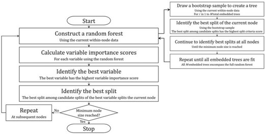
Overview of DIPM method classification tree algorithm. A flowchart outlining the general steps of the proposed method’s algorithm is depicted in the figure above.
2.2. Depth variable importance score
The depth variable importance score is used to find the best split variable at a node. In general, the depth variable importance score incorporates two pieces of information: the depth of a node within a tree and the magnitude of the relevant effect. The reasoning behind using depth information is that more important variables tend to be selected closer to the root node of a tree. Meanwhile, the strength of a split is also taken into account. This second component of the variable importance score is a statistic that is specified depending on the context of the given analysis.
Next, a “|$G$| replacement” feature is implemented that potentially alters the variable importance scores |${score}(T,j)$|. For each tree |$T$| in the forest, the |$G$| at each split is replaced with the highest |$G$| value of any of its descendant nodes if this maximum exceeds the value at the current split. This replacement step is performed because a variable that yields a split with a large effect of interest further down in the tree is still important even if its importance is not captured right away. By “looking ahead” at the |$G$| values of future splits, a variable’s importance is reinforced.
The best split variable is the variable with the largest value of |${score}(f,j)$|.
2.3. Split criteria
The best split is the split with the largest |$z^2$| Wald test statistic that tests the significance of |$\beta_3$| in the Cox model (2.2). Among the list of candidate splits, only splits with child nodes with at least |$nmin$| subjects are considered. At a given node, splitting stops when there are less than |$nmin$| subjects in the child nodes of every candidate split.
2.4. Random forest
A random forest is grown at each node in the overall tree and then used to select the best split variable. Once this variable is identified, all possible splits of the variable are considered, and the best split is found using the criteria described in Section 2.3.
The forest is constructed as follows. The forest contains a total of |$M$| embedded trees. Each embedded tree is grown using a bootstrap sample. The bootstrap sample contains 80% of the number of subjects in the current node, and data are randomly sampled without replacement. Then, at each node in the embedded trees, all possible splits of all of the variables are considered. The best split is again found using the criteria described in Section 2.3.
The recommended value of |$M$| total embedded trees is 1000. However, in order to reduce computation time, the smaller recommended value of |$M$| is |$\min{(\max{(\sqrt{n}, \sqrt{p})}, 1000)}$|. |$n$| is the total sample size, and |$p$| is the total number of candidate split variables in the data. These specifications of |$M$| reduce the computation time of the method while still having enough embedded trees to maintain accuracy.
Also, note that the minimum number of subjects in nodes of the overall classification tree does not have to equal the minimum number of subjects in nodes of the embedded trees. Put another way, |$nmin$| is the minimum node size of the overall tree, while |$nmin2$| is the minimum node size of trees in the random forest. |$nmin$| and |$nmin2$| do not have to be equivalent.
2.5. Best predicted treatment class
The best predicted treatment class of a node is the treatment group that performs best based on the subjects within the given node. Here, the best predicted treatment class is determined by comparing the mean survival times of each treatment group. These means may be estimated by calculating the area under the Kaplan–Meier curve of each treatment group.
|$\hat{\mu}_A=\int_0^{\tau_A} \hat{S}_A (t) {\rm d}t$| is the estimated mean survival time of treatment group |$A$|, and |$\hat{\mu}_B=\int_0^{\tau_B} \hat{S}_B (t) {\rm d}t$| is the estimated mean survival time of treatment group |$B$|. Each value of |$\tau$| is set equal to the largest observed time in the respective treatment group. Klein and Moeschberger (2003) describe two options for defining |$\tau$| when the largest observed time is censored. One option is to convert the largest observed time to an event. The second option is to use the longest possible time that a subject could survive as determined by the investigator. Here, we use the first option.
Larger areas, i.e., larger mean survival estimates, denote better survival rates when the event of interest is negative. Defining negative events tends to be more common than defining positive events of interest. Therefore, if |$\hat{\mu}_A > \hat{\mu}_B$|, then treatment |$A$| is the best predicted treatment at the node. If |$\hat{\mu}_B > \hat{\mu}_A$|, then treatment |$B$| is the best predicted treatment. If |$\hat{\mu}_A = \hat{\mu}_B$|, then neither treatment is best.
2.6. Extension to multiple treatments
The random forest is constructed in the same way as described in Section 2.4. The only difference is that the split criteria used is the largest |$z^2$| Wald test statistic that tests the significance of the most significant split by treatment interaction term in the Cox model (2.4). Note that these split criteria are used within the random forest as well as after the best split variable is identified in order to find the best split of the variable. Finally, the best predicted treatment class of a node is the treatment group with the largest mean survival time at the node.
2.7. Implementation
The proposed method is implemented using R. The R code calls a C program to generate the final classification tree. The C backend is used to take advantage of C’s higher computational speed in comparison to R. All of the simulation studies and data analyses are implemented in R. The software implementation of our method and simulated data examples are currently available on GitHub (https://github.com/chenvict/dipm).
3. Existing methods
As mentioned in the introduction, there are multiple existing tree-based methods designed for the analysis of data with right-censored survival outcomes in this research area. Several of these methods rely on models to identify subgroups relevant to precision medicine. For instance, in the RECPAM algorithm developed by Negassa and others (2005) and the IT method developed by Su and others (2008), the split criteria are based on Cox proportional hazards models that contain interaction terms with the treatment variable. Meanwhile, Loh and others (2015) extend their GUIDE method to the analysis of survival data by using Poisson regression to fit proportional hazards models. They use this approach so that there is a common estimated baseline cumulative hazard function across nodes instead of having different baseline cumulative hazard functions from separate proportional hazards models in each node. In the MOB method developed by Zeileis and others (2008), it is assumed that each subgroup has its own optimal model, where the model is a model of the user’s choice. Parameter estimates of the model are fit by minimizing an objective function that is usually the negative log-likelihood, and nodes are split with the split that locally optimizes the objective function in the two child nodes. This method accommodates survival data when the selected model is a Weibull or Cox model.
The SIDES method by Lipkovich and others (2011) analyzes data with binary treatment variables, where one treatment is labeled the reference treatment and the other the alternative treatment. SIDES only considers subgroups where the alternative treatment does better than the reference. SIDES identifies multiple subgroups, and the final subgroups may be overlapping (i.e., some subjects may be members of more than one subgroup). In addition, within a candidate search, once a covariate has already been used to define a subgroup, the covariate is no longer considered for future splits. The split criteria are based on p-values from |$Z$| statistics for testing one-sided hypotheses for treatment efficacy in the subgroups. Also, the SIDES method aims to be both confirmatory and exploratory.
Zhu and others (2017) propose a weighted classification tree method designed to perform well with high-dimensional covariates. Improving upon the limitations of this method is one of the primary motivations behind the development of our DIPM method. In the weighted classification tree method, subject specific weights are first calculated for each subject. Similarly to our DIPM method, their method also constructs a random forest of embedded trees at each node. However, their forest of embedded trees consists of extremely randomized trees. At each node of these embedded trees, one split is randomly selected from each candidate split variable, and these randomly selected splits make up the pool of candidate splits. Then, once the forest of embedded trees is constructed, the out-of-bag samples at each node of the overall tree are used in their variable importance score to find the best split variable of the current node. Their importance score is a ratio of misclassified treatment classification when the values of a variable are randomly permuted versus left the same. The method is extended to analyzing survival data with double weighted trees, where the second set of weights are the Kaplan–Meier weights.
4. Simulation studies
4.1. Methods
In each simulation scenario, two methods are compared to the proposed DIPM method. The first is the weighted classification tree method developed by Zhu and others (2017), since a primary motivation for the DIPM method is to address the limitations of their existing method. The second comparison method is a tree method that does not contain random forests of embedded trees. Instead, nodes are split using the best split among all possible splits of all candidate split variables in the data. The split criteria is the Cox split value described in Section 2.3. Note that this additional method is “novel" in the sense that we have built and implemented the method ourselves. However, the general structure of this method is equivalent to the traditional classification tree approach and can therefore be considered a simple and obvious choice.
For the DIPM method, the value of |$M$| total embedded trees used in all of the simulation scenarios is the value recommended in Section 2.4: |$\min{(\max{(\sqrt{n}, \sqrt{p})}, 1000)}$|. |$n$| is the total sample size, and |$p$| is the total number of candidate split variables. The value of |$M$| embedded trees used for the weighted method is 1000. Finally, for the simple Cox splits tree, since this method does not contain random forests of embedded trees, there is no applicable value of |$M$|.
4.2. Scenarios
The following scenarios assess the proposed DIPM method and compare it to the weighted classification tree and simple Cox splits method. The overall strategy is to design scenarios with known, underlying signals and measure how often each method accurately detects these signals. In all simulations, treatment assignments are randomly generated from |$\{A, B\}$| with equal probability. |$I_A$| and |$I_B$| denote the indicators for assignments to treatments |$A$| and |$B,$| respectively. In all eight scenarios, |$\epsilon=0.8N_1 + 0.5N_2+0.3U_1+0.4U_2$|, where |$N_1$| and |$N_2$| are independent and normally distributed, i.e., N(0, 1), and |$U_1$| and |$U_2$| are independent and uniform, i.e., Uniform(0, 1).
In the first five scenarios, the accuracy of each method is assessed as the total number of variables increases and as the sample size of the data increases. To be specific, we compare method performance when there are 20 candidate split variables in the data versus 50 candidate split variables while simultaneously observing the differences between having a sample size of 250 versus 500. In general, we expect method performance to decrease as the number of candidate split variables increases because the probability of missing truly important signals by chance tends to increase when there are more variables and splits to choose from. In regard to sample size, we expect method performance to increase with larger sample sizes because a larger sample size provides more information about the underlying model.
When there are 20 candidate split variables in the data, the first 8 variables are ordinal and normally distributed, i.e., |$N(0,1)$| rounded to the fourth decimal place. The next 7 are nominal and sampled from the Discrete Uniform distribution, i.e., Discrete Uniform[1, 5]. The remaining 5 variables are binary, i.e., Discrete Uniform[0, 1]. When there are 50 candidate split variables in the data, the three variable types are sampled from the same distributions, respectively. However, instead, there are 18 ordinal variables, 17 nominal variables, and 15 binary variables. For each situation and scenario, 500 simulations are run.
Scenario 1: The first scenario consists of an exponential survival time model containing the treatment and one important continuous variable. |$Y_0 \sim Exp(e^\mu)$|, |$C \sim Exp(e^{0.3(U_1+U_2)})$|, |$Y = \min(Y_0, C)$|, and the censoring rate is 55%. The formula for |$\mu$| is:
Scenario 2: The second scenario consists of a Weibull survival time model containing the treatment and one important continuous variable. |$Y_0 \sim {\rm Weibull}$|(scale parameter = |$e^{\mu}$|, shape parameter = 2), |$C \sim {\rm Exp}(e^{-0.3(U_1+U_2)})$|, |$Y = \min(Y_0, C)$|, and the censoring rate is 49%. The formula for |$\mu$| is:
Scenario 3: The third scenario consists of an underlying tree model containing the treatment and one important binary variable. |$Y_0 \sim {\rm Weibull}$|(scale parameter = |$e^{\mu}$|, shape parameter = 2), |$C \sim {\rm Exp}(0.8 e^{-\mu})$|, |$Y = \min(Y_0, C)$|, and the censoring rate is 48%. The formula for |$\mu$| is:
Scenario 4: The fourth scenario consists of an underlying tree model containing the treatment and three important binary variables. |$Y_0 \sim {\rm Weibull}$|(scale parameter = |$e^{\mu}$|, shape parameter = 2), |$C \sim {\rm Exp}(0.8 e^{-\mu})$|, |$Y = \min(Y_0, C)$|, and the censoring rate is 48%. The formula for |$\mu$| is:
Scenario 5: The fifth scenario consists of an underlying model where the proportional hazards assumption is violated. The model is a Weibull survival time model that differs by treatment group and contains one important continuous variable. |$Y_0 \sim {\rm Weibull}$|(scale parameter = 1, shape parameter = |$e^{\mu}$|), |$C \sim {\rm Exp}(e^{-0.3(U_1+U_2)})$|, |$Y = \min(Y_0, C)$|, and the censoring rate is 68%. When treatment = 0, the formula for |$\mu$| is:
When treatment = 1, the formula for |$\mu$| is:
In the next four scenarios, 1, 10, and 100 |$Z$| variables correlated with a truly important variable |$X_1$| are added to the data. There are a number of |$X$| variables in the data that are all ordinal and normally distributed, i.e., X|$\sim N(0, \Sigma)$| and |$\Sigma_{i,j}=\rho^{|i-j|}$|, where |$\rho=0.25$|. Note that these |$X$| values are also used in the simulation scenarios by Zhu and others (2017). For scenarios 6 through 8, |$Z = 0.8X_1 + 0.1N_1 + 0.1N_2 + N_3$|, where |$N_1$| and |$N_2$| are both N(0, 1), and |$N_3$| is N(0, sd=0.2). For scenario 9, |$Z = 0.8X_1 + 0.1X_2 + 0.1X_3 + N_4$|, where |$N_4$| is N(0, SD = 0.4). For each number of added |$Z$| variables, 500 simulations are run for sample sizes of 300.
Scenario 6: The sixth scenario consists of an exponential survival time model containing the treatment and one important continuous variable. Overall, this scenario contains one |$X$| variable and increasing numbers of |$Z$| variables as described above. |$Y_0 \sim {\rm Exp}(e^\mu)$|, |$C \sim {\rm Exp}(e^{0.3(U_1+U_2)})$|, |$Y = \min(Y_0, C)$|, and the censoring rate is 51%. The formula for |$\mu$| is:
Scenario 7: The seventh scenario consists of a Weibull survival time model containing the treatment and one important continuous variable. Overall, this scenario contains one |$X$| variable and increasing numbers of |$Z$| variables as described above. |$Y_0 \sim {\rm Weibull}$|(scale parameter = |$e^{\mu}$|, shape parameter = 2), |$C \sim {\rm Exp}(e^{-0.3(U_1+U_2)})$|, |$Y = \min(Y_0, C)$|, and the censoring rate is 53%. The formula for |$\mu$| is:
Scenario 8: The eighth scenario consists of an underlying tree model containing the treatment and one important binary variable. Overall, this scenario contains one |$X$| variable and increasing numbers of |$Z$| variables as described above. |$Y_0 \sim {\rm Weibull}$|(scale parameter = |$e^{\mu}$|, shape parameter = 2), |$C \sim {\rm Exp}(0.8 e^{-\mu})$|, |$Y = \min(Y_0, C)$|, and the censoring rate is 48%. The formula for |$\mu$| is:
Scenario 9: The ninth scenario consists of an underlying tree model containing the treatment and three important binary variables. Overall, this scenario contains three |$X$| variables and increasing numbers of |$Z$| variables as described above. |$Y_0 \sim {\rm Weibull}$|(scale parameter = |$e^{\mu}$|, shape parameter = 2), |$C \sim {\rm Exp}(0.8 e^{-\mu})$|, |$Y = \min(Y_0, C)$|, and the censoring rate is 48%. The formula for |$\mu$| is:
4.3. Results
As mentioned in Section 4.2, the overall strategy of all of the simulations is to design scenarios with known, underlying signals to assess how well each method accurately detects these signals. Accuracy is measured by calculating the proportion of correct variable selection among the total number of simulation runs in each setting. The first set of scenarios examines how each method performs as the total number of candidate split variables increases and as the total sample size increases. In general, performance is expected to decrease as the total number of candidate split variables increases, and performance is expected to increase as the total sample size increases. Meanwhile, the second set of scenarios examines how each method performs as the number of candidate split variables correlated with a truly important variable increases. In general, performance is expected to decrease as the number of correlated variables increases. Despite these general expectations, overall, the simulations are designed to compare how each method performs relative to one another.
All of the simulation results are presented in Table 1. For the first set of scenarios numbered 1 through 5, as expected, all methods perform worse as the number of candidate split variables increases, and all methods perform better as the sample size increases. In almost every scenario and situation, the DIPM method outperforms the other two methods. Between the simple Cox tree and the weighted method, the simple Cox tree tends to outperform the weighted method as well. One exception to this pattern is with the simple tree model of depth 2 in scenario 3. When the sample size is 500 and there are 20 candidate split variables in the data, the weighted method does slightly better than the other two methods. The other exception occurs in the fourth scenario which has an underlying tree model of depth 3. In scenario 4, when the sample size is 250, the weighted method again performs worst. However, when the sample size increases to 500, the weighted method outperforms the DIPM method and the simple Cox tree. In these specific situations, the weighted method gains an extra advantage from having more available information with the larger sample size. However, this pattern is not robust enough to also occur in the other simulation settings.
Results of simulation scenarios. Proportions of 500 simulation runs in which |$X_1$| is correctly selected at the first split in scenarios 1–3 and 5–8 and |$X_1$| then |$X_2$| and |$X_3$| are correctly selected as the first three splits in scenarios 4 and 9. |$n$| is the total sample size, and |$p$| denotes the total number of candidate split variables. In scenarios 6–9, the sample size is 300.
| |$n=250$| | |$n=500$| | ||||
|---|---|---|---|---|---|
| Scenario | Method | |$p=20$| | |$p=50$| | |$p=20$| | |$p=50$| |
| Weighted | 0.076 | 0.040 | 0.136 | 0.080 | |
| 1. Non-tree, exponential | Simple | 0.422 | 0.262 | 0.586 | 0.466 |
| DIPM | 0.446 | 0.290 | 0.600 | 0.476 | |
| Weighted | 0.116 | 0.066 | 0.192 | 0.076 | |
| 2. Non-tree, Weibull | Simple | 0.560 | 0.432 | 0.724 | 0.664 |
| DIPM | 0.566 | 0.444 | 0.750 | 0.682 | |
| Weighted | 0.700 | 0.498 | 0.912 | 0.856 | |
| 3. Tree of depth 2 | Simple | 0.732 | 0.650 | 0.910 | 0.874 |
| DIPM | 0.748 | 0.680 | 0.910 | 0.888 | |
| Weighted | 0.740 | 0.638 | 0.950 | 0.946 | |
| 4. Tree of depth 3 | Simple | 0.760 | 0.758 | 0.910 | 0.902 |
| DIPM | 0.784 | 0.784 | 0.942 | 0.918 | |
| Weighted | 0.072 | 0.036 | 0.068 | 0.040 | |
| 5. Non-tree, non-PH | Simple | 0.146 | 0.062 | 0.232 | 0.134 |
| DIPM | 0.156 | 0.066 | 0.242 | 0.124 | |
| No. of Z Vars. | Weighted Method | Simple Cox splits | DIPM Method | ||
| 1 | 0.586 | 0.644 | 0.694 | ||
| 6. Non-tree, exponential | 10 | 0.020 | 0.098 | 0.070 | |
| 100 | 0.000 | 0.004 | 0.002 | ||
| 1 | 0.642 | 0.708 | 0.756 | ||
| 7. Non-tree, Weibull | 10 | 0.026 | 0.130 | 0.110 | |
| 100 | 0.000 | 0.004 | 0.002 | ||
| 1 | 0.930 | 0.994 | 0.994 | ||
| 8. Tree of depth 2 | 10 | 0.616 | 0.970 | 0.962 | |
| 100 | 0.126 | 0.812 | 0.770 | ||
| 1 | 0.634 | 0.636 | 0.656 | ||
| 9. Tree of depth 3 | 10 | 0.092 | 0.302 | 0.270 | |
| 100 | 0.002 | 0.060 | 0.040 | ||
For scenarios 6 through 9, as expected, all methods perform worse with increasing numbers of variables correlated with truly important variable |$X_1$|. The DIPM method and the simple Cox tree both outperform the weighted method across all four of these scenarios. The weighted method appears to be more sensitive to added amounts of correlation. When comparing the DIPM method to the simple Cox tree, the DIPM method tends to perform similarly to the latter method, and in a few instances, performs better. In non-tree scenarios 6 and 7, the DIPM method outperforms the Cox splits tree when there is 1 |$Z$| variable in the data. When there are 10 and 100 |$Z$| variables in the data, the two methods perform similarly. In addition, in tree scenarios 8 and 9, the Cox splits tree slightly outperforms the DIPM method. However, when there is 1 |$Z$| variable in the data, the DIPM method performs either exactly the same or better than the Cox splits tree. In general, because the DIPM method and Cox splits tree consider a broader pool of candidate splits, these methods exhibit superior performance in the presence of correlated variables.
In summary, across different underlying models, the DIPM method tends to outperform the weighted method. This is because in the embedded trees of the DIPM method, a larger pool of candidate splits is considered. By contrast, in the weighted method, each candidate split variable contributes just one randomly selected split to the pool of candidate splits at each node. Though considering fewer splits yields a shorter computation time for the weighted method, this also results in a loss in accuracy as demonstrated by the simulation scenarios here.
5. Applications
5.1. Tamoxifen data
The first data application uses the GSE6532 cohort of microarray data for breast cancer patients (Loi and others, 2007). This data set is available online at the Gene Expression Omnibus (GEO) repository database. The sample contains 277 patients who received the treatment drug tamoxifen and 137 patients in the control group. The outcome variable for these data is time to distant metastasis. The candidate covariates are age, grade of tumor, size of tumor, and 44 928 gene expression measurements.
These data are also analyzed by Zhu and others (2017) using their weighted classification tree method. Following their analysis, the top 500 genes, i.e., the 500 genes with the largest marginal variances, are used in addition to the three clinical variables age, grade of tumor, and size of tumor. For grade of tumor, missing values are set to 0. In total, after removing subjects with missing outcomes, the final data set used for analysis contains 393 subjects and 503 candidate split variables. The censoring rate of these data is 64.63%. Note that this final data set is exactly equivalent to the data set used by Zhu and others (2017) for their published results.
Furthermore, note that in our analysis, we use a maximum tree depth of 3 and a simple pruning strategy in which two terminal sister nodes are pruned if they both have the same optimal treatment assignment. A maximum tree depth of 3 is similar to but less than the recommended “maximum number of covariates defining a subgroup” equal to 3 in the SIDES method by Lipkovich and others (2011). For us, a maximum tree depth of 3 is equal to a maximum of 2 covariates defining a subgroup. Though the two values are not exactly equivalent, both approaches share the same philosophy that less complexity in the identified subgroups tends to be favorable in practice. Also, consider that using a larger maximum number of covariates to define a subgroup yields a greater number of identified subgroups compared to using a smaller number of covariates. Identifying more subgroups within the same data results in subgroups with smaller sample sizes.
The analysis done by Zhu and others (2017) yields a final tree with a single split. The single split uses the gene expression of TSPAN8. For each of their two final subgroups, Zhu and others (2017) present the Kaplan–Meier curves and log-rank test p-values comparing the two treatments. As shown in Figure 2, the low expression subgroup has a p-value slightly greater than 0.05, and the high expression subgroup has a p-value of 0.456.
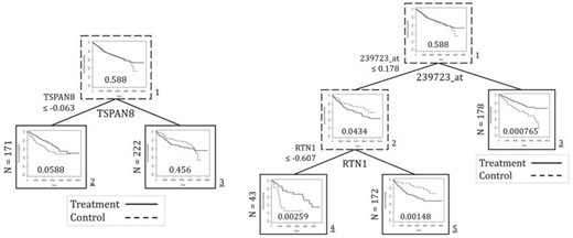
Results of tamoxifen data application. The final tree and corresponding final subgroups from Zhu and others (2017) are presented (left) in addition to the results from the DIPM method (right). The plots depict the Kaplan–Meier curves and log-rank test p-values by treatment group of the data at each node.
Our analysis using the DIPM method identifies the gene expression of 239723_at at the first split and RTN1 at the second split. We examine the Kaplan–Meier curves and log-rank p-values for a tree split with only 239723_at and therefore two final subgroups. We also examine the corresponding values for the tree split with 239723_at and RTN1 and therefore three final subgroups. The results of these trees are also presented in Figure 2.
Interestingly, the two trees yield final subgroups that all have p-values smaller than 0.05, and the subgroups identify different optimal treatments. For the tree split with only 239723_at, the low expression subgroup yields a p-value of 0.0434, and the control arm is the better treatment. The high expression subgroup yields a p-value of 0.000765, and Tamoxifen is better. For the tree split with both 239723_at and RTN1, the low 239723_at and low RTN1 expression subgroup yields a p-value of 0.00259, and the Tamoxifen treatment is better. Meanwhile, the low 239723_at and high RTN1 expression subgroup yields a p-value of 0.00148, and the control arm is better.
In conclusion, the splits identified by the DIPM method appear to be statistically meaningful. Furthermore, these subgroups are more statistically meaningful than the final subgroups identified by Zhu and others (2017). Overall, the proposed method demonstrates practical utility and outperforms an existing method.
5.2. IBCSG data
The second application is a data set from the International Breast Cancer Study Group Trial for premenopausal women with breast cancer and node-positive disease (Group, 1996). The data set contains 1015 patients who were randomized to treatment groups in a |$2 \times 2$| factorial design. Treatments consisted of courses of cyclophosphamide, methotrexate, and fluorouracil (CMF) for 3 or 6 months with or without three single courses of reintroduction CMF. In other words, there are four treatment groups: CMF6, CMF6 + 3 reintroduction CMF, CMF3, and CMF3 + 3 reintroduction CMF. The seven candidate split variables used are: age, number of positive nodes of the tumor, estrogen receptor (ER) status, and the earliest measures of four quality of life indicators: mood, physical well-being, perceived coping, and appetite. The primary outcome is overall survival. The censoring rate of these data is 70.84%.
Due to the |$2\times2$| factorial design of the trial, we can analyze the data in multiple ways. We can collapse treatment groups and consider the effect of duration of treatment alone or the effect of reintroduction of treatment alone. However, with our novel extension for multiple treatments, we may also consider all four treatment groups simultaneously. Therefore, the first comparison studies duration; CMF6 is combined with CMF6 + 3 reintroduction CMF, and CMF3 is combined with CMF3 + 3 reintroduction CMF. Then, the second comparison examines the effects of reintroduction therapy; CMF3 + 3 reintroduction CMF is combined with CMF6 + 3 reintroduction CMF, and CMF3 is combined with CMF6. Lastly, the third comparison compares all four treatment groups at once. When examining the data overall, it appears that in general, longer duration CMF is better, and reintroduction CMF is better than no reintroduction. However, none of these relationships are statistically significant, as the log-rank test p-values by treatment group as defined in the three scenarios above are 0.359, 0.345, and 0.522, respectively.
Among the seven candidate split variables, for all comparisons, the DIPM method selects the quality of life variables in the tree. The results for the duration comparison, reintroduction therapy comparison, and comparing all four treatments at once are shown in Figure 3. We use the Kaplan–Meier curves and log-rank tests by treatment in each analysis. For the duration comparison, we present a tree with three subgroups. The first subgroup with lower appetite and physical well-being scores, i.e., a better clinical health profile based on these scores, does not have a clear optimal treatment assignment (p-value = 0.469). However, the sister node of this subgroup with higher physical well-being scores, i.e., worse physical well-being, identifies the shorter duration CMF3 treatment as optimal (p-value = 0.0305). Meanwhile, the third and final subgroup with the worst health profiles identifies the longer duration CMF6 treatment as optimal (p-value = 0.00452).
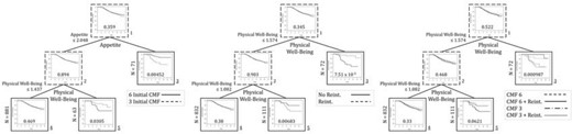
Results of IBCSG data application. The final tree and corresponding subgroups using the DIPM method are presented when studying duration of treatment (left), reintroduction therapy (center), and comparing all four treatments at once (right). The plots depict the Kaplan–Meier curves and log-rank test p-values by treatment factor at each node. Note that lower appetite and physical well-being quality of life scores denote better outcomes.
For the reintroduction therapy comparison, we again present a tree with three final subgroups. The first subgroup has lower physical well-being scores, i.e., better physical well-being, and there is no clear optimal treatment (p-value = 0.38). The sister node of this subgroup has slightly worse physical well-being, and the non-reintroduction therapy is identified as optimal (p-value = 0.00683). The third and final subgroup has the worst physical well-being, and reintroduction therapy is identified as optimal (p-value = 7.51e|$-$|5).
Finally, when comparing all four treatment groups at once, we present a tree yielding three subgroups. Again, all splits utilize physical well-being scores. The first subgroup with lower physical well-being scores, i.e., better physical well-being, once again has no clear optimal treatment (p-value = 0.33). The second subgroup with slightly worse physical well-being identifies the two non-reintroduction therapies CMF3 and CMF6 as optimal treatments (p-value = 0.0621). Lastly, the third subgroup with the worst physical well-being does best with the two reintroduction therapies, and CMF6 + reintroduction is the overall optimal treatment (p-value = 0.000987).
Overall, our results indicate that subjects with worse health profiles at the start of the study have better survival rates in the longer duration CMF and reintroduction therapy groups. It seems that subjects with lower physical well-being to begin with require longer exposure to the treatment. Those with better health profiles potentially benefit from a protective effect, as no optimal treatment is identified. Furthermore, subjects with only slightly worse health profiles experience better survival on the shorter duration and non-reintroduction therapies.
6. Discussion
Based on simulation results and applications to real-world data, the proposed DIPM method for right-censored survival outcomes appears both promising and useful. The proposed method demonstrates satisfactory performance in accurately recovering true feature signals in simulation data and identifies statistically significant subgroups when applied to real-world data. In the case of the tamoxifen gene expression data set, we find that our method identifies subgroups that are more highly statistically significant than the subgroups identified by an existing method. Therefore, in this data application, our method outperforms the existing method.
A noteworthy criticism of forest-based methodology involves the uncertainty in how many trees ought to be used. In Section 2, we recommend using |$\min{(\max{(\sqrt{n}, \sqrt{p})}, 1000)}$| trees, where |$n$| is the total sample size of the data, and |$p$| is the total number of candidate split variables. This value is based on the empirical evaluation of the method’s performance when the number of trees is the square root of |$n$| or |$p$| versus 1000. A reduction in the number of trees is desirable to shorten computation time while still preserving accuracy. Nevertheless, our recommended value may seem too small when |$n$| or |$p$| is large, i.e., greater than 1000. Zhang and Wang (2009) present several approaches for finding the size of the “smallest forest.” One approach is to define a value that captures the overall accuracy of the forest. Then, this value can be calculated upon removal of a single tree. The tree that yields the smallest change in accuracy may be removed from the forest. Perhaps another direction for future work would be the integration of this approach within the DIPM method.
Another topic to consider is computation time. Though the DIPM method is designed to address limitations of the weighted method by Zhu and others (2017), their method requires markedly less time to run. For example, the weighted method requires less than 1 min to generate results for the application in Section 5.1. By contrast, the DIPM method takes 1–2 days. Because the weighted method considers one randomly selected split from each candidate split variable instead of all possible splits, their method is much faster. However, as shown in Section 5.1, the potential tradeoff is a loss in accuracy.
Finally, consider that the purpose of the DIPM method is to identify subgroups using existing clinical data. The DIPM method, in addition to the existing methods described earlier, are more so designed as exploratory rather than confirmatory methods, though one neat way of providing confirmatory information about identified subgroups is the application of the bootstrap calibrated confidence intervals developed by Loh and others (2016). True biological relevance of identified subgroups must be confirmed by clinical experts and further clinical trials. However, the method’s exploratory nature does not negate its potential usefulness. For example, investigators interested in identifying subgroups that have an enhanced treatment effect within a failed trial may use the DIPM method to identify subgroups of interest for future investigation. Though it is expected that most early phase trials will fail, considering the high cost of each trial, it may be worthwhile to explore the data for any information that may be useful later on. Therefore, exploratory tree-based methods such as the DIPM method have useful applications in the realization of precision medicine and clinical trials.
Supplementary material
Supplementary material is available at http://biostatistics.oxfordjournals.org.
Acknowledgments
We thank an Associate Editor and two anonymous reviewers for their helpful comments. The GSE6532 cohort of Tamoxifen treatment data used in this article are obtained from the National Center for Biotechnology Information (NCBI) online Gene Expression Omnibus (GEO) database. They did not participate in the analysis of the data or the writing of this report.
Conflict of Interest: None declared.
Funding
Dr. Zhang’s research is supported in part by the National Institutes of Health (NIH) (R01HG010171 and R01MH116527) and the National Science Foundation (NSF) (DMS1722544).
