


ABSTRACT
A generalized phase 1-2-3 design, Gen 1-2-3, that includes all phases of clinical treatment evaluation is proposed. The design extends and modifies the design of Chapple and Thall (2019), denoted by CT. Both designs begin with a phase 1-2 trial including dose acceptability and optimality criteria, and both select an optimal dose for phase 3. The Gen 1-2-3 design has the following key differences. In stage 1, it uses phase 1-2 criteria to identify a set of candidate doses rather than 1 dose. In stage 2, which is intermediate between phase 1-2 and phase 3, it randomizes additional patients fairly among the candidate doses and an active control treatment arm and uses survival time data from both stage 1 and stage 2 patients to select an optimal dose. It then makes a Go/No Go decision of whether or not to conduct phase 3 based on the predictive probability that the selected optimal dose will provide a specified substantive improvement in survival time over the control. A simulation study shows that the Gen 1-2-3 design has desirable operating characteristics compared to the CT design and 2 conventional designs.
1 INTRODUCTION
Conventionally, clinical evaluation of a potential new antidisease agent, X, begins by using early toxicity, YT, and possibly an early efficacy outcome, YE, to select an optimal dose, |$\hat{d}^{opt}$|. This may be a maximum tolerated dose (MTD) based on YT in a phase 1 trial (Storer, 1989; 2001; O’Quigley et al., 1990; Babb et al., 1998; Liu and Yuan, 2015), or a dose based on (YE, YT) and possibly pharmacokinetic/pharmacodynamic (PK/PD) data from a phase 2 or phase 1-2 trial (Ratain, 2014; Zang et al., 2014; Yuan et al., 2016; Yan et al., 2018; Guo and Yuan, 2023). Denoting X administered at dose d by X(d), once |$\hat{d}^{opt}$| is chosen, a confirmatory randomized phase 3 trial may be conducted to compare |$X(\hat{d}^{opt})$| to a control treatment, C, based on survival or progression-free survival (PFS) time, YS. In some settings, once |$\hat{d}^{opt}$| is chosen, a Go/No Go decision of whether or not to conduct phase 3 is made by using currently available data to decide whether |$X(\hat{d}^{opt})$| is promising.
The convention of first evaluating safety and selecting a dose based on early outcomes, observed much sooner than YS, often with small sample sizes, is motivated primarily by the desire to complete the dose optimization process quickly. Unfortunately, this general strategy has several very undesirable properties. If early phase sample sizes are too small to obtain reliable inferences, then it is not unlikely that a selected dose |$\hat{d}^{opt}$| later will be found to be unsafe, ineffective, or both, based on phase 3 or post approval clinical practice data (Shah et al., 2021). If YE is ignored, or if (YE, YT) are used for dose-finding but YE has a weak connection to YS, then there is a high risk of selecting a dose that is suboptimal in terms of YS (Yuan et al., 2016; Yan et al., 2018; Brock et al., 2021; Thall et al., 2023).
Basing optimal dose selection on early outcomes without accounting for YS in a clinical trial carries a high risk of leading to poor decisions. This occurred during a randomized trial to compare 2 preparative regimens, busulfan plus melphalan (B + M) and melphalan alone (M), for autologous stem cell transplantation in multiple myeloma, based on response as the primary outcome. An interim analysis showed that 6/44 (13.6%) of B + M patients had responses versus 13/32 (40.6%) of M patients, and a futility monitoring rule stopped the trial early. In contrast, the estimated 12-month PFS probabilities were .90 for B + M and .77 for M, and this superiority of B + M over M in terms of PFS persisted after accounting for prognostic covariate effects in a regression analysis (unpublished). The trial was re-designed and completed using PFS time as the primary outcome (Bashir et al., 2019). This trial illustrates potential consequences of the general fact that, while early response YE may be associated with a better long-term outcome, it is not a surrogate for YS.
Many hybrid designs have been proposed to improve the reliability and efficiency of the treatment evaluation process. There is an extensive literature on phase 1-2 designs that select a dose or schedule based on both YE and YT (Thall and Russell, 1998; Braun, 2002; Thall and Cook, 2004; Zhang et al., 2006; Yuan et al., 2016; Guo and Yuan, 2017; Liu et al., 2018; Zhou et al., 2019; Lee et al., 2020; Lin et al., 2020; Zhang et al., 2021). To improve this paradigm, Thall et al. (2023) proposed a generalized phase 1-2 design, Gen 1-2, that optimizes dose based on both (YE, YT) and remission duration evaluated over a longer follow up period. Many phase 2-3 designs have been proposed that combine treatment screening with confirmatory evaluation (Thall et al., 1988; Schaid et al., 1990; Inoue et al., 2002; Stallard and Todd, 2003; Korn et al., 2012; Jiang and Yuan, 2023).
Chapple and Thall (2019), hereafter CT, proposed a phase 1-2-3 design paradigm that includes the entire clinical treatment evaluation process. A phase 1-2-3 design begins with a phase 1-2 design based on (YE, YT), including rules to screen out unsafe or ineffective doses, and adaptive randomization (AR) to reduce the probability of getting stuck at a suboptimal dose. A best acceptable dose, |$\hat{d}_{ET}^{\ opt}$|, is selected based on (YE, YT, d) data, and a group sequential (GS) phase 3 trial based on YS then is begun with patients randomized fairly between |$X(\hat{d}_{ET}^{\ opt})$| and C. At the first phase 3 GS decision, a re-optimized dose, |$\hat{d}_{S}^{\ opt}$|, is selected to maximize estimated mean survival time of X(d) among all acceptable doses. The GS phase 3 trial then is completed with patients randomized between |$X(\hat{d}_{S}^{\ opt})$| and C. Chapple and Thall reported computer simulations showing that this design is greatly superior to the convention of conducting phase 1-2 and using |$X(\hat{d}_{ET}^{\ opt})$| in phase 3 without re-optimizing dose.
In this paper, we propose a generalized phase 1-2-3 design, which we call Gen 1-2-3, that modifies and extends the CT design. Like the CT design, the Gen 1-2-3 design begins by using a Bayesian phase 1-2 design based on (YE, YT), and later selects a best dose |$\hat{d}^{opt}$| based on survival time. The Gen 1-2-3 design has the following key differences from a CT design. A Gen 1-2-3 trial includes either 2 or 3 stages. In stage 1, a phase 1-2 design’s dose acceptability and optimality criteria based on (YE, YT, d) are used to assign patients to doses and identify a set of candidate doses, |${\cal A}^{can}$|, rather than 1 dose. A similar strategy was considered by Guo and Yuan (2023), who called |${\cal A}^{can}$| the recommended phase 2 dose set (RP2S). In stage 2, patients are randomized fairly among |$\lbrace X(d):\ d\in {\cal A}^{can}\rbrace$| and C and followed to obtain their survival time data. The approach of selecting a dose set |${\cal A}^{can}$| and then randomizing patients within |${\cal A}^{can}$| is recommended by US FDA guidance “Optimizing the Dosage of Human Prescription Drugs and Biological Products for the Treatment of Oncologic Diseases.” At the end of stage 2, an optimal dose, |$\hat{d}^{opt}$|, is selected from |${\cal A}^{can}$| to maximize expected survival. A Go/No Go decision of whether or not to conduct a phase 3 trial then is made, based on the predictive probability (PP) that the hazard ratio of |$X(\hat{d}^{opt})$| versus C, computed using simulated future phase 3 data, will be below a fixed threshold. The PP quantifies how promising |$X(\hat{d}^{opt})$| is compared to C. If the decision is “Go,” stage 3 is a phase 3 trial of |$X(\hat{d}^{opt})$| versus C. If it is “No Go,” stage 3 is not conducted and it is concluded that |$X(\hat{d}^{opt})$| does not provide an improvement over C.
The Gen 1-2-3 design has 2 key screening parameters. A proximity parameter, ρ ∈ [0, 1], determines whether a dose is close enough to being optimal so that it is included in |${\cal A}^{can}$|. A Go-No Go parameter, pU(Go) ∈ [0, 1], determines how large the estimated PP that |$X(\hat{d}^{opt})$| is promising compared to C must be in order to conduct phase 3. A CT design may be obtained as a Gen 1-2-3 design by setting ρ = 1 to ensure that |${\cal A}^{can}$| includes exactly 1 dose, setting pU(Go) = 0 to ensure that phase 3 always is begun, and later re-setting ρ = 0 at the first GS decision of phase 3 to allow dose re-optimization.
2 A GENERALIZED PHASE 1-2-3 DESIGN PARADIGM
2.1 Preliminaries
A Gen 1-2-3 design requires assumed regression models |$p(Y_E,Y_T \mid d, \boldsymbol {\theta }_{ET})$| and |$p(Y_S \mid Y_E,Y_T, d, \boldsymbol {\theta }_{S})$|, where |$\boldsymbol {\theta }_{ET}$| and |$\boldsymbol {\theta }_{S}$| are parameter vectors, and |$\boldsymbol {\theta }$| = |$(\boldsymbol {\theta }_{ET},\boldsymbol {\theta }_{S})$|. Like the CT proposal, Gen 1-2-3 is a paradigm for constructing designs, since its component phase 1-2 and phase 3 designs, regression models, and decision criteria may be tailored to accommodate the application at hand. For example, if the goal is to explore combinations of dose and administration schedule for X, then the stages and decision rules are as described here, but with the regression models suitably modified to include (dose, schedule) effects rather than only doses. We first present a general form for the Gen 1-2-3 design paradigm, and in Section 3.2, we illustrate it with a particular design that will be used in the simulations.
Denote the time to treatment failure or independent right censoring by |$Y_S^o$|, with δ = |$I(Y_S^o=Y_S)$|. Given a dose d, for each treatment τ = X(d) or C, denote m = ET for (YT, YE, τ) data and m = S for |$(Y_S^o, \delta , \tau )$| data. Index the design’s stages by k = 1, 2, 3, and let nk denote the maximum sample size at stage k, with overall maximum sample size N = n1 + n2 + n3. To keep track of datasets by outcome type and stage, let |${\cal D}_{m,k}$| denote the data for outcomes m = ET or S at the end of stage k = 1, 2, or 3. To keep track of data in terms of patients enrolled during stages 1 and 2, let |${\cal D}_{ET}^n \subseteq {\cal D}_{ET,1} \cup {\cal D}_{ET,2}$| denote the ET data from the first n patients for n = 1, |$\ldots $|, n12 = n1 + n2. Denote the doses of X to be studied by d = {d1, |$\ldots $|, dJ}, and denote d = d0 for C. As noted above, d may instead be a set of (dose, schedule) combinations of X to be evaluated, and the paradigm easily accommodates such settings, with appropriate modifications of the regression models.
As in the Gen 1-2 paradigm (Thall et al., 2023), the requirements for the phase 1-2 design used by a Gen 1-2-3 design are that (i) YE and YT are discrete ordinal variables observed soon after initiation of treatment; (ii) decisions rely on a dose optimality criterion, |$\phi (d, \boldsymbol {\theta }),$| defined in terms of (YE, YT); and (iii) the following 2 dose acceptability conditions are imposed throughout. For fixed lower limit |$\underline{\pi }_E$| on the efficacy probability |$\pi _E(d,\boldsymbol {\theta })$| and fixed upper limit |$\overline{\pi }_T$| on the toxicity probability |$\pi _T(d,\boldsymbol {\theta })$|, given current data |${\cal D}_{ET}^n$|, a dose d is acceptable if
Cutoffs other than .10 may be used in (1), with values in the range .05 to .20 generally working well. For each sample size n ≤ n12, let |${\cal A}_n$| denote the set of acceptable doses determined by (1). For each |$d\in {\cal A}_n$|, the posterior mean dose optimality criterion is denoted by |$\hat{\phi }_{n}(d)$| = |$E\lbrace \phi (d,\boldsymbol {\theta }_{ET}) \mid {\cal D}_{ET}^n\rbrace$|.
The regression model for the distribution of YS is formulated to borrow strength from regression of YS on YE, YT, and d. Denote the joint probability |$\pi _{a,b}(d, \boldsymbol {\theta })={\rm Pr}(Y_{\rm E}=a, Y_{\rm T}=b \mid d, \boldsymbol {\theta }_{ET})$| for all possible values (a, b) of (YE, YT). Recalling that d = d0 represents C, the PDF of YS as a function of d is the mixture
We denote the survival function at t by |$\overline{F}_{\rm S}(t \mid X(d),\boldsymbol {\theta })=\Pr \lbrace Y_S\gt t\mid X(d),\boldsymbol {\theta }\rbrace$|.
2.2 Stages of a generalized phase 1-2-3 design
For discrete ordinal (YE, YT), the phase 1-2 optimality criterion may be an expected utility |$\phi (d,\boldsymbol {\theta })$| = |$\sum _{a,b}U(y_E,y_T) \pi _{a,b}(d, \boldsymbol {\theta })$|. If either YE or YT has 3 or more possible values, then it is necessary to define binary versions of these variables to that |$\pi _E(d,\boldsymbol {\theta }_{ET})$| and |$\pi _T(d,\boldsymbol {\theta }_{ET})$| may be defined in order to specify the dose admissibility criteria (1).
To construct a Go/No Go rule, it will be necessary to consider the future failure time data that would be available upon completion of a phase 3 trial, if it were conducted. This is |${\cal D}_{S,3}^{future}$| = |$\lbrace (Y_{S,i}^o, \delta _i, \tau _i):\ i= n_{12}+1,\ldots , N\rbrace$|, where τi denotes the i th phase 3 patient’s treatment, which is either |$X(\hat{d}^{opt})$| or C. At the end of stage 2, since |${\cal D}_{S,3}^{future}$| consists of potential outcomes that may or may not be observed depending on whether or not phase 3 is conducted, a PP is used as the criterion for making the Go/No Go decision. Let |$t^{*}_S$| be the maximum follow up time for observing |$(Y_S^{o}, \delta ).$| As depicted in Figure 1, the design’s stages are as follows.
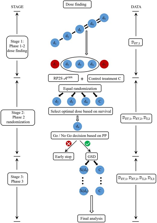
Schematic for the Gen 1-2-3 design.
Stage 1. Use a phase 1-2 design based on (YE, YT) and the criterion function |$\phi (d, \boldsymbol {\theta })$| to do sequentially adaptive dose-finding, subject to the dose acceptability rules (1). When n1 patients have been treated and evaluated, identify a candidate dose set, |${\cal A}_{n_1}^{can} \subseteq {\bf d}$|, computed from the data |${\cal D}_{ET,1}$|, as follows. Denoting the estimated criterion function of the empirically best acceptable dose by |$\hat{\phi }_{n_1}^{max}$| = |$max\lbrace \hat{\phi }_{n_1}(d):\ d\in {\cal A}_{n_1}\rbrace$|, the candidate dose set is
For example, if ρ = .70, then any acceptable dose with estimated optimality criterion at least 70% of the maximum value is a candidate.
Stage 2. For each n = n1 + 1, |$\ldots $|, n12, denote the current candidate dose set by |${\cal A}_n^{can}$|. When n2 patients have been randomized and treated, they are followed for an additional time |$L\le t^{*}_S$|, to harvest survival time data for use in later treatment evaluation. At the end of stage 2, 1 best candidate dose is selected, and a PP is computed and used as a criterion to decide whether to proceed to stage 3 and conduct a phase 3 trial.
Stage 1 may be regarded as a screening process based on early response and toxicity to reduce the number of doses for later consideration. Stage 2 completes the dose selection process, relying on survival time obtained over longer follow up as a more reliable endpoint for choosing 1 dose to obtain success in phase 3.
Selection of a best candidate dose. Under the mixture model (2), the survival function |$\overline{F}_{\rm S}(t^{*}_S \mid X(d),\boldsymbol {\theta })$| evaluated at follow up time |$t^{*}_S$| is used to select an optimal dose from |${\cal A}_{n_{12}}^{can}$|. Given the data at the end of stage 2, the optimal dose|$\hat{d}^{opt}$| is defined as the dose in |${\cal A}_{n_{12}}^{can}$| with the largest posterior probability of maximizing |$\overline{F}_{\rm S}(t_S^{*} \mid X(d),\boldsymbol {\theta })$|. Formally,
If desired, |$\hat{d}^{opt}$| may be selected using other criteria, such as the posterior mean of |$\overline{F}_{\rm S}(t_S^{*} \mid d,\boldsymbol {\theta })$|.
Go/No Go decision based on a PP. After selecting dopt, the Go/No Go decision of whether proceed to stage 3 (ie, phase 3) is made based on the PP of the hazard ratio (HR) of X(d) to C, denoted by λ(d). Denote the future phase 3 data that would become available at the end of phase 3, if it were conducted, by |${\cal D}_{S,3}^{future}$|. A parameter |$\underline{\lambda } \in (0, 1)$| must be specified to determine whether the HR of |$X(\hat{d}^{opt})$| versus C is small enough to infer that |$X(\hat{d}^{opt})$| provides a meaningful improvement in survival. At the end of stage 2, a Bayesian criterion that quantifies how |$X(\hat{d}^{opt})$| will be compared to C at the end of phase 3 is
Expression (4) is the posterior probability, given all future randomized data available at the end of phase 3, that the HR of |$X(\hat{d}^{opt})$| versus C is smaller than |$\underline{\lambda }$|. In practice, the HR cutoff |$\underline{\lambda }$| might be chosen from the range .50 to .90. Define the phase 3 success indicator |$\Xi ({\cal D}_{S,3}^{future})$| = 1 if |$\xi ({\cal D}_{S,3}^{future}) \gt p_U$| and 0 otherwise, where pU may be chosen from the range .50 to .99. If |$\Xi ({\cal D}_{S,3}^{future})$| = 1, this says that, based on all randomized data from stage 2 and a future phase 3 trial, it is likely that the HR of |$X(\hat{d}^{opt})$| compared to C is desirably small.
Since the future data |${\cal D}_{S,3}^{future}$| are not available at the end of stage 2, the Go/No Go decision is based on the predictive distribution of |${\cal D}_{S,3}^{future}$|, given the observed stage 2 randomized data,
This PP may be computed in the following steps. First, simulate a large sample of parameters |$\lbrace \boldsymbol {\theta }^{(1)},\ldots ,\boldsymbol {\theta }^{(B)}\rbrace$| from the posterior |$p(\boldsymbol {\theta }\mid {\cal D}_{ET,2}, {\cal D}_{S,2})$|. For each |$\boldsymbol {\theta }^{(b)}$|, simulate a future phase 3 dataset, |${\cal D}_{S,3}^{future, (b)}$| using the mixture model (2). Evaluate the phase 3 success indicator |$\Xi ({\cal D}_{S,3}^{future, (b)})$| using a proportional hazard model |$f_{S,PH}(y_S \mid \tau , \lambda (\hat{d}^{opt}))$| for τ = |$X(\hat{d}^{opt})$| or C. In our simulations, we assumed an independent exponential-gamma model for YS and τ = |$X(\hat{d}^{opt})$| or C to compute the posterior of |$\lambda (\hat{d}^{opt})$|. Computationally, this approach is highly efficient. Previous research (Thall et al., 2005; Zhou et al., 2020), and our simulations described below, showed that this is remarkably robust for facilitating Go/No Go decision. Nevertheless, other, more sophisticated models, such as the piecewise exponential model (Cai et al., 2014), can be used, if desired.
Repeating this computation for b = 1, |$\ldots $|, B, the estimated PP of phase 3 success is
The Go/No Go decision is to conduct phase 3 in stage 3 if |$\widehat{PP} \gt p_U(Go),$| and otherwise do not conduct phase 3 and conclude that |$X(\hat{d}^{opt})$| is not promising compared to C.
Stage 3. Using the GS design, conduct phase 3 to test the difference between the survival distributions of |$X(\hat{d}^{opt})$| and C. Each patient is followed for up to |$t^{*}_S$| months to harvest the |$(Y_S^o, \delta , \tau )$| data, for τ = |$X(\hat{d}^{opt})$| or C. The design also continues to monitor the toxicity rate |$\pi _T(\hat{d}^{opt})$| of |$X(\hat{d}^{opt})$| in stage 3 by applying the dose safety criterion given in (1) at each GS decision time, using all current toxicity data accumulated from stages 1, 2, and 3. If |$X(\hat{d}^{opt})$| is found to be excessively toxic compared to the fixed limit |$\overline{\pi }_T$|, the study is stopped and it is concluded that no X(d) is superior to C.
For the Gen 1-2-3 design, false positive decisions are more complex than those in conventional designs, and must be defined carefully. Type 1 error and family wise error rate (FWER) of the testing procedure are defined as follows to account for both survival time and toxicity, as well as dose selection. For each dose d, a generalized null hypothesis |$H_0^{gen}(d)$| may be defined to say that X(d) is not superior to C in that X(d) and C have the same survival distributions, or X(d) is unacceptably toxic compared to |$\overline{\pi }_T,$| or both. A generalized alternative hypothesis |$H_1^{gen}(d)$| then may be defined to say that X(d) is superior to C in that it has superior survival time compared to C and acceptable toxicity compared to |$\overline{\pi }_T.$| A generalized global null hypothesis then may be defined as the generalized null hypothesis being true for all doses, |$\cap _d H_0^{gen}(d)$|. The FWER is the probability of rejecting the global null in phase 3, in favor of |$H_1^{gen}(d)$| for any d, when the global null is true.
Because the Gen 1-2-3 design includes dose selection at the end of stage 2, if the Go/No Go rule says to continue to phase 3, the generalized null hypothesis |$H_0^{gen}(\hat{d}^{opt})$| being tested in phase 3 is random since |${\hat{d}}^{opt}$| is a statistic. This is the case for any design that selects the best among 2 or more experimental treatments and then compares it to a control. See, for example, the phase 2-3 designs of Thall et al. (1988) and Stallard and Todd (2003). Because phase 3 of the Gen 1-2-3 design includes both GS testing of X(dopt) versus C for survival, and safety monitoring of X(dopt) for toxicity, the generalized power of the entire procedure may be defined for a dose d* for which X(d*) provides a specified improvement in survival over C and X(d*) is safe, say with |$\pi _T^{true}(d^{*})$| = |$\overline{\pi }_T$|. For this d*, the generalized power is the probability that d* is selected, the Go/No Go rule says to Go to phase 3, and |$H_0^{gen}(d^{*})$| is rejected in favor of |$H_1^{gen}(d^{*})$| in phase 3.
3 ILLUSTRATION OF THE GEN 1-2-3 Design
3.1 Dose-outcome models
In this section, we illustrate how a Gen 1-2-3 design may be constructed by describing a particular case. We assume binary YT and YE and denote πa, b(d) = Pr(YE = a, YT = b∣d) for a, b ∈ {0, 1} and dose d, recalling that d = d0 represents C. Rather than formulating a dose-response model, for each d, we define the phase 1-2 parameter vector as the probabilities of the elementary events, |$\boldsymbol {\theta }_{ET}(d)$| = (π0,0(d), π0,1(d), π1,0(d)), with π1,1(d) = 1 − {π0,0(d) + π0,1(d) + π1,0(d)}. This model does not borrow strength between doses, but is very tractable, and is robust because it does not make any parametric assumptions about dose-toxicity or dose-efficacy curves. Given sample size n and dose d, denote the elementary event counts
for a, b ∈ {0, 1}, and denote the vector of counts by |$\boldsymbol {V}_n(d)$|. For each d, denoting n(d) = |$\sum _{i=1}^n I(\tau _i=d)$|, |$\boldsymbol {V}_n(d) \sim$| multinomial(|$n(d),\boldsymbol {\theta }_{ET}(d)$|). We denote the concatenated vectors as |$\boldsymbol {V}_n$| = |$(\boldsymbol {V}_n(0),\boldsymbol {V}_n(1),\ldots ,\boldsymbol {V}_n(J))$| and |$\boldsymbol {\theta }_{ET}$| = |$(\boldsymbol {\theta }_{ET}(0),\boldsymbol {\theta }_{ET}(1),\ldots ,\boldsymbol {\theta }_{ET}(J)).$|
We assume that the failure time is Weibull with conditional hazard function
setting β3,0 = 0 for C, so |$\boldsymbol {\theta }_{S}=(\gamma ,\psi ,\beta _1,\beta _2,\beta _{3,1},\ldots ,\beta _{3,J})$|. For sample size n ≤ n12 in stages 1 and 2, denote the early outcome data by |${\cal D}_{ET}^n=\big \lbrace (Y_{{\rm E},i}, Y_{{\rm T},i}, d_{[i]}); i=1, \ldots , n \big \rbrace ,$| and denote the randomized time-to-event data from stage 2 by |${\cal D}_{{\rm S},2}=\big \lbrace (Y^o_{{\rm S},i}, \delta _{i}, d_{[i]}); i=n_1+1, \ldots , n_{12} \big \rbrace .$| Denoting the Weibull PDF by fS and survivor function by |$\overline{F}_{\rm S}$|, the likelihood for the data at the end of stage 2 is
To complete the Bayesian model, we assume the noninformative priors
with γ and ψ ∼ γ(0.01, 0.01), and β1, β2, β3,1, |$\ldots $|, β3,J ∼ iid N(0, 102). We use MCMC to compute the posterior for |$\boldsymbol {\theta }$| given the data |${\cal D}_{12}$| = |${\cal D}_{ET}^{n_{12}} \cup {\cal D}_{{\rm S},2}$|.
The marginal survivor function at the end of follow-up is the probability weighted average
3.2 A utility-based Gen 1-2-3 design
Under this dose-outcome model, the following steps may be used to conduct a utility-based Gen-1-2-3 design. Dose-finding in stage 1 is done using the BOIN12 design (Lin et al., 2020), which relies on a numerical utility score for each of the 4 possible outcomes of (YE, YT). To establish a utility, we first assign the score U1,0 = 100 to the most desirable outcome (Y E = 1, YT = 0), and U0,1 = 0 to the least desirable outcome (Y E = 0, YT = 1). Using these 2 utilities as boundaries, we then ask the clinicians to provide their subjective utility scores U1,1 for (Y E = 1, YT = 1), and U0,0 for (YE = 0, Y T = 0). Table 1 provides an illustrative example. The mean utility of dose d based on (YE, YT), normed to take values between 0 and 1, is
which is used as a phase 1-2 dose optimality criterion, |$\phi (d,\boldsymbol {\theta }_{ET})$|. The utility-based approach has several advantages (Zhou et al., 2019; Lin et al., 2020). It is scalable and readily accommodates ordinal YE and YT, as well as more than 2 phase 1-2 endpoints (Liu et al., 2018). In addition, it contains the marginal-probabilities-based risk-benefit tradeoff method as a special case. Lastly, because Ua,b links directly to the clinical outcomes, it can easily be understood by clinicians.
Example of a utility function for 2 binary outcomes.
| YT = 0 | Y T = 1 | |
|---|---|---|
| YE = 0 | u0,0 = 40 | u0,1 = 0 |
| Y E = 1 | u1,0 = 100 | u1,1 = 60 |
| YT = 0 | Y T = 1 | |
|---|---|---|
| YE = 0 | u0,0 = 40 | u0,1 = 0 |
| Y E = 1 | u1,0 = 100 | u1,1 = 60 |
Example of a utility function for 2 binary outcomes.
| YT = 0 | Y T = 1 | |
|---|---|---|
| YE = 0 | u0,0 = 40 | u0,1 = 0 |
| Y E = 1 | u1,0 = 100 | u1,1 = 60 |
| YT = 0 | Y T = 1 | |
|---|---|---|
| YE = 0 | u0,0 = 40 | u0,1 = 0 |
| Y E = 1 | u1,0 = 100 | u1,1 = 60 |
The BOIN12 design treats |$\overline{U}(d, \boldsymbol {\theta }_{TE})$| as a “probability” and uses the quasi-binomial method to estimate its posterior, assuming a noninformative β(0.5, 0.5) prior. The posterior of |$\overline{U}(d, \boldsymbol {\theta }_{ET})$| is used to make dose escalation and de-escalation decisions, with patients adaptively allocated to the dose that optimizes the posterior mean of |$\phi (d,\boldsymbol {\theta }_{ET})$| = |$\overline{U}(d, \boldsymbol {\theta }_{TE})$|. The dose-finding algorithm of the BOIN12 design is given by Lin et al. (2020). A Gen 1-2-3 trial incorporating this utility-based phase 1-2 component may be conducted as follows:
Stage 1. Enroll the first cohort of patients at a prespecified starting dose. For each subsequent cohort, use the BOIN12 design to choose doses for up to n1 patients.
Stage 2. For sample sizes n = n1 + 1, |$\ldots $|, n1 + n2 = n12, if |${\cal A}_n^{can}$| is empty, terminate the trial. Otherwise, randomize each cohort of patients fairly among C and the doses in |${\cal A}_n^{can}$|. When desirable, |${\cal A}_n^{can}$| may be updated after each cohort. At the end of stage 2, continue to follow patients for an additional L months to collect survival time data |$(Y_S^o, \delta )$|. Select the optimal dose |$\widehat{d}^{\rm opt}$| based on an estimate of the survival probability |$\overline{F}_{\rm S}(t^{*}_S \mid X(d),\boldsymbol {\theta })$|, and make the Go/No Go decision based on the PP. Details for calculating the PP are provided in the online supporting materials. If the decision is No Go, the trial is stopped with the conclusion that X(dopt) is not promising compared to C. To ensure unbiased estimates, we estimate |$\overline{F}_{\rm S}(t^{*}_S \mid X(d),\boldsymbol {\theta })$| based only on stage 2 randomized patients. In some applications, when appropriate, stage 1 patient YS data can be leveraged for more efficient estimation using dynamic borrowing methods, such as self-adapting mixture prior (Yang et al., 2023).
Stage 3. If the Go decision is made, then a GS phase 3 trial is conducted to compare the survival time distributions of |$X(\widehat{d}^{\rm opt})$| and C. In addition, the toxicity profile of |$X(\widehat{d}^{\rm opt})$| is monitored in stage 3 at each interim analysis and at the final test to ensure that the selected dose is safe. For each interim decision, k = 1, |$\ldots $|, K − 1, after n3,k patients have been enrolled and followed for survival, 2-sided tests for superiority or futility are done using a logrank test based on the combined data |${\cal D}_{S,2} \cup {\cal D}_{S,3}.$| Denoting the approximately normal test statistic computed from the logrank statistic by Z, given futility bound |$\underline{b}_k$| and superiority bound |$\bar{b}_k$|, the trial is stopped for futility if |$|Z|\lt \underline{b}_k$|, for superiority if |$|Z|\gt \bar{b}_k$|, or for toxicity if |$\Pr \lbrace \pi _T(d,\boldsymbol {\theta }_{ET}) \lt \overline{\pi }_T \mid {\cal D}_{ET}^n\rbrace \le .10$|. Otherwise, a final test is done when a total of n3 patients have been enrolled and followed for survival in stage 3.
Due to the dose selection at the end of stage 2, a standard hypothesis testing method based on the combined data |${\cal D}_{S,2} \cup {\cal D}_{S,3}$| may have an inflated FWER. There are several ways to address this issue. One approach involves using a combination test (Bauer and Köhne, 1994), which combines the P-value based on |${\cal D}_{S,2}$| [after applying the closing test procedure (Markus et al., 1976)] with the P-value based on |${\cal D}_{S,3}$|. This approach effectively controls the FWER, but may be conservative in some cases. Another approach is to calibrate the value of pU(Go) such that the FWER inflation due to combining |${\cal D}_{S,2} \cup {\cal D}_{S,3}$| is offset by the FWER inflation caused by the early stopping at the end of stage 2. As a result, standard GS boundaries, such as the O’Brien-Fleming boundary (O’Brien and Fleming, 1979), can be used. We employ this approach in our design because it yields higher power than the combination test approach due to leveraging the FWER inflation caused by stage 2 early stopping.
The maximum sample size n3 in stage 3 depends on the accumulated numbers of patients treated with |$X(\hat{d}^{opt})$| and C, because we fix the maximum sample size for the GS design to be nGSD rather than fixing n3. For example, suppose that a GS design is planned in stage 3 with an interim analysis in the middle of the trial using a maximum sample size of nGSD = 500, and 30 patients have been treated, with 15 at each of |$X(\widehat{d}^{\rm opt})$| and C in stage 2. In stage 3, 250 − 30 = 220 patients are enrolled before the interim analysis and then, if stage 3 is continued, the additional 250 patients are enrolled after the interim analysis, which gives n3 = 220 + 250 = 470.
4 SIMULATION STUDIES
4.1 Simulation settings
In this section, we describe simulations conducted to evaluate the operating characteristics (OCs) of the utility-based Gen 1-2-3 design. Let |$\pi _T^{true}(d_j)$| denote the true toxicity probability, |$\pi _E^{true}(d_j)$| the true short-term response probability, and |$\overline{F}^{true}(t^{*}_S, d_j)$| the true survival probability at follow up time |$t^{*}_S$|. The design’s performance was evaluated under 8 scenarios having a variety of different patterns for |$\pi _T^{true}(d_j)$|, |$\pi _E^{true}(d_j)$| and |$\overline{F}^{true}(t^{*}_S, d_j)$|, shown in Figure 2.
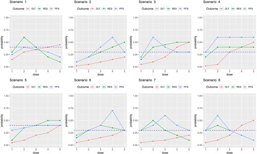
Dose-outcome curves for the scenarios in the simulation study. The dashed line represents the control.
As comparators, we used 2 conventional utility-based phase 1-2 designs followed by a phase 3 design, referred to as Conv 1 and Conv 2. The Conv 1 design consists of stages 1 and 2 of the Gen 1-2-3 design, but does not use any YS data to make decisions in these stages. Rather, an optimal dose |$\widehat{d}_{ET}^{opt}$| is selected by maximizing the posterior mean of |$\overline{U}(d, \boldsymbol {\theta }_{ET})$|. For the Conv 1 design, phase 3 is conducted to compare |$X(\widehat{d}_{ET}^{opt})$| to C if
This is a Go/No Go rule based on the ET data but no survival time data, and the decision criterion is a posterior probability rather than a PP involving simulated future data. If phase 3 is conducted, the same GS design used by Gen 1-2-3 is used in the phase 3 portion of the Conv 1 design. The Conv 2 design is similar to the Conv 1 design, with the 2 key differences that (1) C is excluded from phase 1-2; and (2) there is no Go/No Go decision between phase 1-2 and phase 3, so Conv 2 always conducts phase 3. We also considered a modified version of the CT design as a comparator. For phase 1-2, the CT design used the EffTox design, which relies on a parametric regression model with dose-response and dose-toxicity curves to borrow strength between doses, and an efficacy-toxicity tradeoff contour as a criterion for dose selection (Thall and Cook, 2004). To obtain a more fair comparison, we modified the CT design by using the same BOIN12 design and mean utility objective function in stages 1 and 2 of the Gen 1-2-3 design in the application. We refer to this as the CT-B12 design.
For the admissibility criteria (1), we set |$\overline{\pi }_T=0.35$| and |$\underline{\pi }_E=0.20$|. The fixed follow-up window for |$Y^o_S$| was |$t^{*}_S=6$| months. We also set the additional follow-up time to harvest survival time data from all patients in stage 2 who have been randomized and treated, prior to selection of optimal dose, to L = 1 month. Patients were treated in cohorts of size 3 in stage 1 and size 5 in stage 2, assuming a mean accrual rate of 1 cohort per month in stages 1 and 2 and 10 patients per month in stage 3. The maximum sample sizes were n1 = 30, n2 = 50, and nGSD = 500 for the phase 3 GS design. The remaining design parameters were ρ = 0.5, |$\underline{\lambda }=0.85$|, pU = 0.8, and pU(Go) = 0.5, determined from preliminary simulations.
As data generation models for the simulation studies, to obtain (YE, YT), we first simulated latent variables W = (WE, WT) following a bivariate normal distribution with mean (0,0), variances 1, and correlation 10. We then defined
with the cut-offs κE(dj) and κT(dj) chosen to obtain the marginal probabilities |$\pi _E^{true}(d_j)$| and |$\pi _T^{true}(d_j)$| for each dj specified under each scenario. To generate survival times, we assumed that |$t^{*}_S$| = 6, and that [YS∣YE, YT, d] followed a piecewise exponential (PE) distribution with survival
where the log hazard function takes the piecewise form
setting |$\tilde{\gamma }_{01}=\tilde{\gamma }_{0,2} = 0$| and d = d0 for C. Since |$t^{*}_S$| = 6, the parameters κE(dj), κT(dj), |$\tilde{\beta }_{01}$|, |$\tilde{\beta }_{02}$|, |$\tilde{\beta }_{E1}$|, |$\tilde{\beta }_{E2}$|, |$\tilde{\beta }_{T1}$|, |$\tilde{\beta }_{T2}$|, and |$\tilde{\gamma }_{j1},\tilde{\gamma }_{j2}$| were derived under each scenario to match the predetermined values of |$\pi _T^{true}(d_j)$|, |$\pi _E^{true}(d_j)$| and |$\overline{F}^{true}(t^{*}_S, d_j)$| for j = 0, |$\ldots $|, 5. For theoretical consistency, if desired, the final interval for defining the PE hazard may be extended to be infinite to ensure that the distribution of all possible YS is well defined.
4.2 Simulation results
Table 2 summarizes OCs of the Gen 1-2-3, Conv 1, Conv 2, and CT-B12 designs, including optimal dose selection percentages at the end of stage 2, final comparative treatment decision percentages at the end of stage 3, mean number of patients treated with each dose of X and with C, mean trial duration by month, mean overall sample size, mean percentage of Go decisions, and the mean percentage of Go decisions with the true optimal dose, given that a Go decision is made (in parentheses). All results are based on 5000 simulated replicates of the trial using each design.
Dose selection %, Final Trt % = percent of times the final conclusion is that X(d) is better than C, mean number of patients treated with each dose (0* for the control), mean trial duration in months, mean sample size, and percent Go decisions.
| Dose levels | ||||||||||
|---|---|---|---|---|---|---|---|---|---|---|
| Design | 0* | 1 | 2 | 3 | 4 | 5 | Dur trial | Sample size | % Go | |
| Scenario 1 | ||||||||||
| |$\pi _T^{true}(d_j)$| | .20 | .15 | .30 | .35 | .40 | .45 | ||||
| |$\pi _E^{true}(d_j)$| | .30 | .30 | .60 | .40 | .20 | .10 | ||||
| |$\overline{U}^{true}(d_j)$| | 50.0 | 52.0 | 64.0 | 50.0 | 36.0 | 28.0 | ||||
| |$\overline{F}^{true}(t^{*}_S, d_j)$| | .40 | .25 | .40 | .35 | .30 | .20 | ||||
| Gen 1-2-3 | Dose Sel % | 1.2 | 26.1 | 50.9 | 18.9 | 2.9 | 0 | 33.7 | 198.7 | 32.5 |
| Final Trt % | 94.7 | 2.8 | 1.1 | 1.1 | 0.3 | 0 | ||||
| # Pats | 75.6 | 30.7 | 62.1 | 25.1 | 4.5 | 0.8 | ||||
| Conv 1 | Dose Sel % | 1.4 | 17.8 | 70.2 | 10.4 | 0.2 | 0.0 | 43.3 | 283.8 | 52.3 |
| Final Trt % | 94.8 | 2.5 | 1.3 | 1.4 | 0.0 | 0.0 | ||||
| # Pats | 117.5 | 26.5 | 114.9 | 21.6 | 2.5 | 0.8 | ||||
| Conv 2 | Dose Sel % | 1.4 | 16.9 | 73.0 | 8.5 | 0.2 | 0.0 | 65.7 | 479.4 | 100 |
| Final Trt % | 77.4 | 16.3 | 3.8 | 2.3 | 0.2 | 0.0 | ||||
| # Pats | 200.1 | 64.1 | 180.4 | 30.9 | 3.0 | 0.8 | ||||
| CT-B12 | Dose Sel % | 1.6 | 43.1 | 24.6 | 22.3 | 6.7 | 1.7 | 62.5 | 447.2 | 100 |
| Final Trt % | 45.2 | 41.8 | 1.4 | 5.0 | 4.9 | 1.7 | ||||
| # Pats | 200.1 | 99.0 | 75.3 | 52.8 | 16.7 | 3.3 | ||||
| Scenario 2 | ||||||||||
| |$\pi _T^{true}(d_j)$| | .10 | .02 | .05 | .10 | .15 | .20 | ||||
| |$\pi _E^{true}(d_j)$| | .30 | .10 | .20 | .30 | .40 | .50 | ||||
| |$\overline{U}^{true}(d_j)$| | 54.0 | 45.2 | 50.0 | 54.0 | 58.0 | 62.0 | ||||
| |$\overline{F}^{true}(t^{*}_S, d_j)$| | .30 | .10 | .20 | .40 | .60 | .30 | ||||
| Gen 1-2-3 | Dose Sel % | 0.1 | 0.9 | 5.5 | 20.4 | 64.0 | 9.1 | 48.1 | 312.6 | 80.9 |
| Final Trt % | 29.2 | 0.3 | 2.0 | 11.7 | 56.4 | 0.4 | (69.7) | |||
| # Pats | 126.1 | 11.7 | 18.2 | 48.1 | 81.8 | 26.7 | ||||
| Conv 1 | Dose Sel % | 0.1 | 2.0 | 6.1 | 16.8 | 32.4 | 42.6 | 34.9 | 207.2 | 36.3 |
| Final Trt % | 83.0 | 0.2 | 0.3 | 3.4 | 12.2 | 0.9 | (33.6) | |||
| # Pats | 73.3 | 11.7 | 14.5 | 25.3 | 31.8 | 50.7 | ||||
| Conv 2 | Dose Sel % | 0.0 | 1.4 | 5.1 | 15.1 | 30.9 | 47.5 | 61.5 | 435.3 | 100 |
| Final Trt % | 51.2 | 1.4 | 4.4 | 10.1 | 30.9 | 2.0 | ||||
| # Pats | 177.6 | 14.6 | 26.6 | 51.1 | 57.2 | 108.1 | ||||
| CT-B12 | Dose Sel % | 0.0 | 22.9 | 21.8 | 21.9 | 21.2 | 12.2 | 58.9 | 409.2 | 100 |
| Final Trt % | 23.3 | 22.9 | 16.6 | 14.9 | 21.2 | 1.1 | ||||
| # Pats | 177.5 | 34.1 | 55.9 | 58.3 | 42.3 | 41.1 | ||||
| Scenario 3 | ||||||||||
| |$\pi _T^{true}(d_j)$| | .10 | .05 | .10 | .20 | .40 | .50 | ||||
| |$\pi _E^{true}(d_j)$| | .30 | .15 | .40 | .45 | .50 | .50 | ||||
| |$\overline{U}^{true}(d_j)$| | 54.0 | 47.0 | 60.0 | 59.0 | 54.0 | 50.0 | ||||
| |$\overline{F}^{true}(t^{*}_S, d_j)$| | .30 | .20 | .60 | .40 | .30 | .30 | ||||
| Gen 1-2-3 | Dose Sel % | 0.1 | 2.5 | 73.2 | 18.4 | 4.8 | 1.0 | 46.6 | 297.5 | 81.7 |
| Final Trt % | 26.3 | 0.7 | 63.1 | 9.9 | 0.0 | 0.0 | (77.2) | |||
| # Pats | 120.7 | 15.8 | 93.9 | 47.9 | 15.8 | 3.5 | ||||
| Conv 1 | Dose Sel % | 0.1 | 1.6 | 27.8 | 39.3 | 26.1 | 5.1 | 40.1 | 253.4 | 45.3 |
| Final Trt % | 77.2 | 0.3 | 9.2 | 12.0 | 1.1 | 0.2 | (20.3) | |||
| # Pats | 98.1 | 14.5 | 32.4 | 58.6 | 39.7 | 10.2 | ||||
| Conv 2 | Dose Sel % | 0.1 | 1.0 | 32.5 | 38.7 | 24.4 | 3.3 | 62.7 | 446.7 | 100 |
| Final Trt % | 37.4 | 0.7 | 32.5 | 27.8 | 1.3 | 0.3 | ||||
| # Pats | 183.4 | 18.2 | 67.8 | 109.5 | 58.4 | 9.4 | ||||
| CT-B12 | Dose Sel % | 0.2 | 27.8 | 31.4 | 19.7 | 16.5 | 4.4 | 60.5 | 425.2 | 100 |
| Final Trt % | 33.1 | 22.2 | 31.4 | 12.3 | 0.7 | 0.3 | ||||
| # Pats | 186.8 | 67.9 | 58.8 | 60.2 | 40.9 | 10.7 | ||||
| Scenario 4 | ||||||||||
| |$\pi _T^{true}(d_j)$| | .10 | .02 | .05 | .30 | .40 | .50 | ||||
| |$\pi _E^{true}(d_j)$| | .30 | .20 | .40 | .40 | .40 | .40 | ||||
| |$\overline{U}^{true}(d_j)$| | 54.0 | 51.2 | 62.0 | 52.0 | 48.0 | 44.0 | ||||
| |$\overline{F}^{true}(t^{*}_S, d_j)$| | .30 | .30 | .60 | .60 | .60 | .60 | ||||
| Gen 1-2-3 | Dose Sel % | 0.0 | 4.1 | 50.5 | 32.3 | 10.5 | 2.6 | 47.0 | 294.3 | 92.2 |
| Final Trt % | 17.0 | 0.4 | 46.8 | 29.8 | 5.9 | 0.1 | (83.1) | |||
| # Pats | 119.7 | 23.5 | 77.8 | 50.2 | 18.2 | 5.0 | ||||
| Conv 1 | Dose Sel % | 0.0 | 4.1 | 48.0 | 33.2 | 11.8 | 2.9 | 30.4 | 164.0 | 33.1 |
| Final Trt % | 67.2 | 0.0 | 14.2 | 12.5 | 5.0 | 1.1 | (80.7) | |||
| # Pats | 54.3 | 17.0 | 43.3 | 32.0 | 13.8 | 3.7 | ||||
| Conv 2 | Dose Sel % | 0.0 | 3.2 | 50.2 | 32.0 | 11.4 | 3.2 | 51.6 | 336.3 | 100 |
| Final Trt % | 2.9 | 0.3 | 50.2 | 32.0 | 11.4 | 3.2 | ||||
| # Pats | 128.1 | 25.4 | 93.8 | 59.1 | 22.8 | 7.0 | ||||
| CT-B12 | Dose Sel % | 0.0 | 27.2 | 22.3 | 31.3 | 14.2 | 5.0 | 52.6 | 345.8 | 100 |
| Final Trt % | 26.3 | 0.9 | 22.3 | 31.3 | 14.2 | 5.0 | ||||
| # Pats | 147.4 | 63.3 | 54.7 | 49.9 | 22.8 | 7.9 | ||||
The percent of Go decisions at the truly optimal dose is given in parentheses. Boldface indicates values for the true optimal final decision.
Scenario 1 is a null case where no dose d gives X(d) with better survival than C. Because a Go/No Go decision is included in the Gen 1-2-3 and the Conv 1 designs, both may stop the trial early, at the end of stage 2. The Gen 1-2-3 design correctly concludes that no X(d) is superior to C 94.7% of the time, with a similar value 94.8% for the Conv 1 design. This percentage drops to 77.4% for the Conv 2 design and 45.2% for the CT-B12 design. For each design, the FWER as a percentage is 100 minus this value, specifically |$5.3\%$| for Gen 1-2-3, |$5.2\%$| for Conv 1, |$22.6\%$| for Conv 2, and |$54.8\%$| for CT-B12. Gen 1-2-3 and Conv 1 have much shorter trial durations of 33.7 and 43.3 months, and much smaller sample sizes of 198.7 and 283.8, compared to the respective durations 65.7 and 62.5 months and sample sizes 479.4 and 447.2 for the Conv 2 and CT-B12 designs. In addition, the Gen 1-2-3 design has a 32.5% chance of conducting phase 3. These results quantify the substantial advantages obtained by including a Go/No Go decision rule.
In scenario 2, d4 is truly optimal with the highest |$\overline{F}^{true}(t^{*}_S, X(d_4))$| = 0.60, whereas d5 has the highest mean utility |$\overline{U}^{true}(X(d_5))$| = 62 but is suboptimal with |$\overline{F}^{true}(t^{*}_S, X(d_5))$| = 0.30. The Gen 1-2-3 design has the highest percentage, 56.4%, of correctly concluding that X(d4) is superior to C, an 80.9% chance of making a Go decision, and 69.7% of the Go decisions result in the conclusion that X(d4) is superior. In contrast, the correct final conclusion percentages for X(d4) are 12.2%, 30.9%, and 21.2% under the Conv 1, Conv 2, and CT-B12 designs. For patient allocation, the Gen 1-2-3 design assigns an average of 81.8 patients to d4, compared to 31.8, 57.2, and 42.3 for the Conv 1, Conv 2, and CT-B12 designs. The Conv 1 and Conv 2 designs assign most patients, 50.7 and 108.1, to d5, which has the highest mean utility. The CT-B12 design assigns patients evenly among the doses, with the numbers ranging from 34.1 to 58.3. For trial duration and mean sample size, the designs with a Go/No Go decision, Gen 1-2-3 and Conv 1, have better results than Conv 2 and CT-B12. In scenario 3, d2 is truly superior to C, with |$\overline{F}^{true}(t^{*}_S, X(d_2))$| = 0.60 compared to |$\overline{F}^{true}(t^{*}_S, X(d_0))$| = 0.30, and d2 also has the highest mean utility. The Gen 1-2-3 design again outperforms all other designs, with at least a 30% higher correct final decision percentage, and it also assigns at least 26 more patients to d2.
In scenario 4, doses d2, d3, d4, and d5 all have the same survival probability .60 at 6 months, but d2 and d3 have acceptable toxicity rates of .05 and .30, while d4 and d5 have unacceptably high toxicity rates of .40 and .50. Thus, there are 2 true optimal treatments, X(d2) and X(d3), in this scenario. However, X(d2) is preferable due to its much smaller toxicity probability .05, compared with .30 for X(d3). The Gen 1-2-3 design performs well compared to the Conv 1 and CT-B12 designs, with a |$76.6\%$| chance of concluding that X(d2) or X(d3) is superior to C. Between the 2 truly superior doses, the Gen 1-2-3 design slightly favors X(d2), with a higher correct final conclusion percentage of |$46.8\%$| and a larger number of patients, 77.8. This is because the Gen 1-2-3 design uses the posterior mean utility for dose screening and randomization in stage 2, and the utility function accounts for toxicity. The Conv 2 design has a slightly better performance than the Gen 1-2-3 design in this scenario. This is because the Conv 2 design selects the optimal dose based on the mean utility, and doses d2 and d3, both of which are truly superior to C in terms of survival, have larger mean utility values than the other doses in scenario 4. Additionally, there is no Go/ No Go decision in the Conv 2 design, which further increases the generalized power of the design. However, as seen in scenario 1, the Conv 2 design fails to control the FWER if there is no truly superior dose. Additional simulation results, for scenarios 5, 6, 7, and 8, are given in Table S1 of the online supplementary materials. The results are qualitatively similar to those obtained for scenarios 1, 2, 3, and 4.
4.3 Sensitivity analyses
We performed additional simulations to explore the sensitivity of the Gen 1-2-3 design to several of is parameters. The results are summarized in the online supporting information. The simulations in Table 2 were based on pU(Go) = 0.5 for the Go/No Go decision. Table S2 summarizes the OCs of the Gen 1-2-3 design using each of the values pU(Go) = 0, 0.5, and 0.9, where pU(Go) = 0 implies that phase 3 always is conducted. As expected, larger pU(Go) is more favorable under the null scenarios 1 and 5, while smaller pU(Go) is more favorable when a truly optimal experimental treatment X(dj) exists for j = 1, |$\cdots $|, or 5, in scenarios 2-4 and 6-8. Considering both null and alternative scenarios, it appears that pU(Go) = 0.5 is the best cutoff to obtain generally good performance. A possible reason that pU(Go) = 0.5 works well is that the Go/No Go decision serves as a screening rule, and when making a screening decision, it may be more desirable to use a relatively low cut-off value that primarily eliminates very unpromising doses. If a dose d for which X(d) in fact does not improve survival compared to C passes the Go/No Go decision, the chance that the subsequent GS test will conclude X(d) is superior to C still is low.
Table S3 shows the effects of using different randomization methods in stage 2. We denote equal randomization in Table 1 by ER, and consider 2 alternative methods. Method 2, referred to as Half, randomizes half of the patients to C and uses AR for the doses in |${\cal A}_{n}^{can}$|. Method 3 uses AR to randomize patients among C and the doses in |${\cal A}_n^{can}$|. The results show that ER and AR give very similar overall performances, and both outperform Half. It thus appears that stage 2 of the Gen 1-2-3 design does not require the use of AR.
Table S4 studies the effect of different additional follow-up times L on the OCs of the Gen 1-2-3 designs. The results confirm that larger L improves the Go/No Go decision, and therefore can generally give better performances for final treatment comparisons to C and patient allocation. The changes in mean sample size are minimal, but the total trial duration is prolonged. In practice, L should be chosen, based on preliminary simulations, in terms of the tradeoff among correct treatment selection, patient allocation, and trial duration.
Table S5 considers different types of candidate dose sets. In Table S5, an alternative |${\cal A}_{n_1}^{can}$| was defined that uses only the n1 patients in stage 1 and keeps this set unchanged thereafter. The results show that these 2 ways to define a candidate dose set yield similar performances. In particular, |${\cal A}_{n}^{can}$| performs slightly better than |${\cal A}_{n_1}^{can}$| under the null scenarios and |${\cal A}_{n_1}^{can}$| is slightly better than |${\cal A}_{n}^{can}$| under the alternative scenarios. Also, using |${\cal A}_{n_1}^{can}$| increases the mean sample size slightly.
Table S6 evaluates robustness of the Gen 1-2-3 design to different parametric models to generate the survival outcomes for the simulation studies. In addition to the piecewise exponential model used in Table 1, the Weibull and log-logistic distributions for survival time also are considered in this table. The results show that different distributions for survival time give very similar OCs, which confirms the robustness of the exponential-gamma model.
To further evaluate the FWER using the Gen 1-2-3 design beyond the null scenarios 1 and 5, Table S7 considers additional scenarios in which no X(d) is superior to C in terms of survival and also safe in terms of toxicity. Scenarios S1 and S2 are cases where all doses are safe but none of them has better survival than C. In scenarios S3 and S4, doses d4 and d5 are overly toxic, and there is either no dose with better survival than C (scenario S3), or the dose with superior survival is unsafe (scenario S4). In scenarios S5 and S6, all doses are overly toxic. Figure S1 depicts the empirical FWER of the Gen 1-2-3 design under these scenarios. The results show that the Gen 1-2-3 does a good job of controlling overall FWER around a nominal level of 5% across this set of scenarios.
5 DISCUSSION
Stages 1 and 2 of a Gen 1-2-3 design may be thought of as a refined dose screening and selection process based on both early and late outcomes. Stage 1 uses efficacy and toxicity with conventional phase 1-2 design machinery to assign patients sequentially to doses, screen out unsafe or ineffective doses, and reduce the original dose set to the candidates |${\cal A}_{n_1}^{can}$|. This step in stage 1 is important because identifying a candidate dose set rather than selecting 1 optimal dose allows the dose space to be explored more fully based on survival time in subsequent stages. Stage 2, which may be regarded as a link between sequentially adaptive phase 1-2 dose finding and phase 3, has 4 key elements. (1) Including C ensures that each X(dj) evaluation is based on a comparison to C, and (2) randomization ensures that these comparisons are unbiased. (3) In contrast with conventional phase 1-2 designs, the dose optimization criterion is based on survival time, YS, rather than on the early (YE, YT) outcomes. Finally, (4) stage 2 includes a Go/No Do decision based on a PP that X(dopt) is superior to C in terms of survival. This greatly reduces the risk of wasting resources conducting a phase 3 trial of an agent that is unlikely to provide a meaningful survival benefit over C, and thus it helps to control the FWER.
Rather than fixing the maximum sample size for the phase 3 GS design to be nGSD, an alternative approach that might be preferred by a drug developer would determine the phase 3 sample size n3 adaptively based on the phase 1-2 survival data available at the end of stage 2 along the line of sample size recalculation. This would require an additional computation, possibly based on a sensitivity analysis of the design for a range of n3 values, using predictive probabilities, and also require further calibration of decision boundaries to ensure FWER control.
While we have constructed the phase 3 GS decision rules to compare survival using frequentist logrank tests, if desired, Bayesian posterior criteria could be used instead as test statistics. For example, the k th posterior decision criterion for comparing survival in stage 3 might be Pr|$\lbrace \overline{F}_{\rm S}(t_S^{*} \mid \hat{d}^{opt},\boldsymbol {\theta }) \gt \overline{F}_{\rm S}(t_S^{*} \mid {d_0},\boldsymbol {\theta }) \mid data_k \rbrace$||$\gt \overline{b}_k$| for superiority, and |$\lt \underline{b}_k$| for futility, or possibly median survival time for |$\hat{d}^{opt}$| and d0 could be used. While this would make the design’s decision rules more fully Bayesian, it still would be necessary to calibrate all design parameters to obtain good OCs.
For trial conduct, given that an institution has the resources to conduct phase 1-2 and phase 3 trials, the main additional practical requirement of a Gen 1-2-3 design is the inclusion of stage 2 between a phase 1-2 design and phase 3, including computations for the decisions, dose screening, and randomization implemented by the computer program. Due to its additional structure and complexity, the necessary computer simulations required to construct a Gen 1-2-3 design may be time-consuming, and certainly will require careful planning and interactions between statisticians and physician investigators. Our simulations indicate that this additional effort is warranted, since they show that the Gen 1-2-3 design has very desirable properties compared to more conventional approaches.
Acknowledgement
The authors thank the Associate Editor and two referees for valuable comments.
FUNDING
Y.Z.’s research was partially supported by the National Institutes of Health (NIH) grants R01 GM150808, R21 CA264257, P30 CA082709, and the Ralph W. and Grace M. Showalter Research Trust award. P.T.’s research was supported by the NIH/National Cancer Institute (NCI) grants 1R01CA261978, 5P30 CA016672, and 5P01CA148600. Y.Y.’s research was supported by the NIH/NCI grants P50 CA098258, P50 CA217685, and P50 CA221707.
CONFLICT OF INTEREST
None declared.
DATA AVAILABILITY
Data sharing is not applicable to this article as no new data were created or analyzed in this paper.
