


ABSTRACT
Motivated by the problem of accurately predicting gap times between successive blood donations, we present here a general class of Bayesian nonparametric models for clustering. These models allow for the prediction of new recurrences, accommodating covariate information that describes the personal characteristics of the sample individuals. We introduce a prior for the random partition of the sample individuals, which encourages two individuals to be co-clustered if they have similar covariate values. Our prior generalizes product partition models with covariates (PPMx) models in the literature, which are defined in terms of cohesion and similarity functions. We assume cohesion functions that yield mixtures of PPMx models, while our similarity functions represent the denseness of a cluster. We show that including covariate information in the prior specification improves the posterior predictive performance and helps interpret the estimated clusters in terms of covariates in the blood donation application.
1 INTRODUCTION
Human blood is an essential resource in global health care, for example, in acute emergencies, surgical interventions, or for the survival of chronic patients. To understand its relevance, before COVID-19, the demand was about 10 million units per year in the United States and 2.1 million in Italy (World Health Organization, 2012), and these values are constantly growing. Unfortunately, blood cannot be produced in a laboratory. It can only be withdrawn from healthy unpaid volunteers, at least in Western countries, and its short shelf life limits the period between withdrawal and use.
In modern healthcare systems, blood is supplied by the Blood Donation Supply Chain (BDSC), which provides adequate blood units to meet the demand of transfusion centers and hospitals (Baş et al., 2016). Blood collection is the first echelon of the BDSC, and it has a relevant impact on the entire system in terms of blood unit flow. A key issue lies in the uncertainty associated with the arrival of donors at the collection centers. Thus, predicting donations and their temporal distribution is crucial to better feed and control the entire BDSC.
This work has been motivated by applicative and methodological goals. The applicative purpose is to compute accurate predictions of donation times for the enrolled donors in a blood collection center or, equivalently, of gap times between successive blood donations as we do in this work. As a first task, the prediction of gap times supports the planning of donation activities. This is important not only for the internal organization of the center, to dimension human and material resources necessary for processing the incoming donors on each collection day, but also for the integration of collection with the other echelons of the blood supply chain. For the blood center internal organization, the prediction of gap times for all eligible donors provides the overall capacity required to serve the donors, independently of their blood type (Lanzarone and Yalçındağ, 2020). At the same time, from the production viewpoint, it supplies the production of units for each blood type in a given time horizon.
As a second task, gap time prediction influences the profiling of the donors. Blood collection centers invest, also in economic terms, to carry out campaigns to promote and acquire further donors. The goal is to enroll novel donors who regularly and frequently donate blood. Promotion campaigns should target individuals whose characteristics guarantee high donation frequency and continuity over the years, that is, those with short and stable gap times associated with higher productivity. Our approach is able to infer the clustering structure of the donors and, at the same time, the prediction of their gap times, to highlight which groups are more productive (eg, students versus workers, younger versus elder). As a result, the collection center will be able to appropriately choose the target of a promotion campaign directing it toward the most promising profiles.
There is relatively limited literature on the prediction of gap times between successive blood donations: for instance, Bosnes et al. (2005) predict the number of donors that will arrive on a given date, Fortsch and Khapalova (2016) estimate ARMA models for total daily blood demand, or James and Matthews (1996) analyze blood donor return behavior using frequentist survival analysis methods. Our data have been collected at the Milano Department of the Associazione Volontari Italiani del Sangue, referred to as AVIS in the following, which serves a large hospital in the same city (Niguarda hospital). Like many blood collection centers, AVIS requires proper planning of donation activities and, at the same time, aims at properly profiling donors. They aim to determine whether homogeneous clusters of donors can be detected, and whether those are characterized by specific patterns of recurrent donation times and similar donors’ characteristics (given by personal and registry information). The dataset includes donors who did not exit the recurrent donation process in the time window we consider (6.5 years). Therefore, we address them as loyal donors in the rest of the paper.
From the methodological viewpoint, we propose suitable Bayesian models for clustering donors using recurrent event data. The models allow the prediction of new recurrences, accommodating for covariate information that describes the personal characteristics of the sample individuals. At the same time, we use covariate information of the individuals in the prior distribution of the random partition of the sample individuals themselves. The Bayesian framework naturally handles model-based clustering assuming that the random parameter of the model includes the partition of the sample subjects (Hartigan, 1990; Quintana and Iglesias, 2003). We introduce a prior encouraging two subjects to co-cluster a priori if their corresponding covariate values are similar.
Covariate-dependent priors in a Bayesian nonparametric context are relatively new. The seminal work in this area is MacEachern (1999). However, reference papers with clustering with covariates are Müller and Quintana (2010) and Müller et al. (2011). In these works, the prior on the random partition is given via cluster-specific cohesion and similarity functions. The cohesion function |$c$| typically depends only on the cluster size, while the similarity |$g$| is a non-negative function that formalizes the similarity among the covariates in the cluster. The covariate-dependent prior is given through a product partition approach as
where |$\rho _n$| denotes the partition of the |$n$| sample subjects and |$\mathbf {x}_j^{*}= \lbrace \mathbf {x}_i, i \in A_j\rbrace$| denotes the collection of covariates corresponding to items belonging to the |$j$|th cluster |$A_j$|, being |$\mathbf {x}_i$| the vector of covariates of individual |$i$|. In Müller and Quintana (2010) and Müller et al. (2011), the cohesion function is derived from the Dirichlet process and the similarity |$g$| is the marginal distribution of covariates |$\mathbf {x}_j^{*}$| in an auxiliary probability model, even if the |$\mathbf {x}_i$|, |$i =1, \dots , n$|, are not assumed random. The prior introduced product partition models with covariates (PPMx). For similar approaches, possibly including variable selection or spatial dependence, see Park and Dunson (2010), Quintana et al. (2015), Barcella et al. (2016), Page and Quintana (2016), Page and Quintana (2018), and Page et al. (2022). Alternative models with dependent priors for random partitions are in Dahl et al. (2017), Dahl (2008), Blei and Frazier (2011), and Bianchini et al. (2020).
Our covariate-dependent prior generalizes (1) into two directions: (|$i$|) to mitigate the rich-get-richer property, we depart from the cohesion function of the Dirichlet process and assume the cohesion function |$c$| generated by a more general class of random probability measures, namely the normalized completely random measures (Regazzini et al., 2003); (|$ii$|) we consider similarity functions |$g$|, which are not marginal densities; borrowing the idea from data-driven clustering approaches, we introduce |$g$|’s measuring the denseness of covariates in each cluster. In this paper, we use denseness to denote a measure of proximity of the covariate vectors in a cluster, that is, a cluster is dense when the total distance between covariates in the cluster and the associated centroid is small. The resulting model turns out to be a mixture of PPMx models as in (1), allowing the construction of a general Markov chain Monte Carlo (MCMC) sampler, which does not depend on the specific choice of similarity.
We first describe the model for a unidimensional regression setting. Then, we consider a more general model for AVIS data using a longitudinal approach for the sequence of the logarithms of gap times (the responses) between recurrent events that are blood donations. In the latter case, since the observed log-gap times are skewed, we assume a skew-normal distribution for the response (Azzalini, 2005; Arellano-Valle and Azzalini, 2006). We propose three different similarity functions, discussing how their analytical properties might influence posterior inference, and we apply two of them in the simulated examples and the motivating application. Since the analytic normalizing constants of some of the full-conditionals of our MCMC are unknown, we cannot assume that the hyperparameters of the cohesion or of the similarity functions are random. However, we later discuss how to set these hyperparameters. The design of an MCMC sampler for the computation of posterior inference is among the contributions of our paper, also accommodating for the longitudinal nature of the responses and the skew-normal sampling model for the blood donation application. We extend the augmented marginal Gibbs sampler for normalized completely random measures mixture models by Favaro and Teh (2013).
We mention here that our prior |$\pi (\rho _n \mid \mathbf {x}_1, \dots , \mathbf {x}_n)$|, as well as the PPMx prior and its generalizations (1), has the attractive property of encouraging individuals with equal or similar covariates to be co-clustered. Nevertheless, this type of priors does not have the marginal invariance property, that is, the prior of the random partition for |$n$| individual cannot be obtained as the marginal of the prior of the random partition for |$n+1$| individuals.
2 BAYESIAN COVARIATE DRIVEN CLUSTERING
In a regression context, let |$y_i\in {\mathbb {R}}$| be the observed value of the response random variable |$Y_i$|, and let |$\mathbf {x}_i\in {\mathbb {R}}^m$| be the covariate vector of the |$i$|th observation. We denote by |$\mathbf {y}_j^{*}$| (or |$\mathbf {x}_j^{*}$|) the set of all responses |$y_i$| (or covariates |$\mathbf {x}_i$|) in cluster |$A_j$|, with |$\mathbf {y}^{*}_j = \lbrace y_i, i \in A_j \rbrace$| (equivalently |$\mathbf {x}^{*}_j = \lbrace \mathbf {x}_i, i \in A_j \rbrace$|). We assume that responses are independent across groups, conditionally on covariates and the cluster-specific parameters, distributed according to a regression sampling model. The regression parameters are cluster-specific and are assumed i.i.d. from a base distribution |$P_0$|. The prior on the partition depends on covariates through a similarity function. We then assume
where |$f(\mathbf {y}_j^{*}\mid \mathbf {x}^{*}_j, \mathbf {\theta }_j^{*})=\prod _{i\in A_j}^{}f(y_i;\mathbf {x}_i,\theta ^{*}_j)$|, |$n_j$| is the size of cluster |$A_j$|, |$g(\mathbf {x}_j^{*})$| is the similarity function on cluster |$A_j$|, and |$P_0$| is a non-atomic probability measure on |$\Theta$|. The likelihood specification in (2) may be any model, from simple regression models as in Web Appendix C, to the more complex models for gap times of recurrent events as the case study of Section 4. The functions |$D$| and |$c$| in (4) are defined as
and |$\zeta (s)$|, |$s\gt 0$|, is a positive function, denoted as Lévy intensity. Note that, when |$g\equiv 1$|, (4) and (5) define a prior that can be equivalently introduced as the prior induced on a sample of |$n$| latent variables from a normalized completely random measure (Regazzini et al., 2003), which encompasses the Dirichlet process under a suitable choice of |$\zeta$|. One of the major advantages of normalized completely random measures is that prior (4) with |$g\equiv 1$| is particularly robust for cluster estimation, implying heavy tails of the associated prior of the number of clusters |$k_n$| and strongly mitigating the rich-get-richer property of the Dirichlet process. See Lijoi et al. (2007) and Argiento et al. (2015) for further details on mixtures driven by normalized completely random probability measures.
Equation 4 is the integral with respect to |$u$| of some integrand function, and, because defining the prior of our model parameter |$\rho _n$|, it enters into the full-conditionals of the Gibbs sampler for posterior inference. Being an integral, it is generally difficult to be numerically evaluated. However, note that the integrand function is a PPMx for each fixed |$u$|, with cohesion |$c(\cdot ,u)$| and similarity function |$g$|. Hence, if we prove that |$U=u$| can be interpreted as an auxiliary random variable, that is, if we can compute its marginal distribution, (4) can be explained as a mixture of PPMx. Consequently, using a standard augmentation approach, the integral in (4) is disintegrated by adding |$u$| to the state space of the associated MCMC. When |$g\equiv 1$|, this disintegration approach has been successfully used; see Favaro and Teh (2013) and Argiento and De Iorio (2022).
To show that |$\pi (\rho _n \mid \mathbf {x}_1, \dots , \mathbf {x}_n)$| in (4) is well defined, we remark that, by assuming that |$g$| takes values in (0,1], we have
The last equality follows from Pitman (2003), Corollary 6. Consequently, the marginal density of the mixing variable |$U$| is
All these comments justify the name PPMx-mixt for the prior (4). Note that covariates that enter the similarity function do not need to be necessarily the same as those in the regression part of the likelihood. Still, they can be selected specifically for each application.
For concreteness, the presentation focuses on a cohesion function arising from a specific normalized completely random measure, the normalized generalized gamma process, denoted by |$\mathrm{NGG}(\kappa , \sigma , P_0)$|. Such a choice recovers as particular cases several models commonly used in the Bayesian nonparametric literature, such as the Dirichlet process (Ferguson, 1973), the normalized inverse-Gaussian process (Lijoi et al., 2005), and the normalized |$\sigma$|-stable process (Pitman, 2003). The Lévy intensity of the NGG process is given by |${\displaystyle \zeta (ds) = \frac{\kappa }{\Gamma (1-\sigma )} s^{-1-\sigma }\mathrm{e}^{-s}\mathbb {1}_{(0,+\infty )}(s) ds}$|, where |$\sigma \in [0,1)$| is a discount parameter and |$\kappa \gt 0$| is the total mass parameter. In this case, the cohesion function equals
Parameter |$\sigma$| has a strong impact on the clustering structure. In particular, when |$g\equiv 1$|, the larger is |$\sigma$|, the more dispersed the number of clusters is. This feature mitigates the annoying the rich-get-richer effect, typical of the Dirichlet process, leading to more size-balanced clusters. For more details on the behavior of |$\sigma$| in NGGs, see for instance Lijoi et al. (2007) and Argiento et al. (2010, 2015). The Gibbs sampler Pólya urn scheme for model (2)-(4) is detailed in Web Appendix C.
The lack of marginal invariance of the prior for the random partition prevents us to compute posterior predictive distributions for new individuals as the integral of the sampling model with respect to the posterior distribution. However, we deal with this calculation considering the responses of new individuals as missing data and including the associated new covariates in the set of all covariates values. For an alternative approach, based on an importance sampling re-weighting step, see Müller et al. (2011).
3 THE CHOICE OF THE SIMILARITY FUNCTION
In this paper, a cluster is dense when the sum of the distances between each covariate in the cluster and the associated centroid is small. We consider similarity functions |$g$|, with |$0\lt g\le 1$| (see Section 2), which quantifies the denseness of the cluster through covariates. To this end, let us denote |$g(\mathbf {x}^{*}_j):= g(\mathcal {D}_{A_j})$|, where
|$d$| is some distance between vectors and |$\mathbf {c}_{A_j}$| is the centroid of the set of covariates in cluster |$j$|, here assumed as the Fréchet mean. We assume that |$g$| is a decreasing (ie, non-increasing) function of |$\mathcal {D}_{A_j}$|, so that the smaller is |$\mathcal {D}_{A_j}$| (and hence the denser is the cluster |$A_j$|), the larger is the value |$g(\mathbf {x}^{*}_j)$|. We let |${\mathbf {x}}_i=({\mathbf {x}}^c_i, {\mathbf {x}}^b_i)$|, where |${\mathbf {x}}^c_i$| (of size |$m_c$|) and |${\mathbf {x}}^b_i$| (of size |$m_b$|) are the available continuous and binary covariates, respectively. We define the function |$d(\cdot , \cdot )$| in (7) as
where |$d_c$| and |$d_b$| denote the Mahalanobis and the normalized Hamming distances.
We propose a list of similarity functions based on preliminary studies in Bianchini (2018): (|$i$|) |${\displaystyle g_A(\mathbf {x}^{*}_j; \lambda ) = \mathrm{e}^{-t^\alpha }}$|, for |$\alpha \gt 0$|; (|$ii$|) |${\displaystyle g_B(\mathbf {x}^{*}_j; \lambda ) = \mathrm{e}^{-\alpha \log (1 + t)}}$|, for |$\alpha \gt 0$|; (|$iii$|) |$g_C(\mathbf {x}^{*}_j; \lambda )=\mathrm{e}^{-t \log (1 + t)}$|. Here, |$t = \lambda \mathcal {D}_{A_j}$|.
Hyperparameter |$\lambda$| is responsible for rescaling the range of values of |$\mathcal {D}_{A_j}$|, where we evaluate the similarity function. It is the analog to the temperature parameter defined in Dahl et al. (2017) and it tempers how covariates impact the prior. The power parameter |$\alpha$| drives the influence of the covariates in the prior of the random partition, by stretching or compressing the function over its support. Typical values for |$\alpha$| are |$1/2,1,2$|. Figure 1 shows the graphs of the three similarities as a function of |$t\ge 0$|. Similarity functions |$g_A$| and |$g_B$| are intuitive, that is, their behavior for |$t\rightarrow +\infty$| is exponential and polynomial, respectively. As far as |$g_C$| is concerned, we have proposed the expression |$\mathrm{e}^{-t\log (1 + t)}$| in such a way that, for large |$t$|, we contrast the asymptotic behavior of the Gamma function in the cohesion (6) induced by the NGG. Note that, |$\mathcal {D}_{A_j\cup \lbrace i\rbrace }\ge \mathcal {D}_{A_j}$|, where |$\lbrace i \rbrace$| is a singleton; see Web Appendix A (S1). This implies that the function |$g$| penalizes large clusters that are not dense at the same time. This is exactly the feature we would like to guarantee to mitigate the rich-get-richer property of the cohesion function associated with the Dirichlet process.

Left: plot of the similarity functions for |$\alpha =1$| and |$\lambda =1$|; right: plot of |$g_C$| for different values of |$\lambda$|.
We propose a heuristic strategy to fix |$\lambda$|: given the available data, we estimate the increment of |$\mathcal {D}_{A_j}$| when we add the new observation |$\lbrace \mathbf {x}_i\rbrace$| across all possible values of the sample size of |$A_j$|. For instance, for any sample size |$n_j$| from 2 to |$n$|, we uniformly choose a cluster |$A_j$| of size |$n_j$|, and we add a point |$i$| (not in |$A_j$|), to obtain a Monte Carlo estimate of the increment |$(\mathcal {D}_{A_j \cup \lbrace i\rbrace } - \mathcal {D}_{A_j})$|. We average over the sample size |$n_j$|, obtaining an estimate |$\hat{\varepsilon }$|. Then, we choose |$\lambda$| such that |$\lambda \hat{\varepsilon }= \varepsilon ^{*}$|, for small values of |$\varepsilon ^{*}$|, that is, |$\varepsilon ^{*}= 10^{-1}, 10^{-2}, 5 \times 10^{-3}$|. The choice of |$\varepsilon ^{*}$|, and consequently of |$\lambda$|, calibrates the influence of the similarity function in the posterior estimated clusters, which might be over-driven by covariate values. For a thorough discussion about the calibration of similarities in PPMx models, see Page and Quintana (2018).
The specification of a PPMx-mixt prior consists in choosing a cohesion function, |$c(u;n_j)\ge 0$| for |$n_j \in \lbrace 1, \ldots , n\rbrace$|, and a non-negative similarity function |$g$|. The former quantifies the probability mass of a generic cluster |$A_j$|, |$j = 1,\dots ,k_n$|, through its cardinality, conditioning to |$u\gt 0$| and regardless of the knowledge of the subjects in |$A_j$|, while the latter formalizes the similarity of the covariates. The similarity function affects posterior inference through the posterior predictive law reported in (S5) and (S6) of Web Appendix C. The first formula shows that there are two factors, the first depending only on the responses |$y_i$|’s through the marginal density of data in cluster |$j$|, while the second factor depends on the cohesion and the similarity, that is,
The ratio between cohesions |$c(u,n_j+1)$| and |$c(u,n_j)$| assume values proportional to |$n_j-\sigma$|, and consists in the usual predictive weight in NGG mixture models. Henceforth, we focus on the ratio between the similarity values. For |$\lambda$| fixed as we have described above, let |$t=\lambda \mathcal {D}_{A_j}$| and |$t+\varepsilon = \lambda \mathcal {D}_{A_j \cup \lbrace i\rbrace }$|, so that |$\varepsilon$| represents the increment of the average center-based distance when |$\lbrace \mathbf {x}_i\rbrace$| is assigned to cluster |$A_j$|. So, it is interesting to study |$g(t+\varepsilon )/g(t)$|, for |$t\gt 0$| and any fixed |$\varepsilon \gt 0$|. This ratio is smaller or equal than 1, since |$g$| is non-increasing. It is advantageous to have a ratio that assumes small values when |$t$| is large to discourage non-dense clusters. The function |$g_C$| is the only one to fulfill this requirement, among the three similarities proposed here, as shown in Figure 1 in Web Appendix B. The same figure shows that the ratio is constant for |$g_A$|, and it is increasing for |$g_B$|. Similarly, it is interesting to study the ratio |$g(t+\varepsilon )/g(t)$| also as a function of |$\varepsilon \gt 0$|, for any fixed value of |$t \gt 0$| which, of course, is non-increasing with |$\varepsilon$|. Hence, when we add observation |$i$| in cluster |$A_j$|, two scenarios can occur: (1) the new observation is similar to the others belonging to |$A_j$|, so |$\varepsilon$| is small, and the ratio is close to one, yielding to a weak penalization of the weight of the cluster |$A_j \cup \lbrace i\rbrace$|; (2) the new observation strongly differs from the elements in |$A_j$|, so |$\varepsilon$| is large and the ratio becomes small. In this case, the model strongly penalizes the weight of the cluster |$A_j \cup \lbrace i\rbrace$|.
A simulation study to compare the effect of the similarity functions |$g_A$| and |$g_C$| on posterior distribution is shown in Web Appendix E. A comparison with alternative models using benchmark data is given in Web Appendix F.
4 BLOOD DONATION DATA APPLICATION
Our data concern new donors of whole blood, donating between January 1st, 2010 and May 15th, 2016 in the main building of AVIS Milano. By a new donor, we mean a blood donor who has donated for the first time after January 1st, 2010. Data are recurrent donation times, with extra information summarized in a set of covariates, collected by AVIS physicians. Donors include only loyal individuals, that is, a new donation is expected within a finite amount of time with probability one. The resulting dataset contains |$11\, 505$| donations, made by |$2\, 912$| donors; the number of gap times between recurrent donations varies from 1 to 20.
The statistical focus is the clustering of donors according to the trajectories of gap times and the computation of accurate prediction of donation times. Figure 2 reports the histogram of gap times (in the |$\log$|-scale) for men and women.
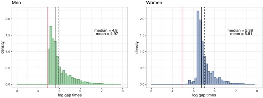
Histogram of the logarithm of the observed gap times grouped by gender; male donors on the left and female donors on the right. The red line denotes the minimum waiting time between two donations, according to the Italian law. The black continuous and dashed lines denote the empirical median and mean, respectively.
The skewness of these histograms can be explained since, according to the Italian law, the maximum number of whole blood donations is 4 per year for men and 2 for women, with a minimum of 90 days between one donation and the next. In the dataset, the minimum for men is around 4.47 (|$\mathrm{e}^{4.47} \simeq 87$| days), while the median gap time for men is 121 days. For women, the distribution has a median of approximately 5.24 in the log scale: this means 189 days, corresponding to about 6 months. Donors may donate before the minimum imposed by law, under good donor’s health conditions and the physician’s consent. Figure S2 in Web Appendix B reports the mean and median trajectories of gap times for any recurrence |$j=1,\ldots , 20$|. Donors enter the study randomly in the whole time window. The number of donors for each |$j=1,\ldots ,20$| is decreasing: there are |$2\, 912$| donors with at least the first gap time, but only two with 20 gap times.
Among different covariates available, we selected some of them, which are known to be associated with the gap times, according to a preliminary study (see Gianoli, 2016): Gender (indicator of gender, 1 if woman, 0 if man); Blood group (4-level categorical variable, equal to 0, A, B, and AB); RH (rhesus factor, 1 if it is positive, 0 if negative); Smoke (indicator of smoking habit, ie, 1 if the donor regularly smokes, 0 otherwise); Age (age in years at the first donation at the entrance in the study); BMI [body mass index (at the entrance in the study)]. Covariates such as weight, height, and smoke are not directly controlled by AVIS physicians, but are communicated by donors themselves so that they can be inaccurate. See the last line of Table 3 for the empirical frequencies of the categorical covariates listed above. Sample statistics of the age (in years) at the first donation give that the minimum is 18, the maximum is a maximum of 68, empirical quantiles of order 25%, 50%, 75% equal to 27, 35, 44, while the empirical mean and standard deviation are 33.83 and 10.27. Analogous sample statistics for the BMI values at first donation are 21.56, 23.93, and 25.70 (sample quartiles) and 23.93 and 3.37 (sample mean and standard deviation).
4.1 A framework for recurrent events
Let |$n$| be the number of individuals (donors) and |$T_{i,t}$| be the time of the |$t$|th donation of donor |$i$|. We assume that |$0:=T_{i,0}$| corresponds to the time of first donation for each |$i$| and that individual |$i$| is observed over the time interval |$[0,\tau _i]$|, where |$\tau _i$| denotes the censoring time of the |$i$|th observation. If |$m_i$| events are observed at times |$0\lt T_{i,1}\lt \cdots \lt T_{i, m_i} \lt \tau _i$|, let |$W_{i,t}=T_{i,t}-T_{i,t-1}$| for |$t=1,\ldots ,m_i$| denote the waiting times (gap times) between events of subject |$i$| and |$W_{i,m_i+1}= T_{i,m_i+1}-T_{i,m_i}$|, assuming that |$T_{i,m_i + 1} \gt \tau _i$| denotes the |$(m_i + 1)$|th gap time for the |$i$|th donor censored at time |$\tau _i$|. We assume that the study has been administratively censored, that is, censoring and observations are independent. Further, our approach considers the time of all first donations as known. We aim to model the waiting times |$W_{i,t}, t = 1, \dots , m_i$|, for |$i = 1, \dots , n$|, by incorporating some exogenous information in the prior distribution of the latent partition in the form of covariates.
Let |$Y_{i,t} = \log (W_{i,t})$| for all |$i$| and all |$t$|, and let |${\boldsymbol Y}_i:=(Y_{i,1}, \dots , Y_{i,m_i},Y_{i,m_i+1})$|. We assume that gap times are conditionally independent within clusters, that is, |$f(\mathbf {y}^{*}_j\mid \mathbf {x}^{*}_{j}, \theta _j^{*}) = \prod _{i\in A_j}f({\boldsymbol y}_i|\mathbf {x}_{i}, \theta _j^{*})$|, but differently from Section 2, each |${\boldsymbol Y}_i$| has dimension |$m_i+1$|. Furthermore, the evaluation of the sampling distribution includes the information on the censoring of the |$(m_i+1)$|th gap time for each |$i=1,\ldots ,n$|. It is clear from Figure 2 that the assumption of gaussianity for observed data |$Y_{i,t} = \log (W_{i,t})$|’s is not appropriate, while the more flexible assumption of skew-normality would fit the dataset. For each |$t=1,\ldots , m_i+1$| and each |$i$| in cluster |$A_j$|, |$j = 1, \dots , k_n$|, we assume that
where |$\eta _{i,t}$| are latent variables from the standard half-normal distribution and |$s_i$| represents the cluster allocation of individual |$i$|. Note that (9) corresponds to assuming that |$Y_{i,t}$| has a skew-normal distribution. Skew-normal mixture models have been employed in the Bayesian framework, as, for instance, Bayes and Branco (2007), Frühwirth-Schnatter and Pyne (2010), Arellano-Valle et al. (2007), and Canale et al. (2016). For a definition and its properties, see Azzalini (2005) and Arellano-Valle and Azzalini (2006). In (9), the conditional distributions of the gap times on the log scale in cluster |$A_j$| share the group-specific parameter |$\theta _j^{*}=(\alpha _j,\psi _j,\sigma ^2_j)$|. We omit the asterisk on the right to avoid heavier notation. Following Frühwirth-Schnatter and Pyne (2010), |$\alpha _j$| is the random intercept, |$\psi _j/\sigma _j$| is the skewness parameter, and |$\sigma _j$| is a scale parameter. From (9), the expectation of |$Y_{i,t}$|, in addition to the two linear terms, is |$\alpha _j+\psi _j\sqrt{2/\pi }$|, while its variance is |$\sigma _j^2+\psi _j^2(1-2/\pi )$|.
As far as the linear predictor is concerned, we distinguish regression parameters corresponding to fixed-time covariates (|${\boldsymbol \beta }_0$|) from the parameters referring to time-varying covariates (|${\boldsymbol \beta }_t$|), and |${\mathbf {x}}_{i}$| includes |$p_1$| fixed-time covariates and |${\mathbf {x}}_{it}$| denotes |$p_2$| time-varying covariates. No intercept is included in the linear predictor to avoid identification issues with the cluster-specific random intercept |$\alpha _j$|. The prior we assume is described as follows:
The number |$k_n$| of cluster-specific parameters is determined by |$\rho _n$|, and is random. Notation |$\mathrm{IG}(\cdot ;a,b)$| denotes the inverse-gamma density with mean |$b/(a-1)$| and |$\mathrm{diag}(\xi ^2_1,\dots , \xi ^2_{p_2} )$| is a diagonal matrix, which entries |$\xi ^2_1,\dots , \xi ^2_{p_2}$|. In our specific case, |$p_2 = 1$| and the distributions of |$\boldsymbol{\beta }_1, \dots , \boldsymbol{\beta }_J$| collapse on a univariate Gaussian distribution, where |$J=\max _{i}(n_i+1)$| is the maximum number of gap times. Notation PPMx-mixt denotes the prior described in Section 2. We assume that the cohesion function |$c(u, n_j)$| and the Lévy intensity |$\zeta (\mathrm{d}s)$| correspond to the NGG process. The choice of |$P_0$| yields conjugacy of the associated full-conditional (see Frühwirth-Schnatter and Pyne, 2010).
The same covariates may enter into the linear predictor and the prior of the random partition. In this application, after preliminary covariate choice via LPML (log pseudo marginal likelihood, Christensen et al., 2010) evaluation, we choose to include Gender, Blood group, RH, Smoke, and BMI (at the first donation) in the linear term, so that |$p_1=7$| considering dummy variables too. The only time-varying covariate included in the linear term is Age at the |$t$|th donation. Only static covariates enter the prior of the random partition: Gender, Blood Group, RH, Smoke, Age at the first donation and BMI at the first donation.
4.2 Posterior inference
To perform posterior inference for model (9)-(13), we modify the Gibbs sampler in Web Appendix C to consider the likelihood of recurrent events. See Web Appendix D for details. We fix hyperparameters as follows: |$\Sigma _0=\mathrm{diag}(1,\dots ,1)$|, |$(\nu _0, \tau _0) = (2, 1)$|, |$\alpha _0 = \psi _0=0$| and |$\kappa =0.5$| [see (6)]. Since |$n_j-\sigma$| is the unnormalized weight that a new item is assigned to cluster |$A_j$|, |$\sigma$| in (6) is a key hyperparameter; we assume three different values for |$\sigma$| and report the associated posterior estimates in Table 1 for sensitivity analysis. The distance |$d(\mathbf {x}_i, \mathbf {x}_j)$| entering the similarity function’s definition is given in (8). Every run of the Gibbs sampler produced a final sample size of |$10\, 000$| iterations, after a burn-in of |$5\, 000$| iterations. Convergence was checked in all simulations using visual inspection and standard diagnostics as in Figure S3 of Web Appendix B.
Log pseudo marginal likelihood (LPML) and number of clusters in the estimated partition, obtained minimizing a posteriori VI, for the blood donation data, for different values of |$\lambda$| and |$\sigma$|, and similarities |$g_C$|, |$g\equiv 1$|.
| |$g_C$| | |$g\equiv 1$| | |$PPMx$| | |||||
|---|---|---|---|---|---|---|---|
| |$\lambda$| | |$\sigma$| | LPML | |$\hat{K}_{\mathrm{VI}}$| | LPML | |$\hat{K}_{\mathrm{VI}}$| | LPML | |$\hat{K}_{\mathrm{VI}}$| |
| 0.005 | 0.001 | −22 032.51 | 5 | −22 424.91 | 5 | −21 850.19 | 8 |
| 0.010 | 0.001 | −22 068.25 | 5 | ||||
| 0.100 | 0.001 | −21 812.24 | 6 | ||||
| 0.005 | 0.150 | −21 990.26 | 6 | −22 252.37 | 6 | ||
| 0.010 | 0.150 | −21 758.68 | 5 | ||||
| 0.100 | 0.150 | −21 221.55 | 5 | ||||
| 0.005 | 0.300 | −22 150.35 | 5 | −22 311.26 | 7 | ||
| 0.010 | 0.300 | −22 012.24 | 6 | ||||
| 0.100 | 0.300 | −21 672.05 | 7 | ||||
In evidence: the best model in terms of LPML.
Table 1 shows the number of clusters of the estimated partition and LPML values with similarity functions |$g_C$| and |$g\equiv 1$| (no covariates in the prior), for different values of the temperature hyperparameter |$\lambda$| and the reinforcement parameter |$\sigma$|. By definition, the larger the LPML is, the better the model fits the data. There is a clear effect of |$\sigma$|, |$\lambda$| and covariates (through |$g_C$|) on LPML: the best value corresponds to |$\lambda =0.1$| and |$\sigma =0.15$|. Values of LPML for |$g_C$| are much larger than in the case of |$g\equiv 1$|. For any of the hyperparameter values in the table, we have computed an estimate of the random partition for the sample donors, minimizing a posteriori the expectation of the variation of information (VI) loss function (see, for instance, Wade and Ghahramani, 2018). We report the number |$\hat{K}_{\mathrm{VI}}$| of estimated clusters in Table 1. Since the cardinality of the visited partitions is quite large, as suggested by Wade and Ghahramani (2018), from the MCMC estimate of the posterior co-clustering matrix, we consider all the partitions designed by a hierarchical clustering algorithm with complete linkage. Then, as the point estimate, we select the partition that achieves the minimum value of the posterior loss function. It is clear that |$\hat{K}_{\mathrm{VI}}$| is robust with respect to the effect of covariates in the prior and changes in |$\sigma$| and |$\lambda$|, though as expected, |$\hat{K}_{\mathrm{VI}}$| increases with |$\sigma$|. This is an aspect of the well-known trade-off between the estimation of the number of clusters and the posterior predictive checks, especially in the case of misspecified models (see, for instance Beraha et al., 2022, Section 7). Typically, the posterior predictive check improves when overestimating the number of clusters.
The rest of the posterior inference reported below is computed for the optimal values of the hyperparameters, that is, |$\lambda = 0.100$| and |$\sigma = 0.150$|. Note that |$\sigma =0.001$| in Table 1 approximates the cohesion function yielded by the Dirichlet process as in Müller and Quintana (2010) and Müller et al. (2011) (though they use a different similarity).
Table 2 shows posterior means of the regression coefficients of the fixed-time covariates. All the fixed-time covariates included in the study are significantly different from zero; see the last column. The average log-gap time increases for donors with blood groups 0, A, and B with respect to the reference level AB. Of course, women exhibit longer gap times in accordance with the Italian law. Figure S4 in Web Appendix B shows the regression coefficients for the only time-dependent covariate included in the study (age of the donor). All these parameters are significantly different from zero. Further, as the occasion of donation increases, the impact of age on the log-gap time decreases in magnitude, implying that loyal donors are less subject to age differences.
Posterior summaries of the fixed-time regression coefficients |$\boldsymbol \beta _0$| for the blood donation application.
| Covariate | Median | |$95\%$| C.I. | |$\max \lbrace \Pr (\beta _j \gt 0), \Pr (\beta _j \lt 0)\rbrace$| |
|---|---|---|---|
| BMI | −0.060 | (−0.077; −0.043) | 1.000 |
| Gender | 1.119 | (0.938; 1.329) | 1.000 |
| Blood group 0 | 1.137 | (0.779; 1.480) | 1.000 |
| Blood group A | 1.131 | (0.768; 1.486) | 1.000 |
| Blood group B | 1.230 | (0.755; 1.692) | 1.000 |
| RH | 0.533 | (0.295; 0.755) | 1.000 |
| Smoke | 0.339 | (0.148; 0.526) | 0.999 |
BMI: body mass index.
Figure 3 shows the trajectories of the observed log-gap times grouped by the estimated clusters as explained before. It is clear from the cluster sizes that the rich-get-richer property of the cohesion associated with the Dirichlet process is here mitigated. We do not observe substantial differences among the log-gap times in the estimated clusters. However, Cluster 1 seems to group longer trajectories (see also the number of donations per cluster in Table 3).
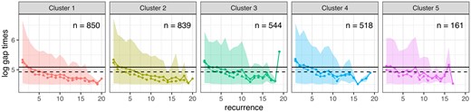
Recurrent gap times (on the log scale) by estimated cluster for the blood donation application. We draw each cluster’s sample mean (continuous line), median (dashed line), and the 90% sample quantile band. The black continuous and dashed lines denote the overall mean and median, respectively.
Empirical summaries of covariates, number of donations, and log gap-times within each estimated cluster for the blood donation application.
| Age | BMI | Gender | Blood group | RH | Smoke | No. donations | Log gap-time | |||||
|---|---|---|---|---|---|---|---|---|---|---|---|---|
| Female | A | B | AB | 0 | + | Yes | Mean (SD) | Mean (SD) | ||||
| Cl. 1 | 46.81 | 24.48 | 36.35% | 40.29% | 12.51% | 3.34% | 43.86% | 88.92% | 32.78% | M | 4.99 (4.05) | 4.92 (0.48) |
| F | 2.92 (2.19) | 5.46 (0.42) | ||||||||||
| Cl. 2 | 33.92 | 24.11 | 29.06% | 38.59% | 11.88% | 3.18% | 46.35% | 87.18% | 37.53% | M | 4.52 (3.86) | 4.98 (0.53) |
| F | 2.44 (1.73) | 5.55 (0.43) | ||||||||||
| Cl. 3 | 28.16 | 23.77 | 33.64% | 34.01% | 12.13% | 3.49% | 50.37% | 87.13% | 31.07% | M | 4.82 (3.76) | 4.99 (0.49) |
| F | 2.62 (1.75) | 5.50 (0.34) | ||||||||||
| Cl. 4 | 22.83 | 22.95 | 32.24% | 38.22% | 12.16% | 5.02% | 44.59% | 84.94% | 27.80% | M | 3.63 (3.14) | 5.03 (0.54) |
| F | 2.39 (1.69) | 5.58 (0.42) | ||||||||||
| Cl. 5 | 20.26 | 23.79 | 7.45% | 37.89% | 14.91% | 8.70% | 38.51% | 77.64% | 27.95% | M | 4.59 (3.13) | 5.00 (0.49) |
| F | 3.25 (2.34) | 5.41 (0.29) | ||||||||||
| All | 33.83 | 23.93 | 31.39% | 38.11% | 12.33% | 3.91% | 45.64% | 86.74% | 32.69% | M | 4.55 (3.76) | 4.97 (0.51) |
| F | 2.64 (1.91) | 5.51 (0.41) | ||||||||||
The cluster summaries in the last two columns are given per gender. BMI: body mass index.
Table 3 reports empirical summaries of the covariates (included in the prior) within each estimated cluster, that is, empirical means for continuous covariates and empirical frequency for the binary or categorical covariates. The last two columns display the empirical average and standard deviation for the number of recurrences (|$m_i$|’s) and the log gap times per cluster, grouped by gender. Cluster 1 groups older donors, since the cluster mean is one standard deviation above the overall mean. These donors also have a slightly higher BMI and a higher percentage of women. From Figure 3, it is also clear that those donors have longer trajectories of gap times. On the other hand, Table 3 shows that the average number of donations in Cluster 1 is higher than the overall empirical averages for men and women.
Cluster 2 contains donors with empirical averages of covariates (but for the indicator of smoking) and the number of donations close to the corresponding overall empirical means. Cluster 3 groups younger donors than Cluster 2, with fewer smokers. Clusters 4 and 5 group very young donors and Cluster 5 is mostly made of men with a high percentage of blood type |$0^-$|. However, donors in Cluster 4 donate less than average for both genders. The clusters do not show clear differences as far as the log gap times are concerned. We have also compared the cluster estimates reported above (|$\lambda =0.1$|, |$\sigma =0.15$|) for |$g_C$|, with competitor models: (|$i$|) |$g\equiv 1$| and |$\sigma =0.15$| (no effect of covariates in the prior), (|$ii$|) |$\lambda =0.1$| and |$\sigma =0.001$| for |$g_C$|, that is, cohesion function corresponding to the Dirichlet process and (|$iii$|) the original PPMx in Müller et al. (2011). See Web Appendix G. The estimated clusters under the original PPMx prior are less clearly interpretable in terms of covariates than ours.
4.3 The impact of posterior estimates on AVIS planning and profiling
Accurate prediction of gap times between successive blood donations of donors impacts donor profiling and donation planning. Currently, AVIS does not use any particular data-driven method for predicting blood supply. There is a target level provided by Niguarda hospital but AVIS aims at producing as much blood as possible regardless of this target. In the event of overproduction, the excess blood is typically transferred from Niguarda hospital to another facility. Instead, the critical problem is the production imbalance of each blood type between days, which makes it difficult to store blood in Niguarda hospital facility. Hence, a tool predicting donors’ gap times would allow the design of robust scheduling systems that properly redirect donors to the most appropriate days. This would also reduce the imbalance of blood production between days. The scheduling system currently adopted by AVIS is deterministic and does not include donor arrival predictions (Baş et al., 2018).
The estimated clustering structure is particularly useful for the profiling problem. The 5 estimated clusters correspond to diverse typologies of donors, as highlighted by the covariates associated with each cluster. Therefore, according to our analysis, donor recruitment campaigns should be directed toward the older donors identified by Cluster 1, since they can guarantee high donation frequency and continuity over the years. These campaigns could be organized, for instance, by setting up mobile healthcare facilities for blood donations near the working sites where we expect to find individuals belonging to Cluster 1 (eg, big companies with old employees).
5 DISCUSSION
In this work, we propose a regression model for gap times of recurrent events, where parameterization includes the partition |$\rho _n$| of the blood donors through cluster-specific random effects modeled as a PPMx-mixt. We assume a skew-normal conditional distribution for the logarithm of gap times between blood donations from AVIS. The prior we fix for |$\rho _n$| encompasses covariate information, encouraging two individuals to be co-clustered if they have similar covariate values. We have seen that including covariate information in a similarity function improves the posterior predictive performance and helps interpret the estimated clusters in terms of covariates. By introducing a latent variable |$u\gt 0$|, we can express the cohesion function in the prior, and hence the whole prior for the random partition of the sample, as a mixture of PPMx. We propose three examples of similarity functions, emphasizing their properties and their effects on the posterior predictive distribution of the model. Cross-validated posterior predictive root mean-squared errors (Web Appendix G) for the AVIS dataset show that the inclusion of the similarity function |$g$| in the prior for the random partition yields a lower value than in the case with no covariates in the prior. We estimate 5 clusters of homogeneous donors. This grouping also helps identify individuals’ characteristics and important features (covariates), supporting profiling for effective campaigns to acquire further donors. Comparison to cluster estimates under the original PPMx formulation (Müller et al., 2011) shows a larger number of clusters for the latter prior, which do not seem easier to explain in terms of covariates. The similarity functions |$g$| that we propose must be calibrated via a parameter |$\lambda$|, and we discuss how to fix it. This is a key parameter that prevents the overpowering effect of covariates on clusters with respect to likelihood.
An interesting characteristic of our model is that, though it clusters donor gap times trajectories, it allows us to interpret the estimated clusters also in terms of other features. In particular, our model considers covariate information: some of the estimated clusters are similar when looking at the response trajectories, but different when looking at the covariates. We believe this aspect is an advantage of all models with covariate-dependent prior for the random partition—including ours—as it allows for greater flexibility and interpretability.
We have assumed a continuous conditional distribution for the logarithm of the gap times, which are expressed in days. However, these data are grouped, according to the definition in Tutz and Schmid (2016), that is when the continuous time is divided into intervals and, if the event has occurred in the morning of the |$s$|th day, one says that it has been observed at “day |$s$|,” with |$s$| integer. Modeling continuous distributions to represent discrete data shows advantages: larger flexibility of continuous distributions, computational efficacy especially in the case of MCMC algorithms, and greater interpretability of the parameters of continuous distributions. Continuous distributions are more convenient when we represent the posterior predictive densities on the real line. On the other hand, using discrete distributions to represent the likelihood could be useful when event times are intrinsically discrete (which is not the case here), or when we model the hazards (which are conditional probabilities for discrete data).
The pitfall of our strategy consists in its computational cost. Future work may consider using approximate sampling strategies to overcome this limitation.
Acknowledgement
The authors are grateful to Dr Ilaria Bianchini for her contribution to the construction of the model and the computational strategy at an early stage of this manuscript. Her work has been part of her Ph.D. thesis. The authors also thank Dr Sergio Casartelli, general manager of AVIS Milano, for kindly providing data and support for the interpretation of the posterior inference.
FUNDING
R.A and A.G. have been partially supported by MUR - Prin 2022 - Grant no. 2022CLTYP4, funded by the European Union – Next Generation EU.
CONFLICT OF INTEREST
None declared.
DATA AVAILABILITY
The Associazione Volontari Italiani del Sangue (AVIS) dataset of Section 4 contains sensitive information and cannot be shared publicly, due to the privacy of individuals that participated in the study. In agreement with AVIS Milano, a sub-sample of anonymized data of 100 donors is available in the Supplementary Materials.
