


ABSTRACT
Precision medicine is an approach for disease treatment that defines treatment strategies based on the individual characteristics of the patients. Motivated by an open problem in cancer genomics, we develop a novel model that flexibly clusters patients with similar predictive characteristics and similar treatment responses; this approach identifies, via predictive inference, which one among a set of treatments is better suited for a new patient. The proposed method is fully model based, avoiding uncertainty underestimation attained when treatment assignment is performed by adopting heuristic clustering procedures, and belongs to the class of product partition models with covariates, here extended to include the cohesion induced by the normalized generalized gamma process. The method performs particularly well in scenarios characterized by considerable heterogeneity of the predictive covariates in simulation studies. A cancer genomics case study illustrates the potential benefits in terms of treatment response yielded by the proposed approach. Finally, being model based, the approach allows estimating clusters’ specific response probabilities and then identifying patients more likely to benefit from personalized treatment.
1 INTRODUCTION
Cancer comprises a collection of complex diseases characterized by heterogeneous cellular alterations across patients and cancer cells within the same neoplasm (Bedard et al., 2013). Patients with similar clinical diagnoses may show diverse responses to the same treatment due to tumor heterogeneity. A treatment for a particular diagnosis may be effective on average, but its effectiveness may vary across subpopulations. In recent years, many attempts have been made to devise personalized treatment strategies that leverage patients’ characteristics, including the tumor’s genome, to identify the treatment with the highest likelihood of success (Simon, 2010). Within this precision medicine paradigm, there is an increasing interest in discovering individualized treatment rules (ITRs) for patients who show heterogeneous responses to treatment, for example, when the treatment effect varies across groups of patients. An ITR is a decision rule that assigns the patient to the treatment given patient/disease characteristics (Ma et al., 2015). The optimal ITR is the one that maximizes the population mean outcome. Statistical methodology research in precision medicine is devoted to developing personalized treatment rules to inform decision-making. The distinctive mark of statistical inference under the precision medicine paradigm is to leverage heterogeneity to improve therapeutic strategies (Kosorok and Laber, 2019).
Our interest specifically lies in developing frontline treatment selection rules rather than estimating treatment’s causal effects, as commonly done within the ITR framework. Conventional methods for treatment selection rules are based on semi- and nonparametric procedures to identify subgroups of patients more likely to benefit from a treatment leveraging few baseline markers (Bonetti and Gelber, 2000; Song and Pepe, 2004). The subgroup approach can provide valuable information when performed according to a prespecified analysis plan. Nonetheless, stratified subsets of patients defined by one or few biomarkers are often inadequate to account for patient heterogeneity and ultimately fail to establish effective treatment selection rules (Pocock et al., 2002). Other approaches account for patient heterogeneity by including covariates (Zhang et al., 2012; Zhao et al., 2012). However, for these methods, the correct definition of treatment-by-marker interactions is crucial and relies on sensitive assumptions, which are difficult to specify in the clinical practice and may be limited to generalized linear models (Ma et al., 2016).
To overcome these limitations, Ma et al. (2016, 2018, 2019) have established a hybrid 2-step predictive model for personalized treatment selection. In the first step, a clustering algorithm based on a predefined genomic signature (predictive markers) is used to obtain a heuristic measure of the patients’ molecular similarity. In the second step, given this measure of patients’ similarity and a set of prognostic markers, a Bayesian model is used for treatment selection; specifically, for a new, untreated patient, the model predicts the treatment response probabilities for each competing treatment. This framework establishes 2 significant improvements over existing methods. Firstly, the common assumption of statistical exchangeability among patients is relaxed. Since each tumor is unique, patients are considered partially exchangeable only to the extent to which their tumors are molecularly similar. Moreover, this approach utilizes complementary sources of information for treatment selection, integrating predictive and prognostic characteristics of a patient.
This paper proposes a Bayesian predictive model for personalized treatment selection that builds upon Ma et al. (2019) and overcomes some of its main limitations. As in Ma et al. (2019), we leverage prognostic determinants and predictive biomarkers for treatment selection. We propose a fully Bayesian integrative framework for clustering and prediction that performs all inferential tasks in a single model avoiding multistep procedures; the proposed approach results in a treatment selection rule that fully accounts for patients’ heterogeneity. Note that in Ma et al. (2019), the patients’ similarities were estimated in the first step and included as known quantities in the second step; moreover, in the first step, 2 arbitrary choices had to be made, namely the clustering algorithm and the number of clusters. The proposed method accounts for the uncertainty in all modeling steps, resulting in improved prediction performances. In particular, we use a product partition model with covariates (PPMx, Müller et al., 2011) to cluster observations that are similar in terms of the values of the predictive covariates; specifically, the predictive covariates enter the model through the prior for the random partition. The resulting partitions are only partially exchangeable, and patients with similar covariates are a priori more likely to be clustered together. In this paper, we use the cohesion function induced by the normalized generalized gamma process (NGGP) as a building block of our PPMx model to mitigate the rich-get-richer property of the Bayesian nonparametric (BNP) priors. Namely, the rich-get-richer is the tendency for a small number of clusters to become overrepresented as more data points are added to the process, resulting in few large clusters and potentially many singletons. Despite being well studied in the BNP literature as a prior inducing a Gibbs-type random partition (Lijoi et al., 2007), NGGP still has no common use. To the best of our knowledge, this is one of the first attempts the NGGP is employed as cohesion function in a PPMx model (see Argiento et al., 2022).
We devise a method that, given the patients’ prognostic and predictive markers, assigns them to the treatment with the highest likelihood of positive response. Prognostic covariates influence disease progression regardless of the treatments given to the patient, whereas predictive covariates change the likelihood of a positive response to a particular treatment. Conceptually, our strategy for selecting the optimal treatment for the new, untreated patient can be broken down into 3 steps. First, we consider historical patients and cluster them separately for each treatment according to their predictive markers. In this way, patients who underwent the same treatment are divided into homogeneous clusters with respect to predictive biomarkers. Then, we compute the utility provided by each competing treatment to the new untreated patient by assigning the new patient to the subgroup of historical patients with whom he shows the largest similarity in terms of predictive markers. The utility function relies on the model’s posterior predictive distribution, which depends on both prognostic and predictive biomarkers. Finally, we select the treatment that ensures the largest predicted benefit.
We apply the proposed method to a brain cancer dataset (Ma et al., 2019), comprising 158 patients equally assigned to either standard or targeted treatment. For each patient, prognostic and predictive biomarkers, both consisting of preselected genomic markers, are available in addition to their categorical response to treatment. To facilitate optimal treatment selection, we assign numerical utilities to each treatment response level. This leads to a median utility score, which serves as a 1-dimensional criterion for treatment selection. Our model shows good predictive performances and provides a sound framework for the identification and interpretation of clusters of patients.
2 BAYESIAN INTEGRATIVE MODEL
We consider n historical patients treated with T alternative treatments, whose predictive and prognostic biomarkers are measured along with a discrete set of response levels of the clinical outcome. Let a = 1|$,\ldots,$|T be index treatments and |$n = \sum _{a=1}^{T}n^a$| be the total number of treated patients, of which na assigned to therapy a. Note that, in our notation, the superscript a is solely a treatment index. The treatment response |$y_{i}^{a}$| of patient i is a categorical variable with K levels that encodes the residual disease extent after a clinically relevant post-therapy follow-up period. In particular, |$y_{i}^{a}$| follows a multinomial distribution |$y_{i}^{a}|\boldsymbol \pi _{i}^{a} \stackrel{\mathrm{ind}}{\sim }\text{Multinomial}(1, \boldsymbol \pi _{i}^{a})$|, for i = 1|$,\ldots,$|na, with associated probability vector |$\boldsymbol {\pi }_{i}^{a} =(\pi _{i1}^a,\dots ,\pi _{iK}^a)^\top$|; |$\pi _{ik}^a$| is the probability of observing outcome k for the ith patient under treatment a, for k = 1|$,\ldots,$|K. These probabilities will depend on |$\boldsymbol z^{a}_{i}$| and |$\boldsymbol x^{a}_{i}$|, the P- and Q-dimensional vector of prognostic and predictive features measured on the ith patient who received treatment a, respectively. We assume that patients with similar predictive biomarkers and the same prognostic covariates will respond similarly to a given treatment. To quantify the effectiveness of each competing treatment for patients with similar values of the predictive biomarkers, we adopt a covariate-dependent random partition model (RPM). For each treatment a = 1|$,\ldots,$|T, patients receiving treatment a are partitioned into clusters based on their predictive biomarkers |$\boldsymbol x^a$|. Namely, we make the random partitions depending on predictive biomarkers. Section 4 will describe the covariate-dependent RPM we use to achieve this goal. In this section, we assume that |$\mathcal {P}^{a}_{n^a}=\lbrace S_1^a,\dots ,S_{C^{a}_{n^a}}^a\rbrace$| is a given treatment-specific partition of the indices {1|$,\ldots,$|na}, where |$C^{a}_{n^a}$| is the number of clusters among patients treated with therapy a and |$n^a_j = |S^a_j|$| is the cardinality of cluster j, for |$j=1, \dots , C^{a}_{n^a}$|. Since we will later treat the partition of the units as a random quantity, the partition itself and the number of clusters depend on the number of observations, na. Following a common convention, we identify cluster-specific quantities using the superscript “⋆”. For example, when considering cluster |$S^{a}_{j}$|, the response vector is |$\boldsymbol {y}^{a\star }_{j}=\lbrace y_{i}^a: i\in S_j^a\rbrace$|, while |$\boldsymbol {x}_j^{a\star }=\lbrace \boldsymbol {x}_i^a: i\in S^a_j\rbrace$| is the partitioned covariate matrix. We define the following hierarchical model for the response variables:
where |$\boldsymbol \gamma _{i}^{a}(\boldsymbol \eta _{j}^{a\star },\boldsymbol \beta )= (\gamma _{i1}^a( \eta ^{a\star }_{j1},\boldsymbol \beta _1),\dots ,\gamma _{iK}^a ( \eta ^{a\star }_{jK},\boldsymbol \beta _K))^\top$| is a vector of log-linear functions of the prognostic markers and cluster-specific parameters defined as follows:
Model (1) is robust with respect to overdispersion (Corsini and Viroli, 2022), which is usually observed in multivariate categorical data (Chen and Li, 2013). Predictive biomarkers, |$\boldsymbol x^a$|, enter Equation 2 through the parameter vectors |$\boldsymbol \eta ^{a}_{1}, \dots , \boldsymbol \eta ^{a}_{C^{a}_{n^a}}$| and the partition |$\mathcal {P}^{a}_{n^a}$| that depends on the predictive covariates |$\boldsymbol x^a$|, as we will elaborate in Section 3. The K-dimensional vectors |$\boldsymbol \eta ^{a\star }_1,\dots ,\boldsymbol \eta ^{a\star }_{C^{a}_{n^a}}$| are cluster-specific parameters; high values of |$\eta ^{a\star }_{jk}$| correspond to a high probability of observing response k for an individual treated with treatment a in cluster j. We enforce |$\boldsymbol \eta _{j}^{a\star }$| to be treatment-specific, and, as a consequence, the partitions |$\lbrace \mathcal {P}^{a}_{n^a}\rbrace _{a=1, \dots , T}$| are independent across treatments. This construction provides a comparison among competing treatments. In fact, it allows patients with close genetic profiles who received different treatments to have distinct response probabilities. Finally, |$\boldsymbol \beta =(\boldsymbol \beta _1,\dots ,\boldsymbol \beta _K)$| is a P × K matrix of regression parameters shared across treatments. Prognostic biomarkers enter Equation 2 as linear terms. Since prognostic determinants impact the likelihood of achieving a given therapeutic response regardless of the treatment, the associated coefficients are defined across therapies. Thus, prognostic covariates set a baseline response probability measure. Since patients should not be regarded as statistically exchangeable with respect to predictive biomarkers (Ma et al., 2016), we leverage predictive biomarkers to drive the clustering process within each treatment. The resulting cluster-specific parameters |$\boldsymbol \eta ^{a\star }_j$| assess the benefit offered by a specific treatment on groups of similar patients. Note that the linear predictor is a function of the prognostic biomarkers only: The predictive covariates enter nonlinearly Equation 2 only through the cluster- and treatment-specific parameters |$\boldsymbol \eta ^{a\star }_j$|. This construction results in a random intercept that estimates the adjustment provided by predictive biomarkers to the baseline prognostic response probability on account of groups of patients with close predictive determinants. Note that, while the multinomial logit model (Agresti, 2019) could have provided a similar predictive performance, its interpretation would have been less straightforward since the parameters represent log odds ratios with respect to a specific baseline response level.
3 PRIOR DISTRIBUTIONS
We assume independent shrinkage priors for the parameters |$\boldsymbol {\beta }_k$|. In particular, we adopt horseshoe priors (Carvalho et al., 2010), which belong to the class of global-local scale mixtures of normals. More in detail, for p = 1|$,\ldots,$|P and k = 1|$,\ldots,$|K
where HC denotes a half-Cauchy distribution, {λpk} are local shrinkage parameters, and {τk} are global shrinkage parameters. All coefficients will be nonzero, but only those supported by the data will have large values due to the heavy tails of the prior. The joint distribution of the clustering and the cluster-specific parameters |$(\mathcal {P}_{n^a}^{a}$|, |$\boldsymbol \eta _{j}^{a\star })$| is assumed to be independent across treatments. Therefore, we will omit the superscript a throughout Sections 3 and 4. In particular, we assume a PPMx (Müller et al., 2011) that induces independence across clusters and conditional independence within clusters. We detail our proposal for the PPMx on |$\mathcal {P}_{n}$| in Section 4. Here, given |$\mathcal {P}_{n}$|, we detail the prior for |$\boldsymbol \eta _{j}^{\star }$|, j = 1|$,\ldots,$|Cn. We assume conditional independence between clusters, that is, |$\boldsymbol \eta ^{\star }_j\sim G_0$|, for j = 1|$,\ldots,$|Cn, where G0 is a prior for cluster-specific parameters. Then, the joint law of |$(\mathcal {P}_{n}, \boldsymbol \eta _{j}^{\star })$| is assigned hierarchically as
Specifically, we take G0 to be a K-dimensional multivariate normal distribution and assume that |$\boldsymbol \eta ^{\star }_j|\boldsymbol \theta , \boldsymbol \Lambda \stackrel{\mathrm{iid}}{\sim }N_K(\boldsymbol \theta _, \boldsymbol \Lambda ^{-1})$|. To achieve more flexibility, we add an extra layer of hierarchy by assuming |$\boldsymbol \theta |\boldsymbol \mu _0, \boldsymbol \Lambda , \nu _0 \sim N_K(\boldsymbol \mu _0, (\nu _0\boldsymbol \Lambda )^{-1})$| and |$\boldsymbol \Lambda |s_0, \boldsymbol \Lambda _0 \stackrel{\mathrm{iid}}{\sim }W(\boldsymbol \Lambda _{0}, s_0)$|, where W is a Wishart distribution, with mean |$s_0\boldsymbol \Lambda _0$|. As a customary hyperparameter choice, we set |$\boldsymbol \mu _0$| to be the K-dimensional vector of 0, s0 = K + 2, |$\boldsymbol \Lambda _0$| to be a K × K diagonal matrix with elements on the diagonal being equal to 10, and ν0 = 10. Elicitation for the latter 2 parameters is discussed in Supplementary Material A.
4 BAYESIAN NONPARAMETRIC COVARIATE DRIVEN CLUSTERING
In this section, we introduce the PPM and describe its extension to incorporate the NGGP. We follow Müller et al.’s (2011) approach to integrate predictive biomarkers into the model, making the random partition dependent on predictive markers. We devise a covariate-dependent prior on the random partition that enables predictive markers to drive the clustering process. Thereby, we induce clusters of homogeneous observations in terms of predictive biomarkers. The resulting model defines independence across clusters and exchangeability only within clusters. The joint evaluation of prognostic and predictive covariates guides the optimal treatment selection, our main inferential goal. Still, only the predictive markers identify patients likely to benefit from a particular therapy. In this way, we may quantify the extent of benefit offered by a specific treatment on groups of patients characterized by similar values of the predictive markers. We denote with |$\mathcal {P}_n:=\lbrace S_1, \dots , S_{C_n}\rbrace$| the partition of the data label set {1|$,\ldots,$|n} into Cn subsets Sj, for j = 1|$,\ldots,$|Cn and with nj = |Sj| being the cardinality of cluster j. In the seminal paper by Hartigan (1990), the prior on |$\mathcal {P}_{n}$| is assigned by letting
where ρ(·) is referred to as a cohesion function, and quantifies the unnormalized probability of each cluster (Müller et al., 2011). Moreover, |$V_{n,C_n}$| is a normalizing constant assuring that the prior sums up to 1 over the space of all partitions of the integers {1 |$,\ldots,$|n}. If ρ(Sj) is only a function of nj = |Sj|, then the resulting model for |$\mathcal {P}_{n}$| is invariant under permutations of the labels of the set of integers {1|$,\ldots,$|n}. Under this assumption, the resulting model for |$\mathcal {P}_{n}$| falls in the class of Gibbs-type priors (Gnedin and Pitman, 2006). In this framework, the cohesion assumes the analytical expression |$\rho (S_j)=(1-\sigma )_{n_j-1}$| with σ < 1 and |$(1-\sigma )_{n_j-1}$| being the rising factorials, defined as (a)n = a(a + 1)|$\ldots$|(a + n − 1), with (a)0 = 1; |$p(\mathcal {P}_n)$| is denoted as a exchangeable partition probability function (eppf), and the normalizing constant |$V_{n,C_n}$| must satisfy the triangular recursion |$V_{n,C_n}=V_{n+1,C_n}(n-\sigma C_n)+V_{n+1,C_n+1}$| for each n > 1 and 1 ≤ k ≤ n with the proviso that V1, 1 = 1. Note that, since ρ(Sj) is an increasing function of the cluster size nj, heavily populated clusters are more likely. This leads to the rich-get-richer behavior in the clustering induced by the BNP prior. The connection between PPMs and Gibbs-type prior has been deeply investigated since the seminal paper by Quintana and Iglesias (2003) (see also De Blasi et al. 2013). In this paper, we choose σ ≥ 0 and introduce a new parameter κ > 0 such that
In this way, the law of |$\mathcal {P}_{n}$| coincides with the one induced by the NGGP (Lijoi et al., 2007). The NGGP encompasses the well-known Dirichlet process (DP) when σ = 0. In particular, Lijoi et al. (2007) highlighted the role of σ in the predictive mechanism of an NGGP:
This formula describes the rule used to assign a new observation to a cluster, where the summand on the left represents the probability of forming a new group and the one on the right represents the probability of being assigned to an already observed group. It is apparent that larger values of σ increase the probability of generating new groups. From our simulation study (Supplementary MaterialB.1; see also Lijoi et al., 2007, Section 3.2), large values of σ also reduce the number of estimated singletons. These behaviors result in mitigating the rich-get-richer property of BNP priors. We also assume a discrete prior distribution for (κ, σ). In this way, we let the data choose the appropriate reinforcement rate (Lijoi et al., 2007), and we overcome a critical “trade-off” occurring when κ and σ are set to a fixed value. Indeed, both the parameters σ and κ have an effect on the number of clusters Cn and on the reinforcing mechanism (see Lijoi et al., 2007; Favaro et al., 2013; Argiento et al., 2016, for a deep discussion). We mention that both have an increasing effect on the probability of observing a new cluster and the prior (and posterior) number of clusters. Interestingly, σ also enters the expression of the weights of existing clusters and, as observed before, reduces the probability of clusters with few elements. We refer to this double effect of σ as the “trade-off” between the number of clusters and reinforcement. In particular, for (κ, σ), we adopted a discrete prior on a 10 × 10 grid in (0, 15) × (0.0, 0.6), such that the marginal distribution is a discrete approximation of κ ∼ Gamma(2, 1) and σ ∼ Beta(5, 23), respectively. Extending the work by Müller et al. (2011), we aim at obtaining a prior for the random partition that encourages 2 subjects to co-cluster when they have similar covariates, that is, predictive biomarkers. In particular, the prior on the random partition is defined as perturbing the cohesion function of a PPM in Equation 3 via a similarity function g inducing the desired dependence on covariates. More in detail, the similarity function g is a nonnegative function that depends on the covariates associated with subjects in each cluster. Let |$\boldsymbol x_i$| denote the covariates for the ith unit, while |$\boldsymbol x_{j}^{\star } = (\boldsymbol x_i, i\in S_j)$| represents the covariates arranged by cluster. The product partition distribution with covariates is
The choice of the similarity function is of paramount importance for our modeling. It measures the homogeneity of covariates arranged by clusters, and thus, the more the covariates take similar values, the larger the value of g must be. The default choice, proposed by Müller et al. (2011), defines g as the marginal probability of an auxiliary Bayesian model. Several alternatives can be taken (see, eg, Page and Quintana, 2018; Argiento et al., 2022), since the only requirement for g is to be a symmetric nonnegative function. We implement the “Double Dipper” similarity function because it has been shown to work well both in settings with a large number of covariates and in settings where prediction is the main inferential goal (Page and Quintana, 2016, 2018):
with |$p(\boldsymbol \xi _{j}^{\star }|\boldsymbol x_{jq}^{\star })\propto \prod _{i\in S_j}p(x_{iq}|\boldsymbol \xi _{j}^{\star })p(\boldsymbol \xi _{j}^{\star })$|. This structure is not due to any probabilistic properties since the covariates are not considered random, but it measures the similarity of the covariates in cluster Sj. The name comes from the fact that the covariates are used twice and correspond to the |$\boldsymbol x_{j}^{\star }$|’s posterior predictive. The model in Equation 5 is completed by assuming |$p(\cdot |\boldsymbol \xi _{j}^{\star })=N(\cdot |m_{j}^{\star }, v_{j}^{\star })$|, where N(· |m, v) is a Gaussian density with mean m and variance v, and |$p(\boldsymbol \xi _{j}^{\star })=p(m_{j}^{\star }, v_{j}^{\star }) = NIG(m_{j}^{\star }, v_{j}^{\star }|m_0, k_0, v_0, n_0)$| is the normal-inverse-gamma density function. The resulting similarity function can model scenarios with heterogeneous within-cluster variability. We follow Page and Quintana (2018) and set the parameters of the normal-inverse-gamma density to the default values m0 = 0, k0 = 1.0, v0 = 1.0, and n0 = 2; since there is no notion of the |$\boldsymbol x_i$| being random, parameters |$\boldsymbol \xi ^{\star }_{j}$| are not updated. Approaches based on covariate-dependent random partition perform well if the clustering is not completely driven by covariates. As the number of covariates increases, similarity functions tend to overwhelm the information provided by the response, completely driving the clustering process. To counteract this behavior, we calibrate the influence of covariates on clustering. To this end, with an abuse of notation, g in Equation 4 is taken to be |$g^{}(\boldsymbol x_{j}^{\star }):=g(\boldsymbol x_{j}^{\star })^{1/\sqrt{Q}}$|, namely a small variation of the coarsened similarity function by Page and Quintana (2018). The impact of the cohesion and similarity functions on the number of clusters is evaluated in a simulation study reported in Supplementary Material B; in summary, this simulation study demonstrates the effectiveness of the NGGP in controlling the prior mass allocated to different partitions through the reinforcement mechanism induced by σ. Additionally, we observe that the covariates included in the prior effectively drive the clustering process, as desired.
5 POSTERIOR INFERENCE AND TREATMENT SELECTION
We implement an Markov Chain Monte Carlo (MCMC algorithm to simulate from the posterior distribution of the parameters of interest. The core part of the MCMC algorithm is the update of cluster membership; the computation associated with the joint law of |$(\mathcal {P}_{n^a}^a, \boldsymbol \eta _{j}^{a\star })$| is based on Neal’s (2000) Algorithm 8 with a reuse strategy (Favaro et al., 2013). Conditional on the updated cluster labels, all the remaining parameters are easily updated with the Gibbs sampler or Metropolis-Hastings steps. Details on posterior inference are given in Supplementary Material C. To perform treatment selection for a new untreated patient, we need to predict the treatment outcome under each competing treatment |$\tilde{y}^{a}$|, for a = 1|$,\ldots,$|T. Given the observed responses |$\boldsymbol y^a$| for the na patients previously treated with therapy a, the predictive probability of response level k under treatment a is |$p(\tilde{y}^a=k\mid \boldsymbol y^a, \boldsymbol z^a, \boldsymbol x^a, \tilde{\boldsymbol z}, \tilde{\boldsymbol x})$|, where |$\tilde{\boldsymbol z}$| and |$\tilde{\boldsymbol x}$| denote the new patient’s biomarkers. We establish utility weights that turn a multinomial setting into a 1-dimensional selection criterion, considering the relative importance of each level of the ordinal response. Let |$\boldsymbol {\omega }=(\omega _1, \dots , \omega _K)^\top$| be a K-dimensional vector denoting the utility assigned to tumor response levels. We can then compute the median predictive utility for a new patient treated with treatment a as |$\tilde{\varphi }(a, \boldsymbol \omega , \mu _{0.5})=\sum _{k=1}^{K}\omega _k \mu _{0.5}(\tilde{y}^a=k\mid \boldsymbol y^a, \boldsymbol z^a, \boldsymbol x^a, \tilde{\boldsymbol z}, \tilde{\boldsymbol x})$|, where μ0.5(·) denotes the median of the posterior predictive distribution; see Supplementary Material C.3 for more details. The approach under consideration may not be suitable for complex settings where treatment selection depends on assessing multiple endpoints. Lee et al. (2022) suggest an alternative approach that involves eliciting a utility function dependent on both covariates and responses to account for 2 endpoints. Finally, an untreated patient will be assigned to the treatment with the highest predicted utility.
6 SIMULATION STUDY
We carried out a comparative study on simulated data to evaluate the performance of our method. We compare the proposed integrative model for personalized treatment selection (t-ppmx) with the 2-step predictive model proposed by Ma et al. (2019) using, for the first step, 3 alternative clustering procedures, namely K-means (km-bp), partitioning around medioids (pam-bp), and hierarchical clustering (hc-bp). t-ppmx is also compared with a selection rule based on the Dirichlet-multinomial (DM) regression model. We assume a horseshoe prior on the regression coefficients for a fair comparison. In the DM regression model, we included the main effects of prognostic and predictive biomarkers and all the interaction terms between predictive covariates and the treatment. We fit the models on the ntrain patients of the training set, and we evaluate the predictive performance on ntest patients in the test set. The approach proposed by Ma et al. (2019) employs the consensus clustering method (Monti et al., 2003), which determines clustering for a specified number of clusters C. Since the number of groups is unknown, C must be selected using leave-one-out cross-validation for each simulated patient. Note that this is not true for our approach, and our method does not need to perform this extra step. We generate simulated datasets closely following the strategy devised in Ma et al. (2019), that is, we do not employ our model as the generative mechanism. The patients are assigned to T = 2 treatments, and K = 3 levels of the response variable are considered. Since the observed treatment endpoints were unavailable, the treatment response and the optimal treatment for each simulated patient were generated. In particular, we set |$\boldsymbol \omega =(0, 40, 100)^\top$| to make the ordinal response reflect the clinical importance of each level; additional details on the data-generating mechanism and on the weight elicitation are provided in Supplementary Material D and A, respectively.
6.1 Performance evaluation
Prediction performances are compared in terms of the following metrics:
MOT: It counts the number of patients misassigned to their optimal treatment.
|$\%\Delta MTU$|: It measures the relative gain in treatment utility.
NPC: It counts the number of patients whose outcome has been correctly predicted.
The true optimal treatment for each simulated patient is available since it has been determined as a result of the generating mechanism. MOT represents a first measure to compare the methods, its interpretation is straightforward, and lower values are associated with better selection rules. Nonetheless, the extent to which a particular treatment is beneficial for each patient is heterogeneous, and the improvement offered by a therapy varies from patient to patient. The relative gain in treatment utility (Ma et al., 2016), |$\%\Delta MTU$|, measures the overall benefit ensured by a treatment selection rule in the case of T = 2 competing treatments. In particular, |$\%\Delta MTU$| is bounded above by 1 when it always recommends the optimal treatment, and |$\%\Delta MTU=-1$| when it fails to select the optimal therapy for all the patients. More details on this measure can be found in Supplementary Material E. The NPC metric represents the number of patients whose outcome is correctly predicted.
6.2 Simulation scenarios and results
Methods are compared on scenarios of increasing complexity. We construct Scenarios 1a and 1b following the generating mechanism described in Supplementary Material D, using 2 prognostic and 25 and 50 predictive biomarkers, respectively. Other scenarios emulate the pronounced heterogeneity that genomics data feature. Namely, the predictive covariates are employed to generate the response differ in the train and the test sets since they overlap only to some extent. The pairs of scenarios (2a, 2b) and (3a, 3b) match (1a, 1b) in the number of predictive covariates, but predictive markers employed to generate the response in the train and test sets overlap at |$90\%$| and |$80\%$|, respectively. Train and test sets consist of 124 and 28 observations, respectively. Scenarios with 25 covariates are labeled with “a,” while those with 50 covariates with “b.” Hyperparameters are set to the default values given in the previous sections; sensitivity to these settings is studied in Supplementary Material A. We run the algorithm for 12 000 iterations, with a burn-in period of 2000 iterations; chains were thinned, and we kept every fifth sampled value. We fit the model on 50 replicated datasets. Reported values are averaged over the replicated datasets, with standard deviations in parentheses.
Overall, t-ppmx outperforms all competing methods (Table 1). This result can be attributed to the ability of the covariate-dependent random partition to reach significant clustering arrangements. Among the 2-stage methods, pam-bp consistently exhibits inferior performance compared to other methods, at least considering MOT and MTU. While km-bp and hc-bp produce comparable results, hc-bp demonstrates superior performance, especially when the number of covariates is large. However, km-bp exhibits greater robustness to increasing heterogeneity, at least for moderate numbers of covariates, and deteriorates less compared to hc-bp. dm-int and hc-bp exhibit similar performance in scenarios with a moderate number of covariates. However, as the number of covariates increases, dm-int demonstrates greater robustness. Conversely, hc-bp shows superior robustness in scenarios with considerable heterogeneity. Interestingly, t-ppmx is robust with respect to increasing heterogeneity. It is probably due to the integrated prediction mechanism, which fully accounts for the uncertainty in the clustering; note that, for the proposed method, optimal treatment misassignment often pertains to patients with similar utility across treatments. Our simulation study suggests that t-ppmx should be preferred over 2-step methods. In this simulation study, no measure of clustering accuracy has been produced since the generative mechanism for synthetic data implies that no “true” clustering exists. To evaluate the clustering performances of t-ppmx, we design 3 scenarios where covariates have a known intrinsic data structure and clustering explicitly depends on covariates. This enables us to compare PPMx’s posterior partition with the true one. In Supplementary Material B, we compare the methods on alternative scenarios to examine their robustness across different generating processes, and we also assess the impact of misspecification of prognostic and predictive covariates on t-ppmx’s clustering and predictive performances.
Predictive performance: mean across 50 replicated datasets.
| Scenario 1a | Scenario 1b | |||||
|---|---|---|---|---|---|---|
| MOT | |$\%\Delta MTU$| | NPC | MOT | |$\%\Delta MTU$| | NPC | |
| pam-bp | 14.0600 | 0.0192 | 10.2600 | 14.2400 | −0.0106 | 13.2000 |
| (3.2351) | (0.3447) | (1.9672) | (2.9593) | (0.3429) | (2.2039) | |
| km-bp | 13.4200 | 0.1130 | 11.4000 | 13.4000 | 0.0750 | 13.9600 |
| (2.8074) | (0.3038) | (2.5314) | (2.6108) | (0.3076) | (2.2584) | |
| hc-bp | 12.8600 | 0.1520 | 12.0200 | 12.4400 | 0.1418 | 12.6800 |
| (3.1429) | (0.3642) | (2.8961) | (3.1374) | (0.3403) | (2.7807) | |
| dm-int | 12.6000 | 0.1756 | 13.8200 | 13.2800 | 0.0740 | 12.9600 |
| (3.4934) | (0.3536) | (2.9877) | (3.7310) | (0.3851) | (3.0902) | |
| t-ppmx | 10.0000 | 0.3933 | 15.1600 | 10.7800 | 0.3339 | 14.4280 |
| (3.2451) | (0.3080) | (2.2800) | (3.2968) | (0.3362) | (2.8646) | |
| Scenario 2a | Scenario 2b | |||||
| MOT | %ΔMTU | NPC | MOT | %ΔMTU | NPC | |
| pam-bp | 14.1600 | 0.0145 | 10.1600 | 14.2000 | −0.0068 | 13.2200 |
| (3.2474) | (0.3405) | (2.2439) | (2.9966) | (0.3487) | (2.2341) | |
| km-bp | 13.3600 | 0.1136 | 12.4800 | 13.5200 | 0.0689 | 13.7800 |
| (2.9190) | (0.3082) | (2.7198) | (2.5414) | (0.3037) | (2.2883) | |
| hc-bp | 12.9600 | 0.1223 | 11.5400 | 12.4400 | 0.1430 | 12.7600 |
| (3.5165) | (0.3846) | (11.54) | (3.1112) | (0.3344) | (2.7372) | |
| dm-int | 12.9600 | 0.1223 | 11.5400 | 13.0400 | 0.1021 | 13.0200 |
| (3.5165) | (0.3847) | (2.8082) | (3.5798) | (0.3627) | (2.9657) | |
| t-ppmx | 10.6200 | 0.3578 | 15.3800 | 10.6000 | 0.3497 | 14.4400 |
| (3.3313) | (0.3347) | (2.5446) | (3.1880) | (0.3269) | (2.8224) | |
| Scenario 3a | Scenario 3b | |||||
| MOT | %ΔMTU | NPC | MOT | %ΔMTU | NPC | |
| pam-bp | 13.9800 | 0.0275 | 11.8600 | 14.5000 | −0.0635 | 14.1400 |
| (3.3654) | (0.3469) | (2.6955) | (2.9433) | (0.3310) | (2.8856) | |
| km-bp | 13.3600 | 0.1159 | 11.6000 | 13.7000 | 0.0405 | 13.8000 |
| (2.8909) | (0.3055) | (2.6954) | (2.9014) | (0.3363) | (2.5873) | |
| hc-bp | 12.6600 | 0.1621 | 11.5000 | 12.9800 | 0.0859 | 12.3800 |
| (3.2740) | (0.3684) | (2.8158) | (3.3715) | (0.3647) | (2.3724) | |
| dm-int | 12.7400 | 0.1616 | 13.9000 | 12.8400 | 0.0957 | 13.6000 |
| (3.7461) | (0.3747) | (3.1445) | (3.1646) | (0.3548) | (2.9207) | |
| t-ppmx | 10.2600 | 0.3610 | 15.0400 | 10.8600 | 0.3244 | 14.8400 |
| (3.6411) | (0.3352) | (2.4320) | (3.1234) | (0.3281) | (2.6677) | |
SDs are in parentheses. In each scenario and for each index, the best performance is in bold.
7 CASE STUDY OF LOW-GRADE GLIOMA
Glioma is the most frequent brain tumor: It makes up approximately 30% of all brain and central nervous system tumors and 80% of all malignant brain tumors (Goodenberger and Jenkins, 2012). Gliomas are classified as grades I-IV based on histological criteria established by the World Health Organization (WHO). Grade I tumors are generally circumscribed benign tumors with favorable prognoses, while grades II-IV comprise more aggressive tumors (diffuse gliomas). Grade II and grade III gliomas are usually referred to as low-grade gliomas (LGGs), which may eventually progress to grade IV, high-grade gliomas. Most LGG patients undergo resection and then receive radiotherapy and/or chemotherapy. Nonetheless, these standard procedures have proved to be largely inadequate (Claus et al., 2015). LGG exhibits significant molecular heterogeneity, and many research efforts are now devoted to developing precision medicine for these patients (Olar and Sulman, 2015; Ius et al., 2018). We apply our method to the dataset analyzed in Ma et al. (2019), where clinical data and protein expression of patients affected by lower-grade glioma are collected from the TCGA (2023) data portal. Publicly available data underwent an accurate preprocessing, thoroughly documented in Ma et al. (2019), and summarized in Supplementary Material F. The resulting LGG dataset comprises patients who received standard and advanced treatments. A treatment qualifies as advanced if it includes targeted therapies or radiotherapy. Each group comprises 79 patients balanced in the covariates to account for potential selection bias. Following Ma et al. (2019), we defined the tumor response for the LGG dataset using the RECIST (2008) criteria. In our analysis, tumor response is formulated in 3 ordinal levels: progressive disease (PD), partial response/stable disease (PS), and complete response (CR). Utility weights for treatment selection for ordinal outcomes are elicited, namely, |$\boldsymbol \omega = (0, 40, 100)^\top$| to make the ordinal response reflect the clinical importance of each level (Ma et al., 2016). We evaluate the robustness of our method to weight elicitation in Supplementary Material I. Finally, we analyze the same 23 predictive and 2 prognostic protein expressions considered in Ma et al. (2019). See Supplementary Material F for more details, including the list of predictive and prognostic proteins. TCGA data do not provide the true optimal treatment, and only the NPC measure, among those discussed in Section 6.1, can be used. We employ an empirical summary measure (ESM, Song and Pepe, 2004) to evaluate the relative increase in the population response rate attributable to a treatment allocation method compared to random allocation. Let Y be the binary outcome variables, taking 0 for nonrespondents or 1 for respondent patients. We define the treatment contrast as |$\Delta (\boldsymbol X, \boldsymbol Z) = Pr(Y=1|A=2, \boldsymbol X, \boldsymbol Z)-Pr(Y=1|A=1, \boldsymbol X, \boldsymbol Z)$|, where A = {1, 2} denotes the nontargeted and targeted treatments, respectively. Indicating with Pr(Y = 1|Ar) the probability of being a respondent under a randomized treatment assignment, we obtain the relative increase in the population response rate under a personalized treatment selection rule as |$\mathrm{ ESM}= \lbrace Pr(Y=1|A=2, \Delta (\boldsymbol X, \boldsymbol Z)\gt 0)\times Pr(\Delta (\boldsymbol X, \boldsymbol Z)\gt 0)+ Pr(Y=1|A=1, \Delta (\boldsymbol X, \boldsymbol Z)\lt 0)\times Pr(\Delta (\boldsymbol X, \boldsymbol Z)\lt 0)\rbrace $||$-Pr(Y=1|A_r);$|see Supplementary Material E for more details. Note that we based this summary measure on only 2 response categories, responders (CR) and nonresponders (PD + PS), whereas we used all 3 levels of the ordinal outcome in the data analysis to implement personalized treatment selection.
7.1 Results
In this section, we applied the proposed method to the LGG dataset alongside the approach proposed by Ma et al. (2019). Table 2 reports NPC and ESM summary measures computed from assignments obtained using a 10-fold cross-validation strategy. We run the algorithm for 12 000 iterations, with a burn-in period of 2000 iterations; chains were thinned, and we kept every fifth sampled value. We report MCMC diagnostic checks in Supplementary Material F.
Predictive performance: metrics are obtained by gathering 10-fold cross-validation results.
| NPC | ESM | |
|---|---|---|
| pam-bp | 48 | 0.0553 |
| km-bp | 45 | 0.0384 |
| hc-bp | 48 | 0.0285 |
| dm-int | 64 | 0.0746 |
| t-ppmx | 69 | 0.1008 |
| NPC | ESM | |
|---|---|---|
| pam-bp | 48 | 0.0553 |
| km-bp | 45 | 0.0384 |
| hc-bp | 48 | 0.0285 |
| dm-int | 64 | 0.0746 |
| t-ppmx | 69 | 0.1008 |
For each index, the best performance is in bold.
The proposed t-ppmx outperforms competing methods in terms of both NPC and ESM. These results are consistent with those obtained in our simulation studies, especially in scenarios featuring significant heterogeneity and a moderate number of predictive covariates (Scenarios 2a and 3a). In particular, t-ppmx attains an ESM of 0.1008, while the ESM for pam-bp is 0.0553 among 2-stage procedures. Patients show pronounced heterogeneity, particularly those assigned to Treatment 2. The absence of a sharp separation between clusters demonstrates a significant uncertainty in the clustering. Patients assigned to Treatment 1 form more homogeneous clusters, but the low probability of co-clustering still indicates a large variability in clusters’ assignments.
7.2 Cluster analysis
Here, we want to investigate the composition of the clusters identified characterize the profiles of co-clustered patients. Following Wade and Ghahramani (2018), we use the variation of information loss function to estimate the optimal partition on the space of clusters. In particular, we obtain a partition of the 79 patients who received the standard treatment (Treatment 1) into 10 groups ranging from 1 to 38. Similarly, patients who received the advanced treatment (Treatment 2) are grouped into 10 clusters with cluster membership ranging from 1 to 34. Figure 1 reports the heatmap of the averaged co-occurrence matrices. We refer to T1G1|$,\ldots,$| T1G10 to denote the groups of patients treated with the standard treatment (pane A of Figure 1) and to T2G1|$,\ldots,$| T2G10 for the groups of patients who received the advanced treatment (pane B). Our PPMx model provides homogeneous clusters in terms of predictive covariates; indeed, it substantially reduces the within-group variance for each predictive covariate (see Figure 4 in Supplementary Material G). We deem clusters with less than 8 members residual clusters and exclude them from the following analysis.
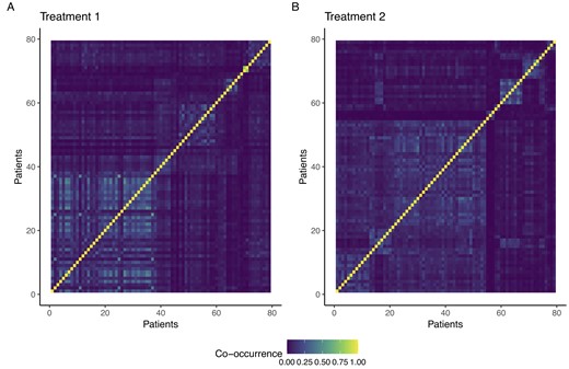
Heatmap of averaged co-occurrence matrix for patients who received Treatment 1 (pane A) and Treatment 2 (pane B).
To characterize the groups, we consider the cluster-specific mean for predictive biomarkers. Figure 2 shows that cluster-specific means in T1G2, T1G4, and T2G6 strongly depart from the population value. Moreover, T1G2 and T1G4 feature the underexpression of a mutual set of proteins, namely SF2, RB15, and KU80, still presenting opposite trends in the expression of AKT, YAP, BC2, and GSK3. Cluster-specific means in T2G1, T2G2, and T2G3 are really close for almost all the proteins. Noticeably, T2G3 features a sharp underexpression of AKT with respect to the mean values expressed in T2G1 and T2G2. Finally, patients in T2G6 show underexpression of SF2, AKT, RBM15, and KU80, in addition to the overexpression of GSK3. It is important to note that both T1G4 and T2G6 exhibit similar protein expression patterns. Specifically, both groups displayed underexpression of SF2, AKT, RBM, and KU80, as well as overexpression of GSK3. The role of these proteins in tumor progression is not entirely understood. Nonetheless, most of these proteins have been implicated in gliomas’ oncogenesis and developmental processes (Mills et al., 2011; Li et al., 2020). A better characterization of the groups of interest can be achieved by evaluating the cluster-specific response probability. To obtain meaningful cluster-specific parameters, we consider the a posteriori estimated clustering |$\hat{\mathcal {P}}^{a}_{n^a}$| as fixed, and—conditional on it—we obtain the a posteriori distribution of |$\boldsymbol \pi ^{a\star }_j$|s. Response probabilities are summarized by the posterior distributions |$\boldsymbol \pi _{j}^{a\star }\mid \hat{\mathcal {P}}^{a}_{n^a}, \boldsymbol x^a$| displayed in Figure 3.
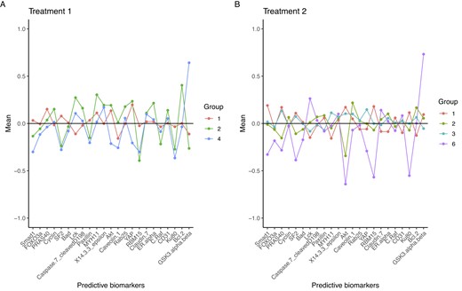
Group-specific mean of predictive biomarkers for patients who received Treatment 1 (pane A) and Treatment 2 (pane B).
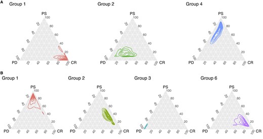
Ternary plot of the posterior density of group-specific response probabilities for patients who received Treatment 1 (row A) and Treatment 2 (row B).
Figure 3 displays the response probabilities for patients who underwent the standard treatment (row A). Patients in T1G1 are those who most benefit from the standard treatment, as the posterior distribution of the response probability is concentrated toward the CR vertex. On the other hand, patients in T1G4 and T1G2 are more likely to experience a partial or nonresponse to the treatment. Response probabilities for patients who received Treatment 2 (Figure 3, row B) clearly characterize these clusters of patients, too. Notably, the posterior densities exhibit an evident skewness toward the vertices of the ternary plot. If we consider T2G1, T2G2, and T2G3, our model successfully uses predictive biomarkers along with the response to the treatment to cluster patients. In fact, t-ppmx is able to distinguish between patients who may be similar in terms of their covariates (see 2, pane B) but have different responses to treatment, which is a common phenomenon in cancer genetics. Nonetheless, it is also important to notice that discrimination of respondents may be accomplished based on AKT protein underexpression. Among the Treatment 2 clusters, T2G6 is characterized by unique patterns in terms of posterior probabilities and cluster-specific means. On a comparative analysis, it is noteworthy that T2G6 and T1G4 exhibit a shared set of under/upregulated proteins, namely SF2, AKT, RBM15, and KU80 are underexpressed and GSK3 is overexpressed. Consequently, T1G4 and T2G6 subjects can be regarded as individuals with closely related genetic profiles who underwent different treatment modalities. Intriguingly, these patients have shown limited response to the standard procedure (Treatment 1), whereas they appear to be responsive to the advanced treatment (Treatment 2). Interpretation of the within-cluster expression levels needs particular care. Interactions among the proteins and the relationships between proteins’ expression and tumor progression are highly complex. Nonetheless, our analysis provides a proof of concept that the proposed method can empirically identify subgroups in heterogeneous populations. Noteworthy, the proposed method quantifies the group-specific deviation from a population baseline accounting for the variability in the clustering and, in contrast to what is typically done with regression models, does not require us to prespecify the functional form of the association between predictive covariates and the outcome variable.
8 DISCUSSION
We have proposed a novel Bayesian approach that, given a set of predictive and prognostic biomarkers, suggests the best-suited treatment for each patient. The model clusters patients into homogeneous groups with respect to their predictive markers, separately for each treatment. Cluster-level effects adjust the baseline probability of response to treatment obtained by prognostic factors. As a key innovative feature of the proposed approach, model-based clustering and treatment assignment are jointly estimated from the data, that is, treatment selection fully accounts for patients’ heterogeneity. Simulation studies and the analysis of LGG data showed that the proposed method is well suited for predictions in scenarios of practical relevance, for example, in the presence of considerable heterogeneity. Moreover, our approach leads to a precise characterization of the clusters of patients supported by the data, identifying the group of patients more likely to benefit from targeted treatments. In its current version, the model is designed to be used after the biomarker discovery phase, that is, after identifying relevant prognostic and predictive biomarkers. This limitation could be addressed by adopting variable selection approaches in the Bayesian framework. Nevertheless, while the use of the latter methods is straightforward when selecting prognostic biomarkers entering the likelihood, variable selection methods for PPMs are part of our ongoing research (see, for instance, Barcella et al., 2017). In this regard, we would like to highlight that, although assuming which are the prognostic and predictive biomarkers may be restrictive in certain scenarios, and we could recast the proposed model to accommodate this lack of knowledge, this assumption remains practically very relevant. In fact, the major drawback of a model that simultaneously performs biomarker discovery and treatment selection would be the absence of a confirmatory process. Biomarkers can lead to targeted therapy and serve as useful prognostic and predictive factors of clinical outcomes. Nonetheless, biomarkers need to be validated on a completely independent data set not used during development to serve these purposes.
Acknowledgments
We thank J. Ma for providing us with the companion R code of Ma et al. (2019).
Funding
The first and third authors were partially supported by the “Dipartimenti Eccellenti 2023-2027” ministerial funds (Italy). All authors were partially supported by the grant “CLUstering: Bayesian Partition Models for Precise Medicine (CluB: PMx2),” funded by Fondo di Beneficienza di Intesa San Paolo (Italy), and the last author was partially supported by the Tuscany Health Ecosystem (THE) grant, funded by Ministero dell’Università e della Ricerca.
Conflict of interest
None declared.
Data availability
The data that support the findings in this paper are available in the National Cancer Institute Genomic Data Commons (NCI GDC) data portal at https://portal.gdc.cancer.gov/. These data were derived from the following resources available in the public domain: https://portal.gdc.cancer.gov/projects/TCGA-LGG.
References
 Open Materials
