


Abstract
Survival models are used to analyze time-to-event data in a variety of disciplines. Proportional hazard models provide interpretable parameter estimates, but proportional hazard assumptions are not always appropriate. Non-parametric models are more flexible but often lack a clear inferential framework. We propose a Bayesian treed hazards partition model that is both flexible and inferential. Inference is obtained through the posterior tree structure and flexibility is preserved by modeling the log-hazard function in each partition using a latent Gaussian process. An efficient reversible jump Markov chain Monte Carlo algorithm is accomplished by marginalizing the parameters in each partition element via a Laplace approximation. Consistency properties for the estimator are established. The method can be used to help determine subgroups as well as prognostic and/or predictive biomarkers in time-to-event data. The method is compared with some existing methods on simulated data and a liver cirrhosis dataset.
1 INTRODUCTION
In medical research with survival outcomes, certain biomarkers may be associated with time to death, tumor progression, or other time-to-event measures. Understanding the relationship between biomarkers and survival is critical to optimizing patient treatment in a personalized medicine paradigm (Nalejska et al., 2014). Biomarkers that relate to survival independent of treatment are considered prognostic, whereas biomarkers that identify subgroups that are more likely to benefit from a treatment are considered predictive (Oldenhuis et al., 2008). Determining if a biomarker is prognostic or predictive requires assessing if there is a statistical interaction between the biomarker and treatment. In the rich literature of survival analysis, most methods are designed for either inference or prediction. In cases where a complex relationship between covariates and survival exists, simpler models that provide clear inference may not predict or estimate complexity adequately. When more sophisticated models capture the underlying complexity, understanding the interaction between variables and the impact on survival is more difficult, not because of the method itself, but because the underlying relationship of the data is complicated, and is difficult for humans to understand. The purpose of the method proposed in this paper is to provide methodological middle ground where inference and human interpretability are maintained without sacrificing predictive accuracy or oversimplifying the rich and complex nature of the data.
The Cox proportional hazard, accelerated failure time, and proportional odds models and their extensions are popular modeling tools to relate survival times with predictors or covariates in the presence of censorship. Bayesian analysis of survival data is popular due to its flexibility to include prior information, suitability to develop complex models, and ability to construct efficient algorithms for full scale uncertainty quantification (Sinha and Dey, 1997; Ibrahim et al., 2001). Bayesian semi-parametric regression models for survival data have been developed using the Gamma process, the Dirichlet process, and Polya tree priors and their mixtures (Kalbfleisch, 1978; Dykstra and Laud, 1981; Christensen and Johnson, 1988; Lo and Weng, 1989; Gelfand and Mallick, 1995; Kuo and Mallick, 1997; Walker and Mallick, 1999; Hanson and Johnson, 2002; Gelfand and Kottas, 2003; Ishwaran and James, 2004; Fernández et al., 2016). These popular models are constrained by parametric assumptions such as proportional hazards, constant odds, linearity, etc. Recently, several flexible Bayesian models have been developed to accommodate data complexities using dependent processes and their extensions (De Iorio et al., 2009; Jara and Hanson, 2011; Nieto-Barajas, 2014; Nipoti et al., 2018; Riva-Palacio et al., 2021).
Survival trees and forest-based models are popular non-parametric alternatives to semi-parametric models that can model non-linear interactions among variables and are easy to interpret. Tree-based survival analysis was introduced in the 1980s primarily through the extension of classification and regression tree (CART) models (Breiman et al., 1984) to censored survival data (Ciampi et al., 1981; Gordon and Olshen, 1985) and further extensions (LeBlanc and Crowley, 1993; Bou-Hamad et al., 2011). The major difference among these papers is the use of different splitting criteria such as log-rank statistics, likelihood ratio statistics, Wilcoxon-Gehan statistics, node deviance measures, and impurity measures. A crucial issue of these tree models is the selection of a single tree of suitable size using forward or backward algorithms. The Bayesian classification and regression tree methods were developed by Chipman et al. (1998) and Denison et al. (1998), with others such as Clarke and West (2008) proposing extensions. Bayesian additive regression trees (BART) introduced by Chipman et al. (2010) have become the basis for the majority of Bayesian survival tree-based models (Kalbfleisch, 1978; Bonato et al., 2010; Sparapani et al., 2016, 2023; Henderson et al., 2017, 2020; Linero et al., 2022).
In contrast to ordinary learning approaches which construct 1 learner from training data, ensemble methods construct a set of learners known as base learners and combine them for prediction. Base learners are usually generated from the training data by a standard algorithm like decision trees, neural networks, or other kinds of learning algorithms. There are 2 major kinds of ensemble methods based on the method of construction of the base learners. The first type is sequential ensemble methods where the base learners are generated sequentially and the dependence among these base learners are used efficiently, such as AdaBoost (Freund and Schapire, 1997). The alternative type of ensemble learning constructs the base learners in a parallel way, as is done in bagging (Breiman, 1996). Recently, ensemble trees (Ishwaran et al., 2004, 2008; Hothorn et al., 2005, 2006; Zhou et al., 2015; Hothorn and Zeileis, 2017) have become a popular alternative as a predictive survival model building tool using the concepts of bagging and random forests (Breiman, 1996, 2001). Even though machine learning algorithms usually focus on the predictive performance, research in the field of interpretable machine learning (Doshi-Velez and Kim, 2017; Molnar, 2020) has flourished due to its direct connection with artificial intelligence (Kuziemsky et al., 2019). However, a black-box machine-learning based predictive tool is not sufficient in many cases, such as medical research, and a more interpretable decision system is needed. Hence, most of the ensemble methods, based on boosting (Lee et al., 2021) or bagging logic, are not suitable in this framework.
We propose an interpretable and flexible machine-learning model for survival data. Similar to the original CART papers, a single tree model is used, which is simple to interpret. The proposed model moves beyond proportional hazards (Cox, 1972) and is different than existing CART models where simple parametric models (like Gaussian or multinomial models) with conjugate priors have been used at the terminal nodes of the tree. Instead, we model the unknown log-hazard function at each terminal node of the tree with a Gaussian process, which is flexible but results in a non-conjugate posterior distribution. In this setup, obtaining the marginal likelihood analytically is not possible, which is a key step of the existing Bayesian tree search algorithms for CART as well as BART models. The approximate posterior of trees is efficiently searched via Markov chain Monte Carlo (MCMC) by obtaining the marginal likelihood of the observed data via a Laplace approximation (Tierney and Kadane, 1986). The combination of interpretability coupled with flexibility makes this model well-suited for many problems, including subgroup identification and identifying prognostic and predictive biomarkers in medical research. In general, this new approach will allow the Bayesian tree models to be applied in more complex modeling scenarios. Moreover, an important contribution of this paper is to establish posterior consistency properties for the estimator.
2 SURVIVAL MODELS
Let t be a continuous non-negative random variable representing survival time with density function p(t), survival function S(t), and hazard function h(t) = p(t)/S(t). In general, the hazard function depends on the survival time and the vector of covariates |$\mathbf {x}=(x_{1},x_{2},\ldots ,x_{d_0})$|. The Cox proportional hazards model (Cox, 1972) allows time and covariates to affect the hazard function separately, |$h(t \mid \mathbf {x})=h_{0}(t){\rm exp}(\mathbf {x}\boldsymbol{ \beta })$|, where h0 is the baseline hazard and |$\boldsymbol{ \beta }$| is a vector of regression parameters. This model has a strong assumption that the ratio of hazards for 2 individuals depends on the difference between their linear predictors at any time.
We extend this class of models by developing the Treed Hazards Model (THM). In the THM, we split the covariate space of x with tree partitions and a fit a Gaussian process model to the log-hazards within each partition element. Let’s denote the tree as T with |$\#(T)$| terminal nodes and the vector of hazards within tree partition elements (terminal nodes) as |$\mathbf {h}=[h_{1}(\cdot),h_{2}(\cdot),\ldots ,h_{\#(T)}(\cdot)]$|, where hi(·) is the hazard function at the ith terminal node. This is in contrast to specifying a conjugate model at each terminal node as in existing Bayesian CART models. The THM describes the conditional distribution of t given x in this tree structure. If x lies in the region corresponding to the ith terminal node then t∣x has the distribution p[t∣hi(·)]. In the next section, we develop the hierarchical tree model for the survival data.
2.1 The Bayesian hierarchical treed hazards model
Let y = {|$y_1 , \ldots , y_n$|} be the survival time for n subjects (realizations of t), |$\boldsymbol{ \delta }= \lbrace \delta _1, \ldots , \delta _n\rbrace$| be the corresponding censoring indicators, where δj is 1 if yj is observed and 0 if yj is right censored. Then, we can write the posterior distribution of the model unknowns T and h as |$p(T,\mathbf {h}\mid \mathbf {y},\mathbf {x},\boldsymbol{ \delta })\propto p(\mathbf {y}, \boldsymbol{ \delta }\mid T,\mathbf {h})\pi (\mathbf {h}\mid T)\pi (T \mid \mathbf {x})$|. In the following sections, we specify the likelihood function |$p(\mathbf {y}, \boldsymbol{ \delta }\mid T,\mathbf {h})$| and the prior distributions π(h ∣ T) and π(T ∣ x).
2.1.1 Tree partition and the prior distribution π(T ∣ x)
First, we describe the tree partition T on the covariate space and the related prior distribution. We assume that the data can be partitioned into |$\#(T)$| partition elements |$\mathbf {y}_1,\ldots ,\mathbf {y}_{\#(T)}$|, such that |$\bigcup _{i=1}^{\#(T)} \mathbf {y}_i = \mathbf {y}$| and |$\mathbf {y}_i \cap \mathbf {y}_{i^\prime } = \emptyset$| for all i ≠ i′. We further assume that, for a given tree T, the data within the ith partition element are conditionally independent given the hazard function, hi(t), and assume that the |$\#(T)$| hazard functions are mutually independent. The tree partition is constructed through a series of recursive binary splits of the covariate space (Chipman et al., 1998). The binary tree T subdivides the predictor space marginally by choosing one of the d0 covariates from x and then defining a partition rule.
We adopt the same prior as Chipman et al. (1998), which is constructed by splitting the tree nodes with a designated probability and assigning a rule each time a node is split. Let |$S_{i^\prime }$| equal 1 if the i′th node is split, otherwise 0, |${i^\prime }=1,\ldots ,2\#(T)-1$|. Let |$R_{j^\prime }= (v_{j^\prime },r_{j^\prime })$|, |${j^\prime }=1,\ldots ,\#(T) - 1$| represent the rules of the |$\#(T) -1$| internal nodes. Here, |$v_{j^\prime }\in \lbrace 1,\ldots ,d_0\rbrace$| indicates which variable is to be split, and |$r_{j^\prime }$| is the splitting rule on the |$v_{j^\prime }$|th variable. The partition rule for continuous variables is formed by choosing a threshold and then grouping observations based on whether or not their covariate value is less than or equal to, or greater than, the splitting threshold. For categorical variables, the split rule is defined as a subset of the unique categories for that variable, and observations are grouped based on whether their covariate value is in the subset or not.
Let |$T = (S_1,\ldots ,S_{2\#(T) -1},R_1,\ldots ,R_{\#(T)-1})$| be the collection of split indicators and rules for a particular tree. Then the prior for a tree, T, can be evaluated as
Following Chipman et al. (1998), we define |$\pi (S_{i^\prime }= 1) = 1 - Pr(S_{i^\prime }= 0) = \gamma (1 + d_{i^\prime })^{-\theta }$| where |$d_{i^\prime }$| represents the depth of the i′th node (ie, the root node has a depth of 0, child nodes of the root node have depth 1, etc.). Here, γ and θ are hyperparameters chosen by the modeler and influence the prior for the general size and shape of the tree. Here, |$\pi (R_{j^\prime }) = 1/(m_{j^\prime }m^\star _{\nu _{j^\prime }})$| where |$m_{j^\prime }$| represents the number of variables on the corresponding node that are available for splitting and |$m^\star _{\nu _{j^\prime }}$| is the number of splitting rules available on the selected variable for the node to which the rule belongs. The splitting rules at a given node are selected from the observed data, which reach that node from its ancestry.
2.1.2 The likelihood function |$p(\mathbf {y}, \boldsymbol{ \delta }\mid T,\mathbf {h})$|
The partition model assumes that given a tree, T, the hazard functions at each terminal node are independent and the data within a terminal node, given the hazard function at the node, are independent and identically distributed. It is important to note that covariates are used to construct the tree, T, but are not used in the hazard functions. Consequently, the likelihood function, given a tree, can be expressed as a simple product of likelihoods, |$p(\mathbf {y}, \boldsymbol{ \delta }\mid T, \mathbf {h}) = \prod _{i=1}^{\#(T)} p[\mathbf {y}_i, \boldsymbol{ \delta }_i \mid h_i(\cdot)]$|, where |$\mathbf {y}_i,\ \boldsymbol{ \delta }_i$| represent the ni responses and censoring indicators, which belong to the ith terminal node, |$p[\mathbf {y}_i, \boldsymbol{ \delta }_i \mid h_i(\cdot)]$| represents the likelihood of |$\mathbf {y}_i,\ \boldsymbol{ \delta }_i$| given the hazard function in the ith terminal node and |$\#(T)$| is the total number of terminal nodes.
2.1.3 Hazard prior and the data-generating density
We write the density of an uncensored observation at the ith terminal node as |$p_i(t)=h_i(t)e^{-\int _0^th_i(s)ds}$| for hazard function hi(·). Let pc(·) be the density of the censoring distribution, which has the same support as the true densities for the uncensored observations.
We place a Gaussian process prior on the log-hazard rate function on [0, Ln], where Ln = max {yi}, log hi(·) = wi(·), and wi(t) follows a Gaussian process with covariance function |$\tau _i^2K(\frac{s}{l_i},\frac{t}{l_i})=\tau _i^2\exp \lbrace -|s-t|/l_i\rbrace$|, and let |$\pi (\tau _i^2,l_i)=\pi (\tau _i^2)\pi (l_i)$| be the prior on the hyperparameters. For a generic partition |$\mathscr {P}=\lbrace P_1,\dots , P_{k^{\prime }}\rbrace$| of the covariate space and the partition densities pi(·), for observation y, x, and the censoring indicator function δ, the data-generating density p(·) is given by under the assumption of random censoring,
We observe (y1, δ1)|$, \ldots ,$| (yn, δn) at observed covariates |$\boldsymbol {\rm x}_1 , \ldots , \boldsymbol {\rm x}_n$|, where xj are i.i.d. for j = |$1 , \ldots , n$|. Let |$\#(T)$| denote the number of partitions/terminal nodes for a tree T. Denoting the generic prior distribution by π(·), the prior for the treed hazards model is
2.1.4 Approximate posterior, Laplace approximation, and MCMC
In practice, the Gaussian process prior on the log-hazard is evaluated on a finite grid and the log-hazard is assumed piecewise constant. Furthermore, by utilizing a Laplace approximation, the approximate posterior of the tree, T, can be obtained as |$\tilde{p}(T \mid \mathbf {y}, \boldsymbol{ \delta }, \mathbf {x})$|, which can be searched effectively through a reversible-jump MCMC algorithm (Green, 1995), similar to Payne et al. (2020). Details are provided in Web Appendix 1.
3 CONSISTENCY RESULTS
In this section, we show the density estimation consistency when the true data-generating density follows a partition model induced by a tree. If the survival function for the true data-generating density has a tree partition form, then first we show that as n, the number of observations goes to infinity, the posterior distribution concentrates on any weak neighborhood of the true data-generating density with probability 1. Later, we show the consistency under model misspecification for Lipschitz continuous log-hazard functions, and also misspecification of the tree structure. Then under slightly stronger conditions, we establish the L1 consistency. Some of the details and the proofs are relegated to Web Appendix 2of the supporting materials.
Let |$P_1^{*},\dots ,P_{m^{*}}^{*}$| be the true partition of the covariate space denoted as |$\mathscr {P}^{*}=\lbrace P^{*}_1,\dots ,P_{m^{*}}^{*}\rbrace$|, and let h0, i(t) > 0, t > 0 for i = |$1 , \ldots , m^*$|, be the true hazard function for partition |$P_i^{*}$| and the corresponding true uncensored data-generating density for the ith partition is given by |$p_{0,i}(t)=h_{0,i}(t)e^{-H_{0,i}(t)}$| where |$H_{0,i}(t)=\int _0^th_{0,i}(s)ds$|. As mentioned earlier, pc is the density of the censoring distribution. We assume that the p0, i(t)’s have the same support. Let Fc and F0, i be corresponding cdfs and |$1-F_{0,i}(t)=e^{-H_{0,i}(t)}$|.
We discuss the conditions needed for our result to hold. The conditions [A1] through [A6] are given in supporting materials (Supporting Material; Web Appendix 2) and discussed in the following. We first need conditions [A1] and [A3] to ensure the Reproducing Kernel Hilbert Space (RKHS) support condition for the Gaussian process, given by |$\log (h_{0,i}(t))=\int _{R_Y} \tilde{g}_i(s)K(s/l_i^{*},t/l_i^{*})ds$|, for some bounded, Lipschitz-continuous and integrable functions |$\tilde{g}_i$|’s and RY is the range of the p0, i(·)’s.
We also need a uniform upper bound for the moment under density functions of the p0, i(·)’s, and pc(·) (condition [A2]), and an exponentially decaying tail condition (given in [A5]). We assume the covariates are uniformly bounded, and the continuous covariate is partitioned into mn equi-spaced grids for the tree splitting rule. The details and related prior conditions are given in condition [A4], and the conditions needed for hyper-parameters are given in condition [A6]. Conditions [A1], [A4], [A5], and [A6] guarantee enough prior probability in a small neighborhood around the true data-generating density under the partition-tree model.
Suppose the true partition |$\mathscr {P}^{*}$| is achieved for a tree |$T^*$|, and let |$\hat{\mathscr {P}}^{*}=\hat{\mathscr {P}}_T^{*}=\lbrace \hat{P}_l^{*}:l=1,\ldots ,m^{*}\rbrace$| corresponding to |$T=\hat{T}^{*}$| be an approximating partition, with |$\hat{T}^{*}$| having the same number of terminal nodes as in |$T^*$|. We define the following distance between these 2 partitions by |$d(\mathscr {P}^{*},\hat{\mathscr {P}}^{*})=\text{min}_{c(1),\dots ,c(m^{*})} \sum _{i=1}^{m^{*}}\mu _x(P_i^{*}\Delta \hat{P}_{c(i)}^{*})$|, where |$c(1), \ldots , c(m^*)$| is a permutation of |$1,\ldots ,m^{*}$|, and μx is the measure associated with the covariate space.
For any bounded continuous function g, and for ϵ > 0, let |$U^{\epsilon }_g=\lbrace p:|\int g p^{*}(\cdot)-\int g p(\cdot)|\lt \epsilon \rbrace$|, be a weak neighborhood of the true joint density |$p^*(\cdot)$|. Under the model in Equation 2, prior in Equation 3, under assumptions [A1] through [A6] in supporting materials, and under the true data-generating distribution |$p^*$|, |$\Pi _n(U^{\epsilon }_g\mid \cdot)\rightarrow 1$| almost surely, as n → ∞, where Πn|$(\cdot \mid \cdot)$| denotes the posterior distribution based on n observations.
Theorem 1 establishes consistency in weak topology, with Πn|$(\cdot \mid \cdot)$| being weakly consistent at |$\lbrace {p_{0,i}}_{i=1,\ldots ,m^{*}},p_c,\mathscr {P}^{*} \rbrace$|. Even though we state Theorem 1 under the support condition given in [A3], the consistency result will hold true for more general support under additional mild conditions, given in the following. Theorem 1 does not assume piecewise-constant hazard functions, and guarantees posterior mass concentrating in a weak ϵ-neighborhood around the true data-generating density, which we approximate by piecewise constants. However, the result holds for piecewise constant (in time) densities under [A1] through [A6].
Theorem 1 holds for piecewise constant hazard functions, which eventually converges to a constant that is log h0, i(t) = c0, i for t ≥ T0, i ≥ 0 for i = |$1,\ldots ,m^{*}$|, if we assume |$c_0l_i^{\alpha _{0,i}}\le \pi (l_i)$| for some α0, i > 0, c0 > 0 for |li| ≤ cl, cl > 0.
Theorem 1 holds for bounded Lipschitz continuous log h0, i(t)’s, if we assume |$c_0l_i^{\alpha _{0,i}}\le \pi (l_i)$| for some α0, i > 0, c0 > 0 for |li| ≤ cl, cl > 0.
If the true partition is not induced by a tree, but given any ϵ > 0, can be approximated by a partition |${\mathscr {P}}_1^{*}$|, induced by a tree |${T}_1^{*}$| (where |${T}_1^{*}$| may depend upon ϵ), such that |$d(\mathscr {P}^{*},{\mathscr {P}}_1^{*})\lt \epsilon$|, then Theorem 1 holds.
General Misspecification. Suppose we have bounded true log-hazard function log h0(x, t), that is, Lipschitz continuous in covariate x and t for continuous covariates. If we assume that the categorical covariates have finite ranges, and for continuous covariates the density functions are bounded away from 0 and infinity, then, the log-hazard function can be approximated by THM, and the result of Theorem 1 will hold for prior condition on li’s given in Remarks 1 and 2, and the posterior probability of |$U^{\epsilon }_g$| will approach 1 almost surely, as n approaches infinity.
Proof of the Remarks 1 through 4 are given in Web Appendix 2. Performance of THM under model misspecification can be seen in the example in Section 4.1. For the strong consistency, we consider estimated densities and show that they will remain in a small L1 neighborhood of the true density with probability 1. We assume additional conditions [B1] through [B5] (given in Web Appendix 2 of the supporting materials).
Let ϵ > 0 and |$U^{\epsilon}=\lbrace p:\int |p^{*}(\cdot)-\int p(\cdot)|\lt \epsilon \rbrace$|, be an L1 neighborhood of the true joint density |$p^*(\cdot)$|. Under the model in Equation 2 and related prior distributions, under assumptions [A4], [B1] through [B5] in supporting materials, and under the true data-generating distribution |$p^*$|, Πn(U ϵ ∣ ·) → 1 almost surely as n → ∞.
As described in Section 2.1.4, the THM is implemented by evaluating the log-hazard Gaussian process on a finite grid and utilizing a Laplace approximation. Although it is beyond the scope of this paper to address the impact of the Laplace approximation on consistency directly, Section 4 assesses the performance of the THM via simulation to provide empirical evidence of its effectiveness in practice.
4 SIMULATIONS AND APPLICATIONS
4.1 Prognostic and predictive biomarker
Identifying predictive and prognostic biomarker effects is important in drug development. Sometimes there is a hypothesis that a certain sub-population, based on a predictive biomarker, will respond better to a treatment. Other times, the value of a prognostic biomarker is related to a patient’s prognosis. It is possible a biomarker may be both prognostic and predictive.
A single biomarker, b, and a treatment assignment indicator, a (0 for placebo, 1 for treatment), are simulated in 50 datasets, each with 1 000 observations. The biomarker is constructed to be both prognostic and predictive. The time to event, y, is simulated from a Weibull model with an average random right-censoring rate of 27% with a ∼ Binomial(1, .5), b ∼ Uniform(0, 1), y ∼ Weibull(1 + 2ab, 1 + 5b), where Weibull(λ, k) is a Weibull distribution with scale λ and shape k. For small biomarker values b nearer to 0, there is a small treatment effect, whereas for values of b closer to 1, there is a large treatment effect, thereby creating a predictive biomarker. For a fixed treatment assignment a, the shape of the survival curve is a function of b, creating a prognostic effect for the biomarker.
The simulated datasets were fit with the THM, a frequentist Cox proportional-hazard model with a non-parametric baseline hazard and an interaction between a and b, Bayesian additive regression trees (Sparapani et al., 2016), and survival random forests (Ishwaran et al., 2008). For each simulation, an additional independent dataset was generated on which Brier scores (Graf et al., 1999) were calculated at the 10th, 25th, 50th, 75th, and 90th percentiles marginally over a and b. For THM, the tree with the highest posterior probability was used in the calculations. Note that due to the flexible nature of THM, it is unable to extrapolate. Therefore, to ensure a clear comparison between methods, the independent dataset on which Brier scores are calculated is subset to observations where a valid estimate of the survival function can be obtained from the THM at a given percentile. This primarily affects the calculations for the 75th and 90th percentiles, where some of the independent data may fall outside the range of the data used to fit the THM. The Brier scores from the 50 simulations are shown in Figure 1 and show no significant differences between the BART, Forest, and THM methods, whereas the Cox method has worse (higher) Brier scores across all percentiles, likely because the proportional hazard assumption is too restrictive. This is problematic—even if the Cox model identifies a significant treatment by biomarker interaction, which is often used to determine a predictive biomarker effect, the estimates of the survival curve may be inaccurate.
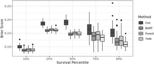
Brier scores at different survival percentiles (marginalized over treatment a and biomarker b) for the simulated datasets in the predictive/prognostic simulation.
On the other hand, BART, random forests, and THM can both identify important variables and estimate survival more accurately. However, in some fields, such as medical research, it is not enough to know that variables marginally predict survival—it is also important to know if and how these variables interact, for example, in order to identify if specific subgroups may be more likely to respond to treatment. In BART and random survival forests, this requires manual exploration of survival curves throughout the covariate space to better understand which predictors are prognostic, predictive, or both. In contrast, the THM automatically provides both accurate estimation and clear interpretation. Figure 2 displays the tree with the highest posterior probability from one of the simulations with the posterior mean and 95% credible intervals of the survival curves at each of the terminal nodes. The prognostic nature of the biomarker can be seen on the left side of the tree, which indicates that, regardless of treatment, the biomarker influences the survival curve shape. On the right side of the tree, the predictive nature of the biomarker becomes evident: as the biomarker increases, survival in the treatment arm improves.
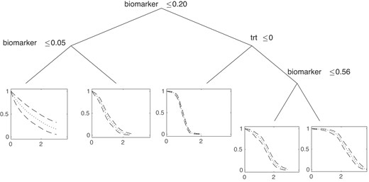
Tree with the highest posterior probability from one of the predictive/prognostic simulations. The posterior mean (dotted) and 95% credible intervals (dashed) of the survival curve is shown at each terminal node.
4.2 Analysis of primary biliary cirrhosis data
Primary biliary cirrhosis survival data collected from 1974 to 1984 by the Mayo Clinic and obtained via the R survival package (Therneau, 2020) were fit using the THM. Covariates included treatment group (D-penicillamine or placebo), age, sex, edema status (0 no edema, 0.5 untreated or successfully treated, 1 edema despite diuretic therapy), serum bilirunbin (mg/dl), serum albumin (g/dl), and standardized blood clotting time. Only subjects who were randomized to treatment and had no missing values were included in the analysis yielding a total of 276 subjects in the analysis. The outcome of interest was time to death, and patients were censored at the end of study or if they received a transplant, yielding a censoring rate of 60%.
Ten thousand MCMC samples were drawn and the tree with the highest posterior probability is shown in Figure 3. The posterior mean and 95% credible intervals from the THM and the Kaplan-Meier curves are overlayed at each terminal node and indicate the THM is very flexible and similar to the Kaplan-Meier estimates.
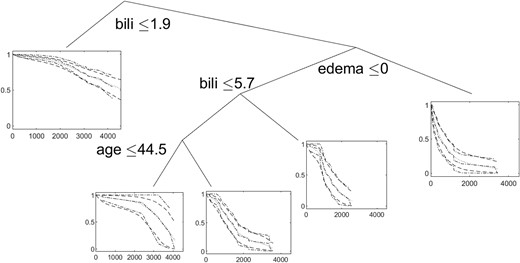
The tree with the highest posterior probability and the posterior mean (dotted), 95% credible intervals (dashed), and the Kaplan-Meier estimates (dash-dotted) at each terminal node.
The tree indicates that patients with bilirubin levels ≤1.9 have the highest survival rates. For subjects with no edema and bilirubin levels >1.9 and less than or equal to 5.7, patients under the age of 45 had better survival. Patients with bilirubin levels >1.9 and edema had the worst survival. These conclusions are consistent with the findings of Dickson et al. (1989), who used a Cox proportional hazards model on primary biliary cirrhosis data; however, the tree method provides greater flexibility in estimating the survival curves, especially in this case where the hazards are not proportional. Last, we note that the tree did not split on treatment status, which is consistent with the findings of Gong et al. (2004), who performed a systematic review of the effect of D-penicillamine on patients with primary biliary cirrhosis and concluded that it does not decrease the risk of mortality.
To further assess the fit of the THM, k-fold cross-validation was performed with 10-folds on the THM, BART, random forest, and Cox models. The Brier scores at 5 percentiles of the empirical survival curve (marginalized over the covariates) are plotted in Figure 4. The THM, using a single tree with the highest posterior probability, had slightly higher observed mean Brier scores than BART and random forest. This is likely due to the smaller sample size of this dataset compared to the simulations in Section 4.1, where the methods performed similarly. The Cox model was generally worse than the 3 other models at the 10th and 50th percentiles, but was comparable at the 25th, 75th, and 90th percentiles. The lack of performance in the Cox model may be partially explained by a violation of proportional hazards, which is evident from the various survival curve shapes in Figure 3.
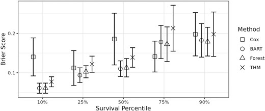
Mean Brier scores with 95% confidence intervals at different percentiles (marginalized over the covariates) of the survival curve from 10-fold cross-validation for the primary biliary cirrhosis data.
5 DISCUSSION AND CONCLUSION
One of the main intentions of the THM is to enhance interpretability while maintaining flexibility. To that end, it is not intended to be used with a large number of covariates. A very large number of covariates may reduce the overall human-interpretability of the trees, as well as make it difficult for the MCMC to adequately explore the posterior of the trees. Ideally, a few important variables may be determined through other methods, and the THM may then be applied to provide meaningful interpretation of the most important variables.
Although this paper has focused on making inference on the tree with highest posterior probability, in practice, multiple trees near the maximum posterior probability tree estimate from the MCMC should be viewed to determine how consistent the top trees are in their partitioning. If most of the top trees partition the covariate space in a very similar way, then more confidence can be given to the inference. Conversely, if there are several trees that partition the covariate space quite differently, it indicates there is more uncertainty regarding a partitioning structure, and the results of several trees should be considered.
The main advantage of the treed hazards model is its ease in interpretation coupled with its flexibility. Inference is easily obtained from inspecting posterior trees to understand how survival curves are influenced by covariates, which can help identify prognostic and predictive biomarkers in medical research. In both simulations and applications, the model performs well in identifying interpretable partitions and flexibly estimating and predicting survival curves as evidenced by Brier scores. Furthermore, we have established weak consistency for the partition model under the proposed kernel, where we can accommodate flexible forms of the hazard function under moderate conditions.
Acknowledgement
The authors R.D.P. and N.G. contributed equally to this paper. The authors would like to thank the associate editor and 2 anonymous referees, whose comments greatly improved the presentation of the material in this paper.
FUNDING
N.G. is partially supported by the National Science Foundation grant: NSF DMS #2015460.
B.K.M. is partially supported by the National Science Foundation grant: NSF CCF-1934904.
CONFLICT OF INTEREST
None declared.
DATA AVAILABILITY
The data underlying this article are available in the R survival package (Therneau, 2020), which can be obtained through the Comprehensive R Archive Network at https://cran.r-project.org/package=survival.
