


Abstract
Biomedical research now commonly integrates diverse data types or views from the same individuals to better understand the pathobiology of complex diseases, but the challenge lies in meaningfully integrating these diverse views. Existing methods often require the same type of data from all views (cross-sectional data only or longitudinal data only) or do not consider any class outcome in the integration method, which presents limitations. To overcome these limitations, we have developed a pipeline that harnesses the power of statistical and deep learning methods to integrate cross-sectional and longitudinal data from multiple sources. In addition, it identifies key variables that contribute to the association between views and the separation between classes, providing deeper biological insights. This pipeline includes variable selection/ranking using linear and nonlinear methods, feature extraction using functional principal component analysis and Euler characteristics, and joint integration and classification using dense feed-forward networks for cross-sectional data and recurrent neural networks for longitudinal data. We applied this pipeline to cross-sectional and longitudinal multiomics data (metagenomics, transcriptomics and metabolomics) from an inflammatory bowel disease (IBD) study and identified microbial pathways, metabolites and genes that discriminate by IBD status, providing information on the etiology of IBD. We conducted simulations to compare the two feature extraction methods.
Introduction
Biomedical research now commonly integrates diverse data types (e.g. genomics, metabolomics, clinical) from the same individuals to better understand complex diseases. These data types, whether measured at one time point (cross-sectional) or multiple time points (longitudinal), offer diverse snapshots of disease mechanisms. Integrating these complementary data types provides a comprehensive view, leading to meaningful biological insights into disease etiology and heterogeneity.
Inflammatory bowel disease (IBD), including Crohn’s disease and ulcerative colitis, is a complex disease with multiple factors (including clinical, genetic, molecular, and microbial levels) contributing to the heterogeneity of the disease. IBD is an autoimmune disorder associated with inflammation of the gastrointestinal tract (Crohn’s disease) or the inner lining of the large intestine and rectum (ulcerative colitis), and is the result of imbalances and interactions between microbes and the immune system. To better understand the etiology of IBD, the integrated human microbiome project (iHMP) for IBD was initiated to investigate potential factors contributing to heterogeneity in IBD [1]. In that study, individuals with and without IBD from five medical centers were recruited and followed for one year and the molecular profiles of the host (e.g. host transcriptomics, metabolomics, proteomics) and microbial activities (e.g. metagenomics, metatranscriptomics) were generated and investigated. Several statistical, temporal, dysbiosis and integrative analyses methods were performed on the multiomics data. Integrative analyses techniques used included lenient cross-measurement type temporal matching and cross-measurement type interaction testing.
Our work is motivated by the IBD iHMP study and the many biological research studies that generate cross-sectional and longitudinal data with the ultimate goal of rigorously integrating these different types of data to investigate individual factors that discriminate between disease groups. Several methods, both linear [2, 3] and non-linear [4–6], have been proposed in the literature to integrate data from different sources but these methods expect the same types of data (e.g. cross-sectional data only, or longitudinal data only), which limits our ability to apply these methods to our motivating data that is a mix of cross-sectional and longitudinal data. For instance, methods for associating two or more views (e.g. [2, 3], iDeepViewLearn [7], JIVE [8], DeepCCA [4], DeepGCCA [9], kernel methods [10], co-inertia [11]) or for joint association and prediction (e.g. SIDA [12], DeepIDA [13], JACA [14], MOMA [15], CVR [16], randmvlearn [10], BIP [17], sJIVE [18]) are applicable to cross-sectional data only. The Joint Principal Trend Analysis (JPTA) method proposed in [19] for integrating longitudinal data is purely unsupervised, only applicable to two longitudinal data, cannot handle missing data and assumes the same number of time points in both views. However, methods for integrating cross-sectional and longitudinal data are scarce in the literature. The few existing methods [20, 21] do not maximize the association between views and, more importantly, when applied to our motivating data, cannot be used to identify variables discriminating between those with and without IBD. These methods use recurrent neural networks to extract features from different modalities and then simply concatenate the extracted features to perform classification.
To bridge the gap in existing literature, we build a pipeline that (1) integrates longitudinal and cross-sectional data from multiple sources such that there is maximal separation between different classes (e.g. disease groups) and maximal association between views; and (2) identifies and ranks relevant variables contributing most to the separation of classes and association of views. Our pipeline combines the strengths of statistical methods, such as the ability to make inference, reduce dimension and extract longitudinal trends, with the flexibility of deep learning, and consists of i) variable selection/ranking, ii) feature extraction, and iii) joint integration and classification (Fig. 1).
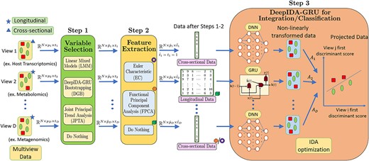
Pipeline for multiview data integration/classification. Variable selection: Every view’s data |$\mathbf{X}_{d} \in \mathbb{R}^{N \times p_{d} \times t_{d}}$| is first passed through this step to obtain |$\widetilde{\mathbf{X}}_{d} \in \mathbb{R}^{N \times \tilde{p}_{d} \times t_{d}}$|, where |$\tilde{p}_{d} < p_{d}$| if either LMM, DGB or JPTA is used for variable selection and |$\tilde{p}_{d} = p_{d}$| if this step is skipped. LMM focuses on selecting variables maximally separating the classes whereas JPTA focuses on those maximally associating the views. DGB focuses on identifying variables simultaneously maximizing within-class separation and between-view associations. LMM considers each variable separately and lacks context from other views and other variables within the same view. JPTA and DGB leverage between-view and between-variable relationships while selecting variables. JPTA works with two longitudinal views, whereas DGB is capable of taking in any number of views. Moreover, unlike JPTA, both LMM and DGB associate ranking with selected variables. Feature extraction: Feature extraction is performed on longitudinal views to convert |$\widetilde{\mathbf{X}}_{d} \in \mathbb{R}^{N \times \tilde{p}_{d} \times t_{d}}$| into |$\widehat{\mathbf{X}}_{d} \in \mathbb{R}^{N \times \hat{p}_{d} \times \hat{t}_{d}}$|, where |$\hat{t}_{d} =1$| if either EC or FPCA is used and |$\hat{t}_{d} = t_{d}$| if this step is skipped. EC and FPCA convert longitudinal data to one-dimensional form, which is especially important when one want to use the existing integration methods based on cross-sectional views only. EC outperforms FPCA when there are distinct differences in the covariance structure between the classes, while FPCA is better when there are variations in time-trends between the classes. Integration/classification: DeepIDA-GRU is used for integration/classification, where the longitudinal views are fed into GRUs and the cross-sectional views are fed into dense neural networks. The output of these networks are integrated using IDA and classified using Nearest Centroid Classifier.
In particular, for variable selection/ranking, we consider the linear methods (linear mixed models [LMM] and JPTA) and the nonlinear method (deep integrative discriminant analysis [DeepIDA] [13]). DeepIDA is a deep learning method for joint association and classification of cross-sectional data from multiple sources. It combines resampling techniques, specifically bootstrap, to rank variables based on their contributions to classification estimates. Since DeepIDA is applicable to cross-sectional data only, for longitudinal data, we combine DeepIDA with gated recurrent units (GRUs), a class of recurrent neural networks (RNN), to rank variables. We refer to this method as DeepIDA-GRU-Bootstrapping (DGB). Of note, LMM explores linear relationships between a longitudinal variable and an outcome and focuses on identifying variables discriminating between two classes; JPTA explores linear relationship between two longitudinal views and focuses on identifying variables that maximally associate the views; and DGB models nonlinear relationships between classes and two or more longitudinal and cross-sectional data and focuses on simultaneously maximizing within-class separation and between-view associations. For feature extraction, we explore the two methods: Euler characteristics (EC) and functional PCA (FPCA), to extract |$1$|-dimensional embeddings from each of the (|$2$|-dimensional) longitudinal views. EC and FPCA inherently focus on different characteristics of longitudinal data while extracting features and in this work, the two are compared and analysed using a simulated dataset. Finally, for integration and classification, we combine the existing DeepIDA method (without bootstrap) with GRUs, taking as input the selected variables and the extracted features from each view. Since we do not implement variable ranking at this stage, we refer to this method as DeepIDA-GRU, to distinguish it from DBG which implements bootstrap in DeepIDA with GRUs. DeepIDA-GRU could be used to integrate a mix of longitudinal and cross-sectional data from multiple sources and discriminate between two or more classes. We emphasize that DeepIDA-GRU combines the existing DeepIDA method (without bootstrap) with GRUs. As such, DeepIDA-GRU can directly take longitudinal data as input, making the feature extraction step (which could potentially lead to a loss of information) optional. Please refer to Fig. 1 for a visual representation of the DeepIDA-GRU framework.
In summary, we provide a pipeline that innovatively combines the strengths of existing statistical and deep learning methods to rigorously integrate cross-sectional and longitudinal data from multiple sources for deeper biological insights. Our pipeline offers four main contributions to the field of integrative analysis. First, our framework allows users to integrate a mix of cross-sectional and longitudinal data, which is appealing and could have broad utility. Second, we allow the use of a clinical outcome in variable selection or ranking. Third, we model complex nonlinear relationships between the different views using deep learning. Fourth, our framework has the ability to accommodate missing data.
Materials and methods
Datasets and data preprocessing
To evaluate the effectiveness of the proposed pipeline, we use simulations to compare the two feature extraction methods and make recommendations on when each is suitable to use. We applied the pipeline to cross-sectional (host transcriptomics data) and longitudinal (metagenomics and metabolomics) IBD data [1] from 90 subjects who had the three measurements. Before preprocessing, the metagenomics data contained path abundances of |$22113$| gene pathways, the metabolomics data consisted of |$103$| hilic negative factors, and the host transcriptomics data consisted of |$55\,765$| probes. We note that, for most of the participants, multiple samples of their host transcriptomics data were collected in a single week. Therefore, in this work, we consider the host transcriptomics as a cross-sectional view, and the data for each individual were taken as the mean of all samples collected from them. Preprocessing followed established techniques in the literature [22, 23] and consisted of (i) keeping variables that have less than |$90\%$| zeros (for metagenomics) or |$5\%$| zeros (for metabolomics) in all collected samples; (ii) adding a pseudo count of 1 to each data value (this ensures that all entries are nonzero and allows for taking logarithms in the next steps); (iii) normalizing using the ‘Trimmed Mean of M-values’ method [23] (for metagenomics); (iv) logarithmic transformation of the data; and (v) plotting the histogram of variances and filtering out variables (pathways) with low variance across all collected samples. After the preprocessing steps, the number of variables remaining for the metagenomics, metabolomics and transcriptomics data was |$2261$|, |$93$| and |$9726$|, respectively. More details about data preprocessing are provided in the Supplementary Material.
Notations and overview of proposed pipeline
Let |$\mathbf{X}_{d} \in \mathbb{R}^{N \times p_{d} \times t_{d}}$| be a tensor representing the longitudinal (if |$t_{d}> 1$|) or cross-sectional (if |$t_{d} = 1$|) data corresponding to the |$d$|th view (for |$d \in [1:D]$|), for the |$N$| subjects. The subjects, variables and time points of view |$d \in [1:D]$| are indexed from |$[1:N], [1:p_{d}]$| and |$[1:t_{d}]$|, respectively. Here, for each subject |$n \in [1:N]$|, the data corresponding to the |$d$|th view has |$p_{d}$| variables and each of these |$p_{d}$| variables was measured at |$t_{d}$| time points. Also, let |${\mathbf{X} = \{\mathbf{X}_{d}: d \in [1:D]\}}$| denote the collection of data from all views. |$\mathbf{X}_{d}^{(n,\rho , \tau )} \in \mathbb{R}$| denotes the value of the variable |$\rho \in [1:p_{d}]$| at time point |$\tau \in [1:t_{d}]$| of the |$n$|th subject (for |$n \in [1:N]$|) in the |$d$|th view (for |$d \in [1:D]$|). Moreover, we use ‘:’ to include all the data of a particular dimension, for example, |${\mathbf{X}_{d}^{(n,:,:)} \in \mathbb{R}^{p_{d} \times t_{d}}}$| denotes the multivariate time series data of the |$n$|th subject corresponding to the |$d$|th view. Note that there are a total of |$K$| classes |$\{1,2,\cdots , K\}$| and each subject |$n \in [1:N]$| belongs to one of the |$K$| classes and the class of the |$n$|th subject is denoted by |$\kappa (n)$|. The proposed pipeline for integrating both cross-sectional and longitudinal views is pictorially illustrated in Fig. 1 and consists of the following steps: (i) Variable Selection or Ranking is used to find the top variables in each view and eliminate irrelevant variables. In other words, the tensor |$\mathbf{X}_{d} \in \mathbb{R}^{N \times p_{d} \times t_{d}}$| is converted to a smaller tensor |$\widetilde{\mathbf{X}}_{d} \in \mathbb{R}^{N \times \tilde{p}_{d} \times t_{d}}$| with fewer variables |$\tilde{p}_{d} < p_{d}$| for all |$d \in [1:D]$|. In this work, we use LMM, DGB and JPTA for variable selection. We describe these briefly in subsequent sections and in more detail in the Supplementary Material. The variable selection step is optional and one could go directly to the next step (in this case |$\widetilde{\mathbf{X}}_{d} = \mathbf{X}_{d}$|); (ii) Feature extraction is used to extract important one-dimensional feature embedding from longitudinal data. This step converts the tensor |${\widetilde{\mathbf{X}}_{d} \in \mathbb{R}^{N \times \tilde{p}_{d} \times t_{d}}}$| to |$\widehat{\mathbf{X}}_{d} \in \mathbb{R}^{N \times \hat{p}_{d} \times 1}$|, where |$\hat{p}_{d}$| is the dimension of the extracted embedding. The two methods explored in this work for feature extraction are based on Euler curves and FPCA, described briefly in subsequent sections and in more detail in the supplementary material. This step is also optional and one could directly go to the next step (in this case |$\widehat{\mathbf{X}}_{d} = \widetilde{\mathbf{X}}_{d}$|); (iii) Integration and classification uses DeepIDA-GRU to simultaneously integrate the multiview data |$\{\widehat{\mathbf{X}}_{d}, d \in [1:D]\}$| obtained after the first two steps and perform classification. We will describe each part of the pipeline in the following subsections.
Step 1: variable selection or ranking
Given the high-dimensionality of our data, it is reasonable to assume that some of the variables are simply noise and do not contribute to the distinction between the classes in the views or the correlation between the views. Consequently, it is essential to identify relevant or meaningful variables. We investigated three techniques for selecting variables from cross-sectional and longitudinal data: (i) LMMs, (ii) DGB and (iii) JPTA. LMM is a univariate method applied to each longitudinal or cross-sectional variable and to each view separately. LMM chooses variables that are essential in discriminating between classes in each view. JPTA is a multivariate linear dimension reduction method for integrating two longitudinal views. DGB is a multivariate nonlinear dimension reduction technique that can be used to combine two or more longitudinal and cross-sectional datasets and differentiate between classes. It is useful for choosing variables that are relevant both in discriminating between classes and in associating views. LMM is applicable to any number of longitudinal and cross-sectional data. Similarly, DGB is also applicable to any number of longitudinal and cross-sectional data. On the other hand, JPTA can be applied to only two longitudinal views. It is possible to omit the variable selection step and instead use the entire set of variables in the second step of the pipeline (that is, |$\widetilde{\mathbf{X}}_{d} = {\mathbf{X}}_{d}$|). We briefly describe the three variable selection methods. Please refer to the supplementary material for more details.
Linear mixed models
LMMs are generalizations of linear models that allow the use of both fixed and random effects to model dependencies in samples arising from repeated measurements. LMMs were used in [1] for differential abundance analysis of longitudinal data from the IBD study to identify important longitudinal variables discriminating between IBD status. To determine if a given variable is important to discriminate between disease groups, we construct the two models: (i) null model and (ii) full model. The outcome for each model is the longitudinal variable. The null model associates the outcome with a fixed variable (i.e. time) plus a random intercept, adjusting for covariates of interest (e.g. sites). The full model includes the null model plus the disease status of the sample, treated as a fixed variable. Then, the full and null model are compared using ANOVA to determine statistically significant (p-value |$< 0.05$|) variables that discriminate between the classes considered. While LMM use the class status in variable selection, it handles each variable separately and does not consider between-views and within-view dependencies. This could lead to a suboptimal variable selection because some variables may only be significant in the presence of other variables.
Joint Principal Trend Analysis
was introduced in 2018 by [19] as a method to extract shared latent trends and identify important variables from a pair of longitudinal high-dimensional datasets. Following our notation, we let |$\{\mathbf{X}_{1}^{(n,:,:)}: n \in [1:N]\}$| and |$\{\mathbf{X}_{2}^{(n,:,:)}: n \in [1:N]\}$| be the longitudinal datasets for view |$1$| and view |$2$|, respectively, for the |$N$| subjects. The number of variables in view |$1$| and view |$2$| are |$p_{1}$| and |$p_{2}$|, respectively, and the number of time points for the two views are |$t_{1}=t_{2}=T$|. Therefore, each subject’s data |$\mathbf{X}_{i}^{(n,:,:)}$| (for |$i \in \{1,2\}$| and |$n \in [1:N]$|) is a |$p_{i} \times T$| tensor. In JPTA, the key idea is to represent the data of the two views with the following common principal trends:
for |$n \in [1:N]$|, where (i) |$\mathbf{u}$| and |$\mathbf{v}$| are |$p_{1} \times 1$| and |$p_{2} \times 1$| vectors of variable loadings, respectively; (ii) |$\Theta $| is a |$1 \times (T+2)$| vector of cubic spline coefficients; (iii) |$\mathbf{B}$| is a cubic spline basis matrix of size |$T \times (T+2)$|; and (iv) |$\mathbf{Z}_{i}^{(n)}$| for |$i \in \{1,2\}$| are the respective noise vectors. To obtain |$(\mathbf{u},\mathbf{\Theta }, \mathbf{v})$|, the following loss is minimized:
where |$||\cdot ||_{F}$| represents the Frobenius norm, |$\mathbf{H}$| is a |$(T+2)$| by |$(T+2)$| matrix given by |$\mathbf{H}_{i,j} = \int{B_{i}^{^{\prime\prime}}(t) B_{j}^{^{\prime\prime}}(t)} dt$| (where |$[\mathbf{B}]_{t,m} = B_{m}(t)$|) and the sparsity parameters |$c_{1}$| and |$c_{2}$| control the number of nonzero entries in the vectors |$\mathbf{u}$| and |$\mathbf{v}$|, respectively. In particular, after solving the optimization problem, the variables corresponding to the entries of |$\mathbf{u}$| and |$\mathbf{v}$| which have high absolute values (the top |$c_{1}$| entries from |$\mathbf{u}$| and the top |$c_{2}$| entries from |$\mathbf{v}$|), are the variables that we select as important, using the JPTA method. Thus, using JPTA, we select the top |$c_{1}$| and |$c_{2}$| variables for the two views, respectively, that maximize the association between the views. It is important to note that JPTA has several shortcomings relative to LMM and DGB: (i) it does not take into account information about the class labels while selecting the top variables (which makes it more suitable for data exploration and not regression and classification problems); (ii) it can only be used with two longitudinal data; and (iii) it assumes an equal number of time points for both views.
DeepIDA-GRU-Bootstrapping
DGB is a novel method we propose in this manuscript as an extension to DeepIDA [13] to the scenario where there are longitudinal data in addition to cross-sectional data. DeepIDA is a multivariate dimension reduction method for learning non-linear projections of different views that simultaneously maximize separation between classes and association between views. To aid in interpretability, the authors proposed a homogeneous ensemble approach via bootstrap to rank variables according to how much they contribute to the association of views and separation of classes. In its original form, DeepIDA is applicable only to cross-sectional data, which is limiting. Thus, for longitudinal data, we integrate gated recurrent units (GRUs) into the DeepIDA framework. GRUs [24] [Supplementary material], are a class of recurrent neural networks (RNNs) that allow long-term learning of dependencies in sequential data and help mitigate the problem of vanishing / exploding gradients in vanilla RNNs [24–27]. We refer to this modified network as DeepIDA-GRU (which is shown pictorially in Fig. 1). Specifically, each cross-sectional view is fed into a dense neural network and each longitudinal view is fed into a GRU. The inclusion of GRUs in the DeepIDA framework enables us to extend the bootstrapping idea of [13] to multiview data consisting of longitudinal and cross-sectional views. We call this approach for variable selection DGB. A detailed description of the DeepIDA bootstrap procedure can be found in [13] but for completeness sake, we enumerate the main steps applied to DGB here:
From the set of |$N$| subjects |$[1:N]$|, randomly sample with replacement |$N$| times, to generate each of the |$M$| bootstrap sets |$\{B_{1}, B_{2}, \cdots , B_{M}\}$|. Sets |$\{B_{1}^{c}, B_{2}^{c}, \cdots , B_{M}^{c}\}$| are called out-of-bag sets.
From each view, construct |$M$| number of |$D$|-tuples: |${\{\mathcal{V}_{m}| m \in [1:M]\}}$| of bootstrapped variables, where each |$D$|-tuple |$\mathcal{V}_{m}$|, consists of |$D$| sets, denoted by |$\mathcal{V}_{m} = (V_{1,m}, V_{2,m}, \cdots , V_{D,m})$|. Here, the |$d$|th set |$V_{d,m}$| consists of randomly selected |$80$| percent variables from the |$d$|th view (where |$d \in [1:D]$|). This gives us the set of |$M$| bootstrapped variable subsets: |$\{\mathcal{V}_{1} = (V_{1,1}, V_{2,1}, \cdots , V_{D,1}), \mathcal{V}_{2} = (V_{1,2}, V_{2,2}, \cdots , V_{D,2}), \cdots ,\mathcal{V}_{M}= (V_{1,M}, V_{2,M}, \cdots , V_{D,M})\}$|.
Pair the bootstrapped subject sets with the bootstrapped variable sets. Let the bootstrapped pairs be given by |$(B_{1}, \mathcal{V}_{1}),(B_{2}, \mathcal{V}_{2}), \cdots , (B_{M}, \mathcal{V}_{M})$| and the out-of-bag pairs be given by |$(B_{1}^{c}, \mathcal{V}_{1}), (B_{2}^{c}, \mathcal{V}_{2}), \cdots , (B_{M}^{c}, \mathcal{V}_{M})$|.
For every variable |$v$| in every view, initialize its score as |${S_{v}=0}$|. For each bootstrapped pair |$(B_{i},\mathcal{V}_{i})$| and the out-of-bag pair |$(B_{i}^{c},\mathcal{V}_{i})$| (where |$i \in [1:M]$|),
First train the DeepIDA-GRU network using bootstrapped pair |$(B_{i}, \mathcal{V}_{i})$| and then test the network on the out-of-bag pair |$(B_{i}^{c}, \mathcal{V}_{i})$|. This gives us a baseline accuracy for the |$i$|th pair and the corresponding model is the baseline model for the |$i$|th bootstrapped pair.
For each variable |$u \in \mathcal{V}_{i}$|, randomly permute the value of this variable among the different subjects (while keeping the other variables intact). Test the learned baseline model on the permuted data. If there is a decrease in accuracy (compared to the baseline accuracy), then it means that the variable |$u$| was likely important in achieving the baseline accuracy. Therefore, in such a scenario, increase the score of variable |$u$| by |$1$|, that is, |$S_{u}=S_{u}+1$|.
The overall importance of any variable |$u$| is then calculated by
Notably, the Integrative Discriminant Analysis (IDA) objective enables DGB to select variables that are important in simultaneously separating the classes and associating the views. However, compared to LMM and JPTA, DGB can be computationally expensive. However, the bootstrapping process is parallelizable, which can significantly improve run time. There exist variants of GRU that can also handle missing data [28] and replacing GRU with such variants would allow DGB to handle missing data.
Step 2: feature extraction
Feature extraction methods extract important one-dimensional features from longitudinal data. We investigated two methods: (i) EC curves and (ii) Functional Principal Component Analysis (FPCA) for feature extraction. The reason for selecting these two methods is as follows. EC curves have been shown to provide an important low dimensional characterization for complex datasets in a wide range of domains |$[31]$| such as (i) analysis and classification of brain signals from fMRI study; (ii) detection of faults in chemical processes; (iii) characterization of spatio-temporal behavior of fields for diffusion system; and (iv) image analysis to characterize the simulated micrographs for liquid crystal systems. In all these instances, it has been noted that the characteristics of the EC curves vary across the different classes due to the different interactions of variables within each class. This inspired us to investigate whether the behavior of EC curves differs between individuals with and without IBD and if it could serve as an effective method to extract key features from complex high-dimensional multiomics datasets. FPCA, on the other hand, is a widely recognized technique for reducing dimensionality and extracting features from functional data. FPCA aims to identify the eigenfunctions that capture the most variability in functional data. Given that both metabolomics and metagenomics datasets are longitudinal, our objective was to employ FPCA and EC curves to extract features from these datasets. Both EC curves and FPCA offer efficient representations of longitudinal data in a lower-dimensional space.
Another important rationale for choosing this combination of feature extraction techniques is their focus on distinct and nearly complementary aspects of the data (as will be illustrated in the Synthetic Analysis of EC and FPCA section). In particular, EC curves capture the relationships among various variables (such as genes, metabolites, or pathways), making them advantageous when the interactions among these variables vary between the two classes (IBD vs non-IBD). In contrast, FPCA characterizes the longitudinal patterns of individual variables independently of other variables, and is therefore expected to perform well when the longitudinal patterns differ between the two classes.
In the following, we go into more detail on these feature extraction methods. Note that this step is optional because DeepIDA-GRU can accept longitudinal data directly.
Euler curves
The Euler characteristic (EC) was first proposed by Euler in 1758 in the context of polyhedra. Recently, Zavala et al. [29] explored the potential of EC as a topological descriptor for complex objects such as graphs and images. EC curves, which are low-dimensional descriptors, were created to capture the essential geometrical features of these objects. The construction of EC curves is as follows. An edge weighted undirected graph |$(\mathsf{V},\mathsf{E}, \mathsf{W})$| with |$|\mathsf{V}|$| vertices, |$|\mathsf{E}|$| edges, and set of weights |$\mathsf{W} = \{w(e)| e \in \mathsf{E}\}$|, can be represented using a symmetric |$|\mathsf{V}|$| by |$|\mathsf{V}|$| matrix |$M$|, where |$M_{i,j} = w({e_{i,j}})$| is the weight associated with the edge |$e_{i,j}$| between the vertices |$v_{i}$| and |$v_{j}$|. For example, the leftmost graph in Fig. 2 can be represented by the |$5$| by |$5$| matrix |$M$|, given by
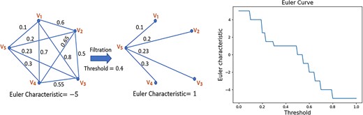
Pictorial representation of the process of constructing an EC curve of a graph: (i) filter the graph using a given threshold and compute the corresponding Euler characteristic, (ii) plot the EC for a sequence of increasing thresholds.
The EC, denoted by |$\eta $|, of a graph is defined by the difference in the number of vertices and the number of edges:
For instance, the EC of the leftmost graph in Fig. 2 is |$\eta = 5-10 = -5$|.
In order to obtain a low-dimensional descriptor for complex objects (such as graphs, images, matrices, fields, etc.), EC is often combined with a process known as filtration to generate an EC curve, which can be used to quantify the topology of the complex object. Given an edge-weighted graph |$(\mathsf{V},\mathsf{E}, \mathsf{W})$| and a threshold |$\ell $|, the filtered graph for this threshold |$\ell $|, which we denote by |$(\mathsf{V},\mathsf{E}, \mathsf{W})_{\ell }$|, is obtained by removing all the edges |$e \in \mathsf{E}$| so that |$w(e)> \ell $|. This filtration step is illustrated in Fig. 2 for |$\ell = 0.4$|. For a threshold |$\ell $|, we denote the EC of the corresponding filtered graph |$(\mathsf{V},\mathsf{E}, \mathsf{W})_{\ell }$| by |$\eta _{\ell }$|. Note that for the filtered graph of Fig 2, the EC is given by |$\eta _{0.4} = 5-4 = 1$|. The EC curve is a plot between |$\eta _{\ell }$| and |$\ell $| for a series of increasing thresholds |$\ell $|. The filtration process can be stopped once the threshold is equal to the largest weight of the original graph, at which point the filtered graph is the same as the original graph. The EC curve of the leftmost graph in Fig. 2 is the rightmost graph in that figure. It has been demonstrated in [29] that EC curves retain important characteristics of the graph and are therefore useful representations of 2D graphs using 1D vectors.
To represent a multivariate time series |$\widetilde{\mathbf{X}}_{d}^{(n,:,:)} \in \mathbb{R}^{\tilde{p}_{d} \times t_{d}}$| of subject |$n \in [1:N]$| using an EC curve, we first find the |$\tilde{p}_{d}$| by |$\tilde{p}_{d}$| precision matrix, or the |$\tilde{p}_{d}$| by |$\tilde{p}_{d}$| correlation matrix or the |$\tilde{p}_{d}$| by |$\tilde{p}_{d}$| covariance matrix from |$\widetilde{\mathbf{X}}_{d}^{(n,:,:)}$| (by treating the multiple time points in the time series as different samples of a given variable), and denote this matrix by |$M \in \mathbb{R}^{\tilde{p}_{d} \times \tilde{p}_{d}}$|. Since |$M$| is a symmetric matrix, it represents an edge-weighted graph. The matrix |$M$| is then subjected to a sequence of increasing thresholds to obtain an EC curve using the filtration process described above. The resulting EC curve is a |$1$|D representation of the time series |$\widetilde{\mathbf{X}}_{d}^{(n,:,:)}$| that can then be used as input to the integration and classification step. If the number of thresholds used during the filtration process is |$x$|, then the EC method converts |$\widetilde{\mathbf{X}}_{d} \in \mathbb{R}^{N \times \tilde{p}_{d} \times t_{d}}$| to |$\widehat{\mathbf{X}}_{d} \in \mathbb{R}^{N \times x \times 1}$|, which is low-dimensional.
Functional principal component analysis
FPCA is a dimension reduction method similar to PCA, which can be used for functional or time series data. Here, we use FPCA to convert longitudinal data |$\widetilde{\mathbf{X}}_{d} \in \mathbb{R}^{N \times \tilde{p}_{d} \times t_{d}}$| into a one-dimensional form |$\widehat{\mathbf{X}}_{d} \in \mathbb{R}^{N \times (xp_{d}) \times 1}$|, by calculating |$x$|-dimensional scores for each of the |$p_{d}$| variables, where |$x$| is the number of functional principal components considered for each variable. Specifically, for any given variable |$j$| of view |$d$|, |$\widetilde{\mathbf{X}}_{d}^{:,j,:} \in \mathbb{R}^{N \times t_{d}}$| is the collection of univariate time series of all |$N$| subjects for that variable |$j$| (where |$d \in [1:D]$| and |$j \in [1:\tilde{p}_{d}]$|). FPCA first finds the top |$x$| functional principle components (FPCs): |$f_{1}(t), f_{2}(t), \dots , f_{x}(t) \in \mathbb{R}^{1 \times t_{d}}$| of the |$N$| time series in |$\widetilde{\mathbf{X}}_{d}^{:,j,:}$|. These |$x$| FPCs represent the top |$x$| principal modes in the |$N$| univariate time series and are obtained using basis functions such as B-splines and wavelets. Each of the |$N$| univariate time series in |$\widetilde{\mathbf{X}}_{d}^{:,j,:}$| is then projected on each of the |$x$| FPCs to get an |$x$|-dimensional score for each subject |$n \in [1:N]$|, corresponding to this variable. The scores of all |$\tilde{p}_{d}$| variables are stacked together to obtain a |$\tilde{p}_{d} x$|-dimensional vector for that subject. Thus, with the FPCA method, we convert longitudinal data |$\widetilde{\mathbf{X}}_{d} \in \mathbb{R}^{N \times \tilde{p}_{d} \times t_{d}}$| to cross-sectional data |$\widehat{\mathbf{X}}_{d} \in \mathbb{R}^{N \times (x p_{d}) \times 1}$|.
In the Synthetic Analysis of EC and FPCA Section, we compare EC and FPCA using simulations. We demonstrate that when the covariance structure between the classes differs, the EC curves are particularly better at feature extraction than the functional principal components. However, EC curves are not as effective as FPCA in distinguishing between longitudinal data of different classes when the classes have a similar covariance structure and only differ in their temporal trends.
Step 3: integration and classification
In this step, we describe our approach to integrate the output data from any of the first two steps or the original input data, if the first two steps are skipped. Denote by |$\{\widehat{\mathbf{X}}_{d} \in \mathbb{R}^{N \times \hat{p}_{d} \times \hat{t}_{d}}, d \in [1:D]\}$| the data obtained after the first two steps: selection of variables and extraction of features (where both these steps are optional). Data from |$D$| views are integrated using DeepIDA combined with GRUs (that is, DeepIDA-GRU) as described in the variable selection section. As noted, in the DeepIDA-GRU network, each cross-sectional view is fed into a dense neural network, and each longitudinal view is fed into a GRU. The role of neural networks and GRUs is to nonlinearly transform each view. The output of these networks is then entered into the IDA optimization problem (Fig. 1). By minimizing the IDA objective, we learn discriminant vectors such that the projection of the non-linearly transformed data onto these vectors results in maximum association between the views and maximum separation between classes. If the feature extraction step is skipped, then each longitudinal view, |$\widehat{\mathbf{X}}_{d} \in \mathbb{R}^{N \times \hat{p}_{d} \times \hat{t}_{d}}$| with |$t_{d}>1$|, is fed into its respective GRU in the DeepIDA-GRU network. If the feature extraction step is not skipped, then each cross-sectional (|$\widetilde{\mathbf{X}}_{d} \in \mathbb{R}^{N \times \tilde{p}_{d}}$|) and longitudinal (|$\widehat{\mathbf{X}}_{d} \in \mathbb{R}^{N \times \hat{p}_{d} \times \hat{t}_{d}}$| with |$\hat{t}_{d}=1$|) view after the first step is fed into its respective dense neural network in DeepIDA-GRU. DeepIDA-GRU performs integration and classification so that the between-class separation and between-view associations are simultaneously maximized. Similarly to the DeepIDA network [13], DeepIDA-GRU also uses the nearest centroid classifier for classification. Classification performance is compared using average accuracy, precision, recall and F1 scores.
Results
Overview of the pipeline
We investigate the effectiveness of the proposed pipeline on the longitudinal (metagenomics and metabolomics) and cross-sectional (host transcriptomics) multiview data pertaining to IBD. The preprocessed host transcriptomics, metagenomics and metabolomics datasets are represented using |$3$|-dimensional real-valued tensors of sizes |$ \mathbb{R}^{90 \times 9726 \times 1}$|, |$ \mathbb{R}^{90 \times 2261 \times 10}$| and |$ \mathbb{R}^{90 \times 93 \times 10}$|, respectively, and passed as inputs in the pipeline. In the first step, the variable selection/ranking methods LMM, DGB and JPTA are used to identify key genes, microbial pathways, and metabolites that are relevant in discriminating IBD status and/or associating the views. The top |$200$| and |$50$| variables of the metagenomics and metabolomics data, respectively, are retained using each method. For host transcriptomics data, LMM and DGB are used to select the top |$1000$| statistically significant genes. Since JPTA is only applicable to longitudinal data, no variable selection is performed on the host transcriptomics data using JPTA. The resulting datasets are then passed through the feature extraction and integration/classification steps. We investigate the performance of our feature extraction and integration and classification steps by considering the following three options.
Method 1—DeepIDA-GRU with no feature extraction: In this case, there is no feature extraction. For integration and classification with DeepIDA-GRU, the cross-sectional host transcriptomics dataset is fed into a fully connected neural network (with |$3$| layers and |$200,100,20$| neurons in these three layers), while the metagenomics and metabolomics data are fed into their respective GRUs (both consisting of |$2$| layers and |$50$| dimensional hidden unit).
Method 2—DeepIDA-GRU with EC for Metagenomics and Mean for Metabolomics: In this case, the two longitudinal views are each converted into cross-sectional form. In particular, EC (with |$100$| threshold values) is used to reduce the metagenomics data to size |$\mathbb{R}^{90 \times 100 \times 1}$|. The metabolomics data is reduced to size |$\mathbb{R}^{90 \times 50 \times 1}$| by computing the mean across the time dimension. In particular, when we visualized the EC curves of the metabolomics data, we did not find any differences between the EC curves for those with and without IBD, so we simply used the mean over time. The host transcriptomics data remain unchanged. The host transcriptomics, metabolomics and metagenomics data were then each fed into a |$3$|-layered dense neural networks with structures |$[200,100,20]$|, |$[20,100,20]$| and |$[50,100,20]$|, respectively, for integration and classification with DeepIDA-GRU (which in this case is equivalent to the traditional DeepIDA network).
Method 3—DeepIDA-GRU with FPCA for both Metabolomics and Metagenomics views: In this case, FPCA (with |$x=3$| FPCs for each variable) is used to reduce the longitudinal metabolomics and metagenomics data to cross-sectional data of sizes |$ \mathbb{R}^{90 \times 150 \times 1}$| and |$\mathbb{R}^{90 \times 600 \times 1}$|, respectively. The host transcriptomics data remain unchanged. The host-transcriptomics, metabolomics and metagenomics data were each fed into a |$3$|-layered dense neural networks with structures |$[200,100,20]$|, |$[20,100,20]$| and |$[50,100,20]$|, respectively, for integration and classification using DeepIDA.
We train and test the |$9$| possible combinations of the |$3$| variable selection methods: LMM, JPTA, and DGB and the |$3$| feature extraction plus integration/classification approaches: Method 1, Method 2 and Method 3. Owing to the limited sample size, |$N$|-fold cross-validation is used to evaluate and compare the performance of these |$9$| combinations. In particular, the model is trained on |$N-1$| subjects (where |$N=90$|) and tested on the remaining |$1$| subject. This procedure is repeated |$N$| times (hence |$N$|-folds). Average accuracy, macro precision, macro recall, and macro F1 scores are the metrics used for comparison. These performance metrics are summarized in Fig. 3. The entire procedure of |$N$|-fold cross validation is repeated for three arbitrarily selected seeds: |$0,10\,000$| and |$50\,000$|. Each of the |$9$| blocks in Fig. 3 reports the performance of the best model among the three seeds. Note that since LMM and DGB leverage information about the output labels while selecting variables, both these methods only use data from the |$N-1$| subjects in the training split of each fold. In |$N=90$| folds, since there are |$90$| different train-test splits, LMM and DGB methods are repeated |$90$| times (once for each fold). Unlike LMM and DGB, JPTA does not use the output labels during variable selection, and hence it is run once on the entire dataset.
![Performance Metrics of nine different combinations of the three feature extraction options: Method 1 (no feature extraction), Method 2 (EC based feature extraction) and Method 3 (FPCA-based feature extraction); and the three variable selection methods: LMM, DGB and JPTA. In addition, the performance of MildInt $[21], [22]$ (no feature extraction and MildInt network for classification) is included in combination with the three variable selection options for comparison. For blocks of the same color, the darker shade signifies better overall accuracy.](https://oup.silverchair-cdn.com/oup/backfile/Content_public/Journal/bib/25/4/10.1093_bib_bbae339/2/m_bbae339f3.jpeg?Expires=1747902285&Signature=j2Bl31rZF4Tkeq3~0IxdGDPa1HGj7tMkg2dMHexegQjWL3Iusuj8o3daOvcHF4VBPQ8Ppu~Dv7RdV0nwryHQynHA0dGz6BvB9k8YSvT43Nx~E7xYC9Zq0jTr8yqkMGz9xd7r8Ps9ydDvkFEPG8EqA3stDSO5FKfRc-BObkvsxPUKGJddJnV6EUQ5lgxPu2DUiWd6H1-nEG~Il0Qov-~ajsXY9EntAzmVdcZSVmHvxCvEPn4KLYMLGvJ-eSukxKPZfF4eKrrb6RVWV8YAZ2z~S-7jhBUbrpXlVPcaGJ9PhwZdZIShhANj8iHMTuKnnxB9DrcQR15dkF229V-jHvAZKQ__&Key-Pair-Id=APKAIE5G5CRDK6RD3PGA)
Performance Metrics of nine different combinations of the three feature extraction options: Method 1 (no feature extraction), Method 2 (EC based feature extraction) and Method 3 (FPCA-based feature extraction); and the three variable selection methods: LMM, DGB and JPTA. In addition, the performance of MildInt |$[21], [22]$| (no feature extraction and MildInt network for classification) is included in combination with the three variable selection options for comparison. For blocks of the same color, the darker shade signifies better overall accuracy.
Classification performance of the proposed pipeline on the IBD longitudinal and cross-sectional data
Examining the rows in Fig. 3, we observe that the classification results based on the variables selected by JPTA are slightly worse than LMM and DGB. The lower performance of JPTA could be due to (i) JPTA is a purely unsupervised method and does not account for class membership in variable selection and is therefore not as effective for classification tasks as LMM or DGB; (ii) no variable selection was performed on the host transcriptomics data since JPTA is applicable only to longitudinal data. The classification results based on the variables selected by LMM and DGB are comparable with small variations that depended on the feature extraction method used before integration and classification. The classification results of the feature extraction method FPCA (Method 3) applied to the variables selected by LMM are slightly better than the feature extraction method EC (Method 2) and the direct DeepIDA-GRU application without feature extraction (Method 1). Meanwhile, the EC and FPCA feature extraction methods and DeepIDA-GRU (no feature extraction) yield comparable classification results when applied to the variables selected by DGB. Examining the columns in Fig. 3, it is evident that the three methods (Method |$1$|, Method |$2$| and Method |$3$|) have comparable results in the IBD application. The direct DeepIDA-GRU-based approach (Method 1) performs best with DGB; the EC (Method 2) and the FPCA (Method 3) approaches work best with LMM and DGB.
Moreover, to compare our proposed pipeline with existing methods, we have also included the performance of the deep learning method [20, 21] in Fig. 3. [20, 21] propose a network consisting of one-layer GRUs (one for each view), followed by a logistic regression classifier. In particular, data from each view are fed into a GRU module, and the outputs of all the GRUs are then concatenated. This concatenated output is then fed into a logistic regression classifier for classification. Our proposed pipeline differs from the aforementioned method in three important ways. First, the outputs of the three views are integrated using IDA in DeepIDA-GRU, while in the method of |$[21],[22]$|, the outputs are simply concatenated. Second, the integrated output is classified using the nearest centroid classifier in DeepIDA-GRU, while in the method of |$[21],[22]$|, the concatenated outputs are fed into a logistic regression classifier. Third, in the DeepIDA-GRU network, we use three-layer GRUs, while in the methods of [20, 21], a single-layer GRU is proposed. Due to the lack of an integration mechanism and a more simplistic one-layer architecture, the method proposed in [20, 21] does not perform as well as the DeepIDA-GRU network proposed in our paper. Since [20, 21] do not include any variable selection methods, we have used their classification framework in conjunction with the three variable selection methods (LMM, JPTA, DGB) proposed in our paper for a fair comparison. Note that we have used the code of [20, 21] for the implementation of the MildInt network.
Variables identified by LMM, JPTA and DGB
We compare and analyse the top variables selected by LMM, JPTA and DGB. As discussed earlier, both LMM and DGB are performed |$90$| times (once for each fold). Each method generates |$90$| distinct sets of selected variables. For LMM, the variables in each set are ranked according to their corresponding p-values, whereas, for DGB, the variables in each set are ranked according to their eff_prop scores (equation (1)). For LMM, an overall rank/score is associated to every variable using Fisher’s approach for combining p-values (Supplementary Material). Note that if the Fisher combined p-value is equal to zero for multiple variables, these variables will be assigned the same score. For the DGB method, the average eff_prop value is computed to combine the |$90$| scores of each variable. Lastly, JPTA is performed once, and we choose variables with nonzero coefficients.
Figure 4 shows the intersection between the sets of variables selected by LMM, DGB and JPTA for the three views. Figure 5(a)–(c) shows the top |$10$| variables selected by DGB from each view. In Fig. 5(d), we use violin plots to show the distribution of the top |$5$| host transcriptomic genes selected by DGB. The median expressions of the genes are different between the two classes. Furthermore, in Figure 5(e) and (f), we show the mean time series curves for the metagenomics and metabolomics views. In these figures, the average of the univariate time series of all the participants in the IBD and non-IBD classes is used to calculate two mean curves for the top five variables. Figure 5 is exclusive to the DGB approach. Similar analyses for the LMM and JPTA methods are provided in the Supplementary material, with corresponding figures.
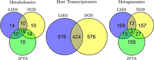
Venn diagrams showing the overlap between the top |$1000, 50$| and |$200$| variables selected from the host transcriptomics, metabolomics and metagenomics views, respectively, by the three variable selection methods LMM, DGB and JPTA (except JPTA with host transcriptomics view because JPTA does not work with cross-sectional views).
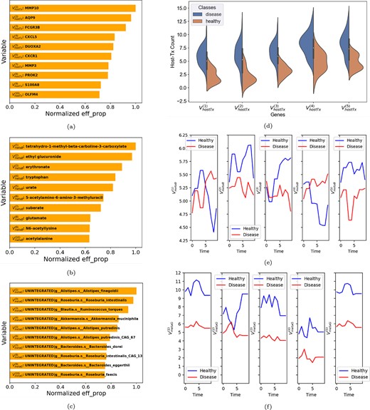
Top |$10$| variables selected by DGB from the |$\text{(a)}$| host-transcriptomics, |$\text{(b)}$| metabolomics and |$\text{(c)}$| metagenomics views, along with their combined and normalized eff|${\_ }$|prop scores. In |$\text{(d)}$|, the top |$5$| host-transcriptomics genes are statistically compared between the two classes using violin plots. In |$\text{(e)}$| and |$\text{(f)}$| respectively, the top |$5$| metabolites and metagenomic pathways are compared between the two classes using mean time series plots.
Literature analysis of top variables
There is evidence in the literature to support an association between many of the highly-ranked variables and IBD status. We first consider a few host transcriptomics genes selected by LMM or DGB. The IFITM genes have been associated with the pathogenesis of gastro-intestinal tract [30]. LIPG has been observed to have altered level in Ulcerative Colitis (UC) tissue [31]. AQP9 has been shown to have predictive value in Crohn’s disease [32]. CXCL5 has been observed to have significantly increased levels in IBD patients [33]. FCGR3B is associated with UC susceptibility [34]. The MMPs (matrix metalloproteinases) like MMP3 and MMP10 have been shown to be upregulated in IBD [35, 36]. DUOXA2 has been substantiated as an IBD risk gene [37]. The genes S100A8 and S100A9 have been linked with colitis-associated carcinogenesis [38]. LILRA3 has been observed to be increased in IBD patients [39].
We next consider some of the top metabolites selected by LMM, DGB or JPTA. Uridine has been identified as a therapeutic modulator of inflammation and has been studied in the context of providing protective effects against induced colitis in mice [40]. Suberate is one of the metabolites significantly affected by neoagarotetraose supplementation (which is a hydrolytic product of agar used to alleviate intestinal inflammation) [41]. The authors of [42] suggest saccharin to be a potential key causative factor for IBD. Docosapentaenoic Acid (DPA) has been shown to alleviate UC [43]. Decrease of pantothenic acid in the gut has been remarked as a potential symptom of IBD-related dysbiosis [44]. Valerate has been observed to be altered in UC patients [45]. It has been suggested that uracil production in bacteria could cause inflammation in the gut [46]. Thymine is a pyrimidine that binds to adenine, and adenine has been suggested as a nutraceutical for the prevention of intestinal inflammation [47]. Ethyl glucuronide is used as a biomarker to diagnose alcohol abuse [48], and alcohol consumption is common in IBD patients [49].
We next consider the metagenomics pathways selected by LMM, DGBUlcerative Colitis (UC) or JPTA. We find that the genus Alistepis [50], Roseburia [51], Blautia [52] and Akkermansia [53] have been often linked to IBD and gut health. Several unintegrated pathways involving these genus have been identified by the DGB method as significant. Butanol has been identified as statistically significant (using univariate analysis) in IBD and non-IBD groups [54], and the pathway PWY-7003 selected by LMM is associated with glycerol degradation to butanol. Thiazole has been associated with anti-inflammatory properties against induced colitis in mice and pathway PWY-6892 (selected by LMM) is associated with thiazole biosynthesis. Tryptophan has been shown to have a role in intestinal inflammation and IBD [55] and the pathway TRPSYN-PWY associated with L-tryptophan biosynthesis is one of the key pathways selected by LMM. Increased levels of L-arginine are correlated with disease severity for UC [56] and the pathway PWY-7400 associated with L-arginine biosynthesis has been selected by JPTA. Thiamine is associated with symptoms of fatigue in IBD [57] and the pathway PWY-7357 associated with thiamine formation is selected by JPTA.
As evidenced by these examples from the literature, we illustrate that many genes, metabolitesUlcerative Colitis (UC) and pathways selected by the three methods have been linked to IBD. However, there are some selected variables that may not have been directly examined in the context of IBD. For example, we could not find a direct link of the metagenomic pathways: PWY-7388 (selected in the top |$25$| by JPTA) for IBD. However, this pathway has been associated with psoriasis and it has been observed that patients with psoriasis have increased susceptibility to IBD [58]. Thus, the unstudied genes/metabolites/pathways that the three variable selection methods have discovered may potentially be novel variables linked to IBD.
Synthetic analysis of EC and FPCA
FPCA and Euler curves (EC) provide important one-dimensional representations of longitudinal data. These methods have particular significance because the extracted features can be used with a broad spectrum of existing integration methods that only allow cross-sectional views. Using synthetic simulations, we unravel key properties of EC and FPCA. These simulations demonstrate that Euler curves are better at distinguishing between classes when the covariance structure of the variables differs from one class to another. FPCA performs better when the time-trend of the variables differs between the classes. In addition to comparing EC and FPCA, we also illustrate the performance of the direct DeepIDA-GRU approach, where the feature extraction step is skipped and the longitudinal views are directly fed into DeepIDA-GRU. GRUs have the ability to distinguish certain complicated time-trend differences that pose challenges for FPCA and EC methods. However, FPCA and EC are computationally faster compared to GRUs. Moreover, as demonstrated by these simulations, training a GRU can be challenging and one needs to closely monitor problems like overfitting, diminishing gradients, hyperparameter tuning etc and their out-of-the-box performance may be even worse than the simpler methods like FPCA and EC.
To compare EC, FPCA and direct DeepIDA-GRU, we use the following three approaches on synthetically generated multiview longitudinal data: (i) DeepIDA-EC: EC is used to extract one-dimensional features from the longitudinal views and the extracted features are fed into the DeepIDA network for integration and classification; (ii) DeepIDA-FPC: FPCA is used to extract features from the longitudinal views and the extracted features are fed into the DeepIDA network for integration and classification; and (iii) DeepIDA-GRU: no one dimensional features are extracted from the longitudinal views and the data from the longitudinal views are directly fed into the DeepIDA-GRU network for integration and classification. The synthetic datasets we generate are balanced between classes and we use the classification accuracy as a metric for this comparison.
Here, we consider |$K=2$| classes, |$D=2$| views and |$N = 500$| subjects. Each view |$d$| (for |$d \in [1:2]$|) consists of |$p_{d} = 250$| variables and |$T=20$| time points. We denote by |$C_{1}$| and |$C_{2}$| the noise covariance matrices corresponding to classes |$1$| and |$2$|, respectively. These covariance matrices are constructed as follows:
where both |$C_{\text{unif}}$| and |$C_{\text{power}}$| are |$p_{1}+p_{2}$| by |$p_{1}+p_{2}$| matrices whose entries are identically and independently generated from the Uniform|$(0,1)$| and Power|$(10)$| distributions, respectively. Here, Power|$(10)$| is the power distribution (inverse of Pareto distribution) with parameter |$a=10$|, whose probability density function is given by |$f(x;a) = a x^{a-1}, x \in [0,1], {a \in (0,\infty )}$|. Moreover, |$\epsilon $| is a parameter that we manipulate to vary the amount of structural difference between |$C_{1}$| and |$C_{2}$|. In particular, when |$\epsilon =0$|, |$C_{1} = C_{2}$| and the two classes have the same covariance structure. When |$\epsilon = 1$|, the entries of |$C_{1}$| and |$C_{2}$| have completely different and uncorrelated distributions.
We let |$\phi _{d,k}$| and |$\delta _{d,k}$| be the auto-regressive (AR) and moving-average (MA) parameters, respectively, for the ARMA(1,1) process, corresponding to the |$d$|th view (|$d \in \{1,2\}$|) and the |$k$|th class (|$k \in \{1,2\}$|). For these simulations, these ARMA parameters for the two classes are chosen to be
where |$\eta $| is another parameter that is varied to control the amount of difference between the ARMA parameters of the two classes.
The synthetic longitudinal data of subject |${n \in [1:N]}$| for view |${d \in [1:2]}$| is given by a collection of |$T$| vectors: |$\mathbf{X}_{d}^{(n,:,:)}= \{\mathbf{X}_{d}^{(n,:,1)}, \mathbf{X}_{d}^{(n,:,2)}, \cdots , \mathbf{X}_{d}^{(n,:,T)}\}$| (where |${\mathbf{X}_{d}^{(n,:,t)} \in \mathbb{R}^{p_{d}}}$|). Let |$\mathbf{X}^{(n,:,t)} = \left [\mathbf{X}_{1}^{(n,:,t)}, \mathbf{X}_{2}^{(n,:,t)}\right ]^{\prime}$|, |$\mathbf{w}^{(n,t)} = \left [\mathbf{w}_{1}^{(n,t)}, \mathbf{w}_{2}^{(n,t)}\right ]^{\prime}$|, |$\boldsymbol{\phi }_{:,\kappa (n)} = \left [{\phi }_{1,\kappa (n)},{\phi }_{2,\kappa (n)}\right ]^{\prime}$| and |$\boldsymbol{\delta }_{:,\kappa (n)} = \left [{\delta }_{1,\kappa (n)},{\delta }_{2,\kappa (n)}\right ]^{\prime}$|, where |$\kappa (n)$| is the class to which the |$n$|th subject belongs and the vectors |$\mathbf{w}_{1}^{(n,t)}$| and |$\mathbf{w}_{2}^{(n,t)}$| are jointly distributed as |$\mathbf{w}^{(n,t)} \sim \mathcal{N}(\mathbf{0}, C_{\kappa (n)})$| for all |$t \in [1:T]$|. Then the multiview data |$\mathbf{X}^{(n,:,t)}$| of the subject |$n$| at time |$t$| are generated according to an ARMA|$(1,1)$| process with AR and MA parameters given by |$\boldsymbol{\phi }_{:,\kappa (n)}$| and |$\boldsymbol{\delta }_{:,\kappa (n)}$|, respectively, and the noise covariance matrix |$C_{\kappa (n)}$| as follows:
where, |$\circ $| represents the element wise product.
For any given value of |$(\eta , \epsilon )$|, a total of |$100$| longitudinal multiview datasets are generated randomly according to equation (5), where in each dataset, there are approximately |$50$| percent of the subjects in class |$1$| and class |$2$| respectively. The three approaches: DeepIDA-GRU, DeepIDA-EC and DeepIDA-FPC are used for the classification task. All the feed-forward networks consist of |$3$| layers with |$[200,100,20]$| neurons, respectively. All GRUs contain |$3$| layers with |$256$| dimensional hidden vector. The synthetic analysis is divided into two cases:
Case 1: different covariance matrices, same ARMA parameters: In this case, |$\eta = 0$| and |$\epsilon $| assumes the following set of values: |$\epsilon \in \{0.25,0.5,0.75,1\}$|. Note that a larger |$\epsilon $| means more difference in the covariance structure of the variables between the two classes and, therefore, easier for the methods to classify. Figure 6 provides a visual representation of the superiority of EC compared to FPCA for this case. In this figure, the synthetic multivariate time series data (of view |$1$|), generated with |$\epsilon = 0.75$|, for a subject of class |$1$| and a subject of class |$2$| are shown in Fig. 6(a). The EC curves of all the |$N$| subjects are shown in Fig. 6(b) (which shows that the EC curves can clearly distinguish between the two classes). The |$3$| dimensional FPC scores are plotted in Fig. 6(c) and we notice that FPCA cannot distinguish between the two classes in this case. In Fig. 8(a), we compare the performance of the three methods on |$100$| randomly generated datasets for each |$\epsilon \in \{0.25,0.5,0.75,1\}$|. In particular, we use box plots to summarize the classification accuracy achieved by the three methods on these |$100$| datasets.
Case 2: same covariance matrices, different ARMA parameters, no reverse operation: In this case, |$\epsilon = 0$| and |$\eta $| takes values in |$\eta \in \{0.25,0.5,0.75,1\}$|. Note that larger |$\eta $| corresponds to a larger difference in the ARMA parameters between the two classes and therefore easier for the methods to classify. Figure 7 shows visually that FPCA can clearly distinguish between the two classes, whereas EC cannot. In this figure, the synthetic multivariate time series data (of view |$1$|), generated with |$\eta = 0.75$|, for one subject of class |$1$| and one subject of class |$2$| are shown in Fig. 7(a). The EC curves of all the |$N$| subjects are shown in Fig. 7(b) (which shows that the EC curves are unable to distinguish between the two classes). The |$3$| dimensional FPC scores are plotted in Fig. 7(c) which shows that FPCA performs better at distinguishing between the two classes in this case. In Fig. 8(b), we compare the performance of the three methods on |$100$| randomly generated datasets for each |$\eta \in \{0.25,0.5,0.75,1\}$|. In this figure, we summarize the classification accuracy achieved by the three methods on these |$100$| datasets using box plots.
Visual comparison between EC and FPCA: Case 1—The two classes have different covariance matrices (with |$\epsilon =0.75$|), but the same ARMA parameters (that is, |$\eta = 0$|). Euler curves can distinguish between the two classes, whereas FPCA cannot.
Visual comparison between EC and FPCA: Case 2—The two classes have the same covariance matrix (that is, |$\epsilon =0$|), but different ARMA parameters (with |$\eta = 0.75$|). FPCA can distinguish between the two classes, whereas EC cannot.
Box plots are used to compare the accuracy of the three methods: DeepIDA-GRU, DeepIDA-FPC and DeepIDA-EC in two cases. In Case 1, the covariance structure between the two classes differs, the difference being proportional to the magnitude of |$\epsilon \in \{0.25,0.5,0.75,1\}$|, but the ARMA parameters are the same (i.e. |$\eta = 0$|). In Case 2, the ARMA parameters between the two classes differ, with the difference being proportional to the magnitude of |$\eta \in \{0.25,0.5,0.75,1\}$|, but the covariance structure is the same (i.e. |$\epsilon = 0$|). The box plots illustrate the spread of accuracies attained by the three methods for |$100$| distinct synthetically generated datasets, for each pair of |$(\epsilon ,\eta )$| values.
The box plots in Figure 8(a) and 8(b) show that DeepIDA-EC performs better at classifying subjects when the covariance structure of the two classes is different, whereas DeepIDA-FPC performs better when the ARMA parameters of the two classes differ. DeepIDA-GRU does not outperform either of these methods even though it has the potential to handle much more complex tasks. This could be mainly due to the fact that the DeepIDA-GRU network was not fine-tuned for each of the randomly generated datasets, which could have led to overfitting/underfitting on many of these datasets.
Discussion
Data collected from multiple sources is increasingly being generated in many biomedical research. These data types could be cross-sectional, longitudinal data, or both. However, the literature for integrating both cross-sectional and longitudinal data is scarce. This work began to fill in the gaps in the existing literature. Motivated by and used for the analysis of data from the IBD study of the iHMP, we have proposed a deep learning pipeline for (i) integrating both cross-sectional and longitudinal data from multiple sources while simultaneously discriminating between disease status; and (ii) identifying key molecular signatures contributing to the association among views and separation between classes within a view. Our pipeline combines the strengths of statistical methods, such as the ability to make inference, reduce dimension, and extract longitudinal trends, with the flexibility of deep learning, and consists of variable selection/ranking, feature extraction, and joint integration and classification. For variable selection/ranking, methods applicable to one view at a time (i.e. LMMs), two longitudinal views (i.e. JPTA), and multiple cross-sectional and longitudinal views (i.e. DGB) were considered. For feature extraction, we considered the FPCA and EC curves. For integration and classification, we implemented Deep IDA with gated recurrent units [DeepIDA-GRU].
When we applied the pipeline to the motivating data, we observed that for variable selection, LMM and DGB achieved slightly better performance metrics than JPTA probably because they are supervised methods– information on class labels is used in variable selection– and they are applicable to more than two views. For feature extraction, the performance of both EC and FPCA was comparable, and both methods performed similarly to the direct DeepIDA-GRU approach without feature extraction. Our research revealed multi-omics signatures and microbial pathways that differentiate between individuals with and without IBD, some of which have been documented in previous studies, while others are associated with diseases linked to IBD, offering potential candidates for exploration in IBD pathobiology. We also compared the performance of EC and FPCA using synthetic datasets and found that these methods outperformed each other in different scenarios. EC performed better when the covariance structure of the variables was different between the two classes, while FPCA outperformed EC when there was a difference in the time trends between the two classes.
Deep learning is typically used with a large sample size to ensure generalizability. The main limitation of this work is the small sample size (|$n=90$| subjects) of the IBD data, which motivated our work but we attempted to mitigate against potential overfitting/underfitting issues through the use of variable selection, feature extraction and leave-one-out-cross-validation instead of |$n$|-fold cross-validation (which would have significantly reduced the sample size for training). Variable selection is widely regarded as an effective technique for high-dimensional low sample size data and helps avoid overfitting and high-variance gradients [59, 60]. In this work, we explored both linear methods for variable selection (LMM and JPTA) and non-linear deep learning-based methods (DGB). More analysis is needed to determine whether the DGB bootstrapping procedure scales well with increasing data sizes. Future work could consider validating the proposed methodology on multiview data with larger sample sizes. Additionally, for larger and more complicated data, it may be worthwhile to investigate whether integrating other deep learning networks like transformers and 1D convolutional networks in the DeepIDA pipeline would yield better results for handling longitudinal data than the DeepIDA with GRUs implemented in this work.
Despite the above limitations, we believe that our pipeline for integrating longitudinal and cross-sectional data from multiple sources that combines statistical and machine learning methods fills an important gap in the literature for data integration and will enable biologically meaningful findings. Our extensive investigation of the scenarios under which FPCA outperforms EC curves and vice versa sheds light on the specific scenarios for using these methods. Furthermore, our application of real data has resulted in the identification of molecules and microbial pathways, some of which are implicated in the literature and thus providing evidence to corroborate previous findings, while others are potentially novel and could be explored for their role in the pathobiology of IBD.
We propose a deep learning pipeline capable of seamlessly integrating heterogeneous data from multiple sources and effectively discriminating between multiple classes.
Our pipeline merges statistical methods with deep learning, incorporating variable selection and feature extraction techniques such as functional principal component analysis (FPCA) and Euler characteristic curves (EC). It also includes integrative discriminant analysis using dense feed-forward and recurrent neural networks for joint integration and classification.
We examined when FPCA is more effective than EC curves and vice versa. FPCA yields better classification when longitudinal trends differ between classes; EC yields better classification under unequal class covariance.
Adding variable selection to deep learning led to a strong classification performance, even with a small sample size.
The IBD data application shows the potential application of our pipeline to identify molecular signatures that discriminate disease status over time.
Conflict of Interest: The authors declare that there is no conflicts of interest.
Funding
The project described was supported by the Award Number 1R35GM142695 of the National Institute of General Medical Sciences of the National Institutes of Health. The content is solely the responsibility of the authors and does not represent the official views of the National Institutes of Health.
Data availability
The Python code for implementing DeepIDA-GRU is publicly available on GitHub at https://github.com/lasandrall/DeepIDA-GRU.
References
