


Abstract
Identifying the causal relationship between genotype and phenotype is essential to expanding our understanding of the gene regulatory network spanning the molecular level to perceptible traits. A pleiotropic gene can act as a central hub in the network, influencing multiple outcomes. Identifying such a gene involves testing under a composite null hypothesis where the gene is associated with, at most, one trait. Traditional methods such as meta-analyses of top-hit |$P$|-values and sequential testing of multiple traits have been proposed, but these methods fail to consider the background of genome-wide signals. Since Huang’s composite test produces uniformly distributed |$P$|-values for genome-wide variants under the composite null, we propose a gene-level pleiotropy test that entails combining the aforementioned method with the aggregated Cauchy association test. A polygenic trait involves multiple genes with different functions to co-regulate mechanisms. We show that polygenicity should be considered when identifying pleiotropic genes; otherwise, the associations polygenic traits initiate will give rise to false positives. In this study, we constructed gene–trait functional modules using the results of the proposed pleiotropy tests. Our analysis suite was implemented as an R package PGCtest. We demonstrated the proposed method with an application study of the Taiwan Biobank database and identified functional modules comprising specific genes and their co-regulated traits.
Introduction
Exploring the genotype–phenotype relationship has historical roots in Mendel’s observations of Pisum, based on which he proposed the concept of “pleiotropy”, suggesting that multiple traits are controlled by a single factor. The term “gene” emerged alongside pleiotropy, though its molecular definition was unclear. Various hypotheses arose, including Beadle’s “one-gene/one-trait” hypothesis and Gruneberg’s distinctions of genuine and spurious pleiotropy; he used “genuine pleiotropy” to describe a gene of two distinct primary products and “spurious pleiotropy” to describe a gene of a single primary product that initiates different pathways [1, 2]. The consensus on gene–trait mechanisms emerged with Beadle’s “one-gene/one-enzyme” hypothesis. Over time, the term pleiotropy evolved with the emergence of modern molecular biology insights that categorized pleiotropy based on the origin of cross-phenotype associations. As illustrated in Fig. 1, “biological pleiotropy” involves a single variant or more variants in the same gene regulating multiple traits; “mediated pleiotropy” reflects a genetic variant that influences one trait, which affects another; and “spurious pleiotropy” may result from a study design artifact, confounder bias, or strong linkage disequilibrium [3].
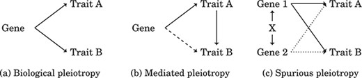
Types of pleiotropy. (a) Biological pleiotropy indicates that a gene regulates multiple traits; therefore, the gene is responsible for the association of the traits. (b) Mediated pleiotropy refers to when a gene regulates Trait B while fully or partially mediated by Trait A. Testing whether an indirect effect exists can distinguish (b) from (a). (c) Unmeasured confounding between genes may initiate a spurious pleiotropic gene (Gene 2) due to a biological pleiotropic gene (Gene 1). The solid line indicates authentic causation, the dashed line indicates potential authentic causation, and the dotted line indicates spurious causation.
Characterizing biological pleiotropy amidst diverse cross-phenotype associations poses a major challenge that has prompted the development of various approaches. These methods fall into two main categories: ‘multivariate tests’ that facilitate simultaneous analysis of multiple traits and ‘univariate tests’ that initially focus on one trait and then integrate the results across traits [3–5]. Multivariate tests rely on traditional regression models such as linear mixed models [6], generalized estimating equations [7, 8], and multivariate generalized linear models [9] and necessitate individual-level data to consider inter-trait covariance [4, 5]. The core idea is jointly assessing the target gene’s associations with all traits before conducting sequential tests to identify gene–trait pairs of effects. Univariate tests employ integrated approaches including traditional ‘meta-analyses’ that combine summary statistics and ‘pleiotropy-informed’ methods that consider trait correlations. Meta-analyses involve Fisher’s method, which entails directly combining |$P$|-values [10], utilizing fixed/random effects models that combine effect estimates and standard errors [11–13], performing CPMA while presuming at least two associated traits [14], and adopting the MultiMeta/MTAG approach with inverse variance-weighted meta-analyses [15, 16]. Pleiotropy-informed methods consider the conditional false discovery rate (FDR) given the association of both phenotypes [17, 18], and MetaSAT [19] and PLEIO [20] employ a variance component test statistic that accounts for pleiotropy.
Although numerous approaches exist, only a handful incorporate the components of the composite null into their testing. The null hypothesis of “no pleiotropic effect” involves two scenarios: (i) The genetic factor does not regulate any trait and (ii) the genetic factor only regulates one trait. When testing a gene with two specific traits, the true null distribution becomes a mixture of three simple nulls with unknown proportions: the gene regulates none of the target traits, the gene only regulates the first trait, and the gene only regulates the second trait. Conventional methods often overlook the proportions of the simple nulls in the composite null, necessitating additional techniques for result adjustment. For instance, MTAG [16] only considers the first scenario as null and later adjusts the FDR using a different formula. MetaSAT [19] selects a minimum |$P$|-value by tuning a pleiotropy-level parameter, and PLEIO [20] employs importance sampling to obtain accurate |$P$|-values. Under the composite null distribution, Huang [21] proposed a composite test that generates uniformly distributed |$P$|-values while considering the proportions of the three simple nulls, and PLACO [22] was the first to apply the composite test for detecting pleiotropic variants.
In this paper, we present a pleiotropy-informed univariate approach that utilizes the composite test to identify pleiotropic genes while accounting for traits’ polygenic nature. Polygenic traits introduce challenges in identifying pleiotropic genes due to the role of unknown co-regulating genes as unmeasured confounders; disregarding polygenicity can lead to serious false positives. The remainder of the paper is organized as follows: first, we introduce the pleiotropic gene model and employ the aggregated Cauchy association test (ACAT) [23] to assess gene–trait associations. Second, we introduce a gene-level pleiotropic test based on the composite test Huang [21] proposed. Third, we address the complexities arising from polygenic traits and detail how we mitigated this issue through the “gene-adjusting step.” Fourth, we conduct comprehensive simulations to assess the sensitivity and FDR at different pleiotropic and polygenic levels. Finally, we demonstrate the proposed pleiotropic test using the Taiwan Biobank dataset. Recent research on pleiotropy using the UK Biobank [24] has shown that 81.2% of genes exhibit pleiotropy when assessing multiple traits, a finding that underscores the importance of recognizing pleiotropy as a primary focus in gene–trait association investigations. Consequently, we integrated significant gene–trait associations into co-regulation modules and further annotated these modules to understand their functions in the gene regulatory network.
Materials and methods
Pleiotropic gene model
We define the pleiotropic problem by introducing the following notations: For each individual, let |$S$| be the variant, |$Y$| be the phenotypic trait, and |$\textbf{X}$| be the covariates with the first element of 1 for the intercept. Consider a genome-wide experiment |${\mathcal{E}}$| that includes |$g$| genes and a given trait |$Y$| to be evaluated, denoted as |$\mathcal{E}=\big \{{{\mathbb{G}}^{i}}\big |i\in 1,\ldots ,g\big \}$|. For |$i\in \{1,\ldots ,g\}$|, the |$i$|th gene–trait relationship can be described by the following general linear model:
where |$f(\cdot )$| is a link function, |$\textbf{S}^{i}=\big (S^{\mathit{ij}}\big )$|, |$\boldsymbol \beta ^{ {i}}=\big (\beta ^{\mathit{ij}}\big )$|, |$j\in \{1,\ldots ,s_{i}\}$|, and |$s_{i}$| indicates the number of variants for the |$i$|th gene. The |$i$|th gene is a pleiotropic gene of traits |$Y_{a}$| and |$Y_{b}$| if we reject the null hypothesis for |${{\mathbb{G}}^{i}}$| as follows:
where |$\boldsymbol \beta ^{\mathit{i}}_{a}=\big (\beta _{a}^{\mathit{ij}}\big )$| and |$\boldsymbol \beta ^{\mathit{i}}_{b}=\big (\beta _{b}^{\mathit{ij}}\big )$| are coefficients for |$Y_{a}$| and |$Y_{b}$| in Equation (1). The test statistics assessing the gene–trait associations, namely |$T_{a}^{i}$| and |$T_{b}^{i}$|, are constructed with the correlated estimators |$\hat{\boldsymbol \beta }^{\mathit{i}}_{a}$| and |$\hat{\boldsymbol \beta }^{\mathit{i}}_{b}$| and their covariance matrices if needed. Thus, |$T_{a}^{i}$| indicates the strength of the paths |$\textbf{S}^{i}\rightarrow Y_{a}$|, |$T_{b}^{i}$| indicates the strength of the paths |$\textbf{S}^{i}\rightarrow Y_{b}$|, and their product represents the pleiotropic effect of the |$i$|th gene. For simplicity, we drop the superscript |$i$|. We employed the ACAT [23] to construct |$T_{a}$| and |$T_{b}$| because it can combine correlated estimators while disregarding the correlation between them when computing |$P$|-values. Let |$\textbf{Z}_{a}$| and |$\textbf{Z}_{b}$| be the statistics that scale the variance of |$\hat{\boldsymbol \beta }_{a}$| and |$\hat{\boldsymbol \beta }_{b}$| to 1; we can then obtain |$T_{a}=T_{\text{ACAT}}(\textbf{Z}_{a})$| and |$T_{b}=T_{\text{ACAT}}(\textbf{Z}_{b})$| from
where the component |$\tan \big [\big \{2\Phi \big (\big |Z^{j}\big |-3/2\big )\big \}\pi \big ]$| follows a standard Cauchy distribution under the null, and |$w_{j}$|s are arbitrary weights that can be incorporated as prior knowledge.
To apply the composite test Huang [21] proposed, we transform each |$T_{a}$| into |$a$| and |$T_{b}$| into |$b$| using the following equation:
where |$p_{\alpha }$| is the two-sided |$P$|-value of |$T_{a}$|, |$p_{\beta }$| is the two-sided |$P$|-value of |$T_{b}$|, and sign|$(\hat{\boldsymbol \theta })=\big \{1-2\text{I}\big (\sum _{j=1}^{s_{i}}\hat{\theta }^{j}<0\big )\big \}$| is a function for determining the collective direction of the regression coefficients (i.e. sign|$(\hat{\boldsymbol \theta })=1$| if the summation of the direction is positive; otherwise, sign|$(\hat{\boldsymbol \theta })=-1$|), |$\text{I}(\cdot )$| denotes an indicator function, and |$\Phi (\cdot )$| denotes the cumulative distribution function of a standard normal distribution. To fulfill the assumption the composite test requires, we proved that |$a$| and |$b$| converge to a standard normal distribution under the null; the proof can be found in the Supplementary Material. Then, for |$i\in \big \{1,\ldots ,g\big \}$|, the |$P$|-value of the pleiotropic effect for the |$i$|th gene towards |$Y_{a}$| and |$Y_{b}$| can be calculated using the following equation:
where |$F(z)$| can be calculated through the numerical integration of the probability density function of the normal product distribution, and |$\epsilon $| is bounded and can be ignored (see [21] for details). The variances of |$a$| and |$b$| can be estimated using a collection of hypothesis tests for a similar purpose, e.g. a series of tests in a genome-wide analysis. Thus, the |$P$|-values derived from the composite test can be understood as an approximation of the composite null distribution based on data-driven proportions. Please refer to Fig. 2 for a detailed illustration and the algorithm.
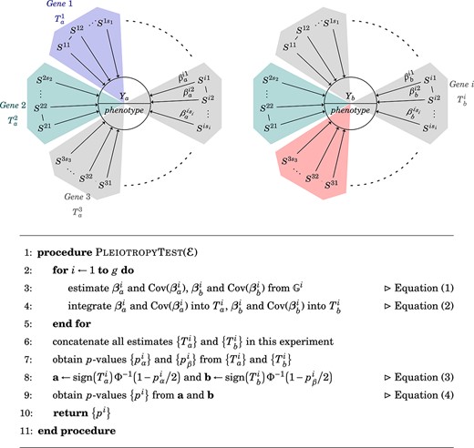
Identification of pleiotropic genes. The identification of pleiotropic genes entailed two main steps: (a) Construct two multivariate statistics of |${{\mathbb{G}}^{i}}$| for |$Y_{a}$| and |$Y_{b}$|, and (b) assess the pleiotropic effect using the composite test as described in Equation (4). We evaluated each geneÑtrait relationship by testing the null hypothesis in Equation (1). A colorful background indicates a successfully detected effect, and gray indicates no effect. In this demonstrated case, Genes 1 and 2 influence Trait |$Y_{a}$|, and Genes 2 and 3 influence Trait |$Y_{b}$|; thus, Gene 2 is pleiotropic.
Polygenic trait model
In the previous section, we employed ACAT to assess gene–trait associations and combined it with the composite test to investigate the pleiotropic effect. However, the independence assumptions required in Equation (4) may be violated when the traits are polygenic. Supplementary Figure S3 shows that co-regulating genes are confounders between |$Y_{a}$| and |$Y_{b}$|; therefore, ignoring the polygenicity is a compromise associated with unmeasured confounding.
To manage the confounding effects of co-regulating genes, we recommend applying the “gene-adjusting step” before the main analysis if individual-level data are available; the idea is to adjust for other genes with strong signals toward the target trait. If we assume no unmeasured confounding, then applying the gene-adjusting step is sufficient to achieve |$a^{u}\perp \mkern -9.5mu\perp a^{v}$| and |$a^{u}\perp \mkern -9.5mu\perp b^{u}$|. Here, we use |$a\perp \mkern -9.5mu\perp b$| to indicate that |$a$| is independent from |$b$|. If individual-level data are unavailable, we recommend applying the decorrelation step suggested by PLACO [22]; the idea here is to test the pleiotropic effect for two specific linear combinations of |$Y_{a}$| and |$Y_{b}$| that meet the independence assumptions. If we assume no unmeasured confounding, then applying the decorrelation step at least ensures |$a^{u}\perp \mkern -9.5mu\perp b^{u}$|. Note that if we apply the decorrelation step, we can only conclude that the target gene has a pleiotropic effect toward |$Y_{a}$| and |$Y_{b}$| as a module since we actually test a pleiotropic effect toward the linear combination of the two traits. Please refer to the Supplementary Material for additional details regarding our practical management approach.
After conducting a phenome-wide analysis, we can construct the gene–trait co-regulation modules by combining pleiotropic genes with their co-regulating traits as shown in Fig. 3. Further analysis, such as identifying mediated pleiotropy or network annotation, can be conducted.
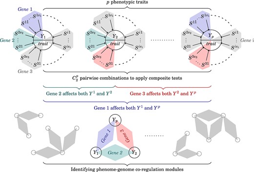
Identifying gene–trait co-regulation modules. To analyze data at the phenome-wide level, we identify pleiotropic genes from pairwise trait combinations. Next, we collect the pleiotropic genes with corresponding traits and construct the co-regulation modules for further network analyses.
Results and discussion
Simulation
To mimic practical situations, we simulated phenome-wide analysis in which the traits were polygenic and the data were collected from the same population. One experiment simulation included five traits and 10 000 genes of 500 individuals. For the |$i$|th gene, we randomly generated a vector of 20 correlated variants |$\textbf{S}^{i}$| using a multivariate normal distribution with a mean of 1 and the correlation coefficient |$\rho $|. The correlation coefficient between variants was either 0 or 0.3, following Sun and Lin [25], to ensure a positive definite matrix. We discretized the vector’s value using the mean as a cut-off to generate binary variants. We then generated two covariates |$\textbf{X}$| using Normal|$(0,1)$| and the phenotypic trait |$P$| according to the following equation,
where |$\mathbb{C}$| is the set of genes that potentially contribute toward the trait, |$\boldsymbol \beta _{\mathit{X}}=1$|, and |$\epsilon $| also follows Normal|$(0,1)$|. For each |$i\in \mathbb{C}$|, if the |$i$|th gene has no signal, |$\boldsymbol \beta ^{\mathit{i}}=0$|; otherwise, we assign |$h$| variants non-zero signals following Normal|$(\mu ,v)$| and assign the remaining |$(20-h)$| variants coefficients of zero. We modified |$h$| to demonstrate the effects of signal sparsity at the gene level, applied |$|\mathbb{C}|$| for the polygenic level at the trait level, and considered the percentage of shared genes between the two traits, i.e. |$|\mathbb{C}_{a}\cap \mathbb{C}_{b}|$|, as well as the strength of the pleiotropy effects, where the size of the set is represented by |$|\cdot |$|. The modified criteria are presented in Supplementary Table S1.
For gene–trait associations, we compared the ACAT with two state-of-the-art multivariate statistics to detect genome-wide signals, namely the generalized Berk–Jones statistic (GBJ) [25] and generalized higher criticism (GHC) [26]. For pleiotropy assessment, we compared the composite test with two classical tests, namely “the joint significance test” [27] and “the normality-based test” [28], as well as with two state-of-the-art pleiotropy-informed tests, namely “the conjunctional FDR” [17] and “PLEIO” [20] (for the settings, see the Supplementary Results).
Performance of the composite test under the null
We have shown that our |$P$|-value calculations were sufficiently accurate for controlling the genome-wide type I error rate. We examined two types of null scenarios: “the complete null setting,” which indicated that all genes were |$H_{0\emptyset }$| in a genome-wide experiment as depicted in Fig. 4a, and “the single-trait null setting,” which indicated that most genes were |$H_{0\emptyset }$|, but some genes were |$H_{0\alpha }$| or |$H_{0\beta }$| in a genome-wide experiment as depicted in Fig. 4b. Using the composite test with the gene-adjusting step, we controlled the average type I error rates up to the significance level |$\alpha =10^{-5}$| in complete and single-trait nulls as shown in Supplementary Table S2. Note that the polygenic traits induced dependency between |$a^{v}$| and |$a^{u}$| and between |$a^{v}$| and |$b^{v}$| as shown in Supplementary Fig. S3.
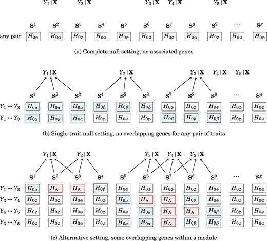
Polygenic traits. (a) All genes in the complete null setting showed no association with any traits. (b) Some genes in the single-trait null setting were associated with only one trait (single-trait null), and others had no association with any traits (complete null). For example, considering |$Y_{1}\leftrightarrow Y_{2}$|, the genes associated with |$Y_{1}$| (|$\textbf{S}^{1}, \textbf{S}^{2}, \textbf{S}^{3}$|) did not overlap with the genes associated with |$Y_{2}$| (|$\textbf{S}^{4}, \textbf{S}^{5}, \textbf{S}^{6}$|), so |$\textbf{S}^{1}, \textbf{S}^{2}, \textbf{S}^{3}, \textbf{S}^{4}, \textbf{S}^{5}, \textbf{S}^{6}$| should be identified as a single-trait null, whereas the other genes that did not share any association with |$Y_{1}$| and |$Y_{2}$| should be identified as a complete null. (c) Some genes in the alternative setting were associated with two traits (alternative), some genes were associated with one trait (single-trait null), and others were not associated with any traits (complete null). For example, considering |$Y_{1}\leftrightarrow Y_{2}$|, |$\textbf{S}^{2}$| and |$\textbf{S}^{3}$| regulate both traits, so they should be identified as alternative; |$\textbf{S}^{1}$| and |$\textbf{S}^{4}$| regulate |$Y_{1}$| and |$Y_{2}$|, respectively, so they should be identified as a single-trait null; other genes showed no shared associations with |$Y_{1}$| and |$Y_{2}$| and should be identified as a complete null.
Performance of the composite test under the alternative
We evaluated the composite test’s performance using the “alternative setting” described in Fig. 4c in which some genes were |$H_{\text{A}}$|, |$H_{0\alpha }$|, or |$H_{0\beta }$|, but most genes were still |$H_{0\emptyset }$| in a genome-wide experiment. Figure 5 shows the average sensitivity and FDR of the five pleiotropic tests (the composite test, the conjunctional FDR, the joint significance test, the normality-based test, and PLEIO), with different pleiotropic levels (i.e. the percentage of gene overlap between two traits, 30%/80%/100%) and with different polygenic levels (i.e. the number of associated genes per trait, 20/30/40 genes) as described in Supplementary Table S1. Figure 5a shows that across all levels of pleiotropy, the composite test exhibited the highest sensitivity compared with the other four tests. Additionally, the composite test achieved the theoretical FDR most closely at a pleiotropic level of 100%. Figure 5b shows that when the polygenic level was higher (|$>30$| genes per trait), PLEIO had the best sensitivity, but we also found that PLEIO had the highest FDR among all the tests. After PLEIO, the composite test had the best sensitivity across all levels of polygenicity.
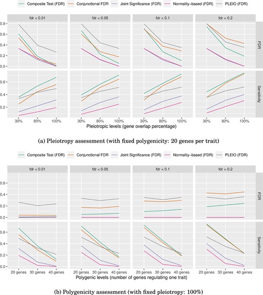
Evaluation at different pleiotropic and polygenic levels. We used several significance cut-offs to evaluate the sensitivity and FDR for the five pleiotropy tests. The findings are as follows: (a) across all pleiotropic levels, the composite test had the highest power. When the pleiotropic level reached 100%, only the composite test achieved the theoretical FDR. (b) When the polygenic level was higher (40 genes per trait), PLEIO had the best sensitivity but also had a higher FDR. After PLEIO, the composite test had the best power. When the polygenic level was the highest (40 genes per trait), the normality-based test did not identify any significant genes with respect to any of the significance cut-offs.
For the above results of the five pleiotropic tests, we applied the gene-adjusting step in advance to fairly compare the powers and FDRs. Supplementary Figure S4 shows the composite test’s total significance proportion, power, and FDR with and without applying the gene-adjusting step. If individual-level data are unavailable, we cannot apply the gene-adjusting step (so we may apply the decorrelation step to weaken the confounding effect from other co-regulating genes); we should therefore be aware that the high significance proportion may be attributed to false positives. Supplementary Figure S4 also shows the total significance proportion, power, and FDR for the three gene–trait association statistics. As shown in Supplementary Fig. S4 and Table S2, we found that the ACAT had the lowest FDR and the highest power. Additionally, it offers extremely fast computation since there is no underlying matrix computation.
Taiwan biobank analyses
We applied the proposed testing pleiotropy detection procedure to data obtained from the Taiwan Biobank [29, 30]. After the preprocessing step (refer to the Supplementary Materials for specific details on quality control and exclusion criteria, which largely followed the approach described in [31]), we obtained data from 58 449 individuals with SNP information that could be integrated into 17 833 genes. Additionally, we considered 26 biochemical analysis results as traits and included covariates such as sex, age, smoking status, alcohol consumption, betel nut consumption, the top 10 principal components of the full SNP matrix, and variants of the top 20 associated genes as covariates. We applied the composite test, the joint significance test, the normality-based test, the conjunctional FDR, and PLEIO on all pairs of 26 biochemical analyses (325 trait pairs). For each pair, we adjusted the nominal |$P$|-values of the pleiotropic genes using the FDR with a significance cut-off of 0.1.
To identify significant trait pairs, we checked whether the number of significant genes using nominal |$P$|-values (|$\alpha =0.05$|) exceeded the number of expected genes under the null. We found that the composite test identified 58 of 325 trait pairs, PLEIO identified 12 pairs, the conjunctional FDR did not provide nominal |$P$|-values, and the other two methods failed to identify any significant trait pairs. Next, for each significant trait pair, we identified significant pleiotropic genes using the FDR cut-off. In summary, the composite test identified 1525 pleiotropic genes, the joint significance test identified 361 genes, the normality-based test identified 153 genes, the conjunctional FDR identified 1762 genes, and PLEIO identified 783 genes from among the 66 significant trait pairs (union of the composite test and PLEIO).
Figure 6a is a Venn diagram [32] of the pleiotropic genes the five pleiotropic tests identified. The genes the joint significance and normality-based tests identified were all included among the genes the composite test or the conjunctional FDR identified, which shows that the two classical methods may have lower power, but their results were still in accordance with the composite test and the conjunctional FDR. However, PLEIO did not identify the 277 genes the classical methods identified. Note that we did not apply the gene-adjusting step for PLEIO in the real application to facilitate comparison of all the methods’ original analytical procedures. We also found that the composite test and the conjunctional FDR shared consistent results as both methods identified 1242 genes. The conjunctional FDR identified more significant genes than the composite test, which may be attributed to polygenicity-induced false positives as shown in Fig. 5b or to the manual setting of the primary significance cut-off. The results for the top 10 trait pairs are listed in Fig. 6b; the complete results for the 66 significant trait pairs can be found in Supplementary Table S2. We found that the composite test and the conjunctional FDR shared similar results; they both provided hundreds of pleiotropic genes for the top pairs, and their top pairs were identical. As for the other three methods, the joint significance and normality-based tests had conspicuously lower power; PLEIO identified fewer genes among the top 10 pairs but more genes among the remaining pairs.
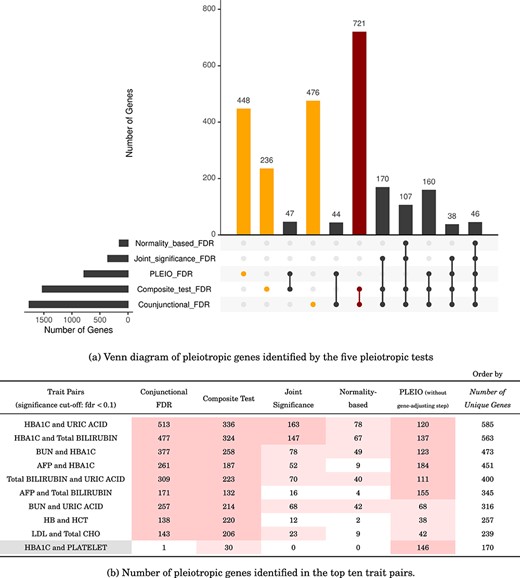
Pleiotropic genes identified by the five pleiotropic tests. (a) Orange bars mark the genes identified by a single test; the dark red bar indicates the largest overlap, showing that the conjunctional FDR and the composite test produced consistent results. (b) Gray cells indicate the pairs identified by PLEIO. Regarding the cell color of the numbers of the significant genes, dark pink indicates the pairs with over 100 genes, and light pink indicates the pairs with over 20 genes.
We analyzed the biological functions of the pleiotropic genes identified by the composite test. We used the number of genes as edge weights (at least 20 genes) to perform a clustering analysis of the 58 significant trait pairs, and we obtained four co-regulating trait modules as illustrated in Fig. 7. The upper module (brown) included the traits of diabetes and renal functions regulated by 742 pleiotropic genes. The pathway analyses showed enrichment in several metabolic pathways, especially a secondary metabolic pathway, glucuronidation [33, 34], which was enriched in four databases. The top genes included ADAMTS20, a metalloprotease that targets glycosylated proteins [35, 36], and MUC21, a gene that encodes a large membrane-bound glycoprotein [37, 38]. The right module (purple) included conventional indicators of liver damage regulated by 175 pleiotropic genes. The top genes included ZNRD1-AS1, a long non-coding RNA associated with an increased risk of hepatocellular carcinoma (HCC) [39], promotes malignant lung cell proliferation [40], and influences cervical cancer development [41], and TTN-AS1, another long non-coding RNA that promotes HCC progression [42–44].
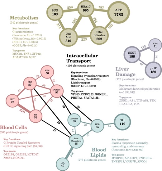
Four trait modules co-regulated by pleiotropic genes. We identified four modules: the right one (purple) is related to liver damage, the lower one (teal) is related to blood lipids, the left one (red) is related to blood cells, and the upper one (brown) is related to metabolism. Colored edges indicate genes within a module, and black edges indicate genes between modules. We also annotated the nodes with the number of trait-associated genes and annotated the edges with the number of pleiotropic genes. The significance cut-off was set as an FDR below 0.1.
The lower module (teal) included the traits of blood lipids regulated by 273 pleiotropic genes; the enriched pathways conspicuously showed the dynamic functions of lipoprotein regulation. The left module (red) included the traits of blood cells and proteins regulated by 306 pleiotropic genes. The top genes included OR51B4 and OR52E2, both of which belong to G-protein-coupled receptors (GPCR), as well as KCTD17, which is a key regulator of cAMP signaling [45–47]. We also identified 110 pleiotropic genes in the four edges linking the red and teal modules. Pathway analyses showed that these genes were related to “intracellular transport.” The top genes included GGNBP1, which leads to mitochondrial fragmentation [48], and VPS35, which generates a vesicle for delivering mitochondrial fragments to lysosome [49, 50]. In summary, the proposed method provided preliminary screening to identify pleiotropic genes and their co-regulating traits; however, careful examination is still required to further understand these genes’ roles in regulating multiple outcomes.
Conclusion
In this study, we integrated ACAT with the composite test to identify pleiotropic genes that may influence polygenic traits. By comparing the results of five pleiotropic tests, we observed that the composite test exhibited superior sensitivity across all pleiotropy levels. Moreover, the composite test maintained the expected FDR in scenarios with low polygenic effects in contrast to the other tests that showed either lower or higher FDRs. We also examined the impact of incorporating a gene-adjusting step to control for genetic associations during pleiotropic gene identification. Applying our approach to the Taiwan Biobank dataset revealed four co-regulating modules with distinct biological functions and pathways, which provided valuable insights into the underlying mechanism.
Identifying pleiotropic genes with consideration of polygenic traits.
Using the composite test that meticulously manages the composite null behind the pleiotropic definition.
Analyzing Taiwan Biobank dataset and illustrating the trait modules co-regulated by the pleiotropic genes we identified.
Conflict of interest
The Authors declare no Competing Financial or Non-Financial Interests.
Funding
We thank the Ministry of Science and Technology, Taiwan (108-2118-M-001-013-MY5) and Academia Sinica (AS-CDA-108-M03) for providing funding for this study.
Data availability
The R package PGCtest is available at https://github.com/roqe/PGCtest.
References
