


Abstract
The interaction between T-cell receptors (TCRs) and peptides (epitopes) presented by major histocompatibility complex molecules (MHC) is fundamental to the immune response. Accurate prediction of TCR–epitope interactions is crucial for advancing the understanding of various diseases and their prevention and treatment. Existing methods primarily rely on sequence-based approaches, overlooking the inherent topology structure of TCR–epitope interaction networks. In this study, we present |$GTE$|, a novel heterogeneous Graph neural network model based on inductive learning to capture the topological structure between TCRs and Epitopes. Furthermore, we address the challenge of constructing negative samples within the graph by proposing a dynamic edge update strategy, enhancing model learning with the nonbinding TCR–epitope pairs. Additionally, to overcome data imbalance, we adapt the Deep AUC Maximization strategy to the graph domain. Extensive experiments are conducted on four public datasets to demonstrate the superiority of exploring underlying topological structures in predicting TCR–epitope interactions, illustrating the benefits of delving into complex molecular networks. The implementation code and data are available at https://github.com/uta-smile/GTE.
Introduction
The interaction between T-cell receptors (TCRs) and peptides (epitopes) presented by major histocompatibility complex molecules (MHC) forms the foundation of T-cell immunity [1, 2]. The interaction between TCRs and epitopes aids in the activation of T cells, enabling them to effectively combat pathogens within the body, such as bacteria, viruses, or tumor cells [3, 4]. Therefore, the precise recognition of TCRs with epitopes significantly contributes to the understanding and technological advancements in preventing and treating various diseases. However, due to the inherent complexity of this recognition mechanism, experimental detection and validation of TCR–epitope interactions are often time-consuming and costly [5]. To address these challenges, numerous computational methods have been developed to simulate TCR–epitope interactions [6–11].
TCR and epitope sequences are inherently short, making it challenging to collect a sufficient amount of Multiple Sequence Alignment (MSA) data. Consequently, it becomes difficult to effectively harness MSA-based protein models [12–14], especially when directly utilizing single sequence-based protein language models [15]. Mainstream methods typically involve sequence information for TCRs and epitopes to construct sequence-level classification models through transfer learning [8, 16–18]. Specifically, TCR and epitope sequence data are gathered from databases such as VDJdb [19], IEDB [20], and McPAS-TCR [21]. These sequences are then input into pre-trained models to obtain high-quality embeddings for TCRs and epitopes, which are subsequently used in deep learning models to predict whether TCRs and epitopes will bind.
While previous methods have obtained success, they still face three challenges in TCR–epitope prediction. (i) The interaction between TCRs and epitopes is not an isolated event but part of a complex and extensive interaction network. Networks formed by protein interactions are crucial as they depict the cellular framework and signal pathways while also influencing signal transmission within cells [22, 23]. Therefore, it draws our attention to the need for effectively utilizing the topological structure between TCRs and epitopes. However, how to efficiently exploit such topological structures to predict TCR–epitope interactions remains unexplored. The major challenge is that unlike protein–protein interactions (PPIs), where all nodes are treated as the same in a simple homogeneous graph [24], TCRs and epitopes shall be considered as two distinct types of nodes due to their biological nature. Therefore, constructing a topological structure graph for TCRs and epitopes is even more complex. (ii) TCR and epitope interaction datasets typically contain both positive and negative samples. Effectively utilizing negative sample data helps the model better understand and differentiate between positive and negative samples [25]. Current approaches often require the preparation of fixed negative sample data before training [8, 16, 17, 26], which may exceed physical memory limitations or result in high time complexity during the training process. Therefore, how to design a strategy for learning negative samples effectively is another crucial challenge. (iii) TCR–epitope prediction often encounters a severe data imbalance issue since the number of positive instances is normally much lower than the number of negatives. This imbalance could cause the model to lean toward predicting the majority class, presenting another challenge that needs to be addressed.
In order to tackle the above challenges, we propose GTE, a graph learning framework for the prediction of TCR–epitope binding specificity. To the best of our knowledge, GTE is the first attempt to capture the topological structure of the TCR–epitope interaction graph for enhancing the prediction performance. Specifically, we introduce a heterogeneous graph neural network (GNN) model based on inductive learning to form TCR–epitope binding prediction tasks as edge classification problems. Through graph learning, our model offers a more comprehensive insight into the natural environment’s topological structure of TCRs and epitopes, effectively revealing previously unseen interactions. Furthermore, we propose a novel dynamic graph learning method that allows the model to encounter a more diverse set of negative samples during the training process, without being constrained by physical memory limitations. Nevertheless, the efficient negative sampling method could potentially exacerbate data imbalance. We then employ the AUC Maximization [27] to effectively address the challenge of data imbalance.
We have conducted experiments on four public datasets under various settings to evaluate the performance of TCR–epitope interaction prediction tasks, and achieved significant improvement over the current state-of-the-art (SOTA) methods consistently. The overall contributions of our proposed GTE are summarized as follows:
Our proposed GTE is the first method to explore the topological structure to enhance TCR–epitope binding prediction tasks by introducing an inductive heterogeneous GNN.
An advanced dynamic graph learning mechanism is developed to adaptively sample negative data during training, allowing efficient learning of negative samples without being constrained by physical memory limitations.
AUC maximization is adapted in the graph domain to ensure the model maintains a more balanced and robust predictive capability, thereby overcoming the data imbalance problem.
Related work
Predicting the binding of any given TCR–epitope pair benefits many advances in healthcare, such as aiding diagnostics, vaccine development, and cancer therapies [1, 28]. Researchers have been developing models for predicting peptide immunogenicity for decades. However, compared with the theoretical diversity of TCRs, the available data are still limited, posing challenges for the development of computational prediction methods [7, 28–30].
Prior research has indicated that the CDR3 |$\beta $| sequences likely play a more significant role in determining TCR binding specificity to epitopes [31, 32]. Therefore, most sequence-based methods primarily rely on the CDR3 |$\beta $| sequence. For instance, TEIM [17] combines sequence and residue contact prediction, utilizing a two-phase training approach. TEINet [16] employs transfer learning, transforming TCR and epitope sequences into numerical vectors using separate pre-trained encoders, and uses a fully connected neural network to predict their binding specificity. pMTnet [8, 33] is a significant model for TCR–pMHC binding prediction, utilizing TCR, epitope, and MHC sequence data, setting it apart from the previous two models.
However, current methods primarily focus on learning sample similarities, often neglecting the intrinsic molecular network formed by natural interactions and overlooking the utilization of graph topological structure. In contrast, our proposed model explores a novel direction to uncover the underlying topological relationship within TCRs and epitopes, yielding superior outcomes. Furthermore, we employ a dynamic graph learning mechanism and AUC maximization strategy to efficiently sample negative data and address data imbalance issues.
Methods
The overall framework of GTE is illustrated in Fig. 1, which demonstrates that TCR–epitope binding prediction tasks are transformed into edge classification problems. Specifically, we take TCR–epitope pair data as the input to build a heterogeneous graph. TCRs and epitopes are considered nodes with different types, and the edge is established for each TCR–epitope pair. Next, we employ a GNN model on the constructed graph to predict the edge class. During the training process, we propose a novel dynamic edge update approach that adaptively samples more negative pairs, thereby allowing the model to learn from a more diverse set. Additionally, an innovative AUC loss function is designed to handle the potential data imbalance issue during the training. Detailed descriptions of each core component are presented in the following subsections.
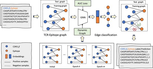
GTE framework: the training and testing datasets are labeled with two classes: positive (binding) or negative samples; the blue nodes represent TCRs (CDR3.|$\beta $|), and the orange nodes represent epitopes; the solid edges are established when TCRs and epitopes are binding, and the dashed edges represent negative samples; during the training process, we employ a GNN with two layers of GraphSAGE and a dynamic graph, along with AUC maximization; ultimately, we concatenate the node features of TCRs and epitopes, and use a Multi-Layer Perceptron to generate binding scores, which represent the probability of edges; the details of the inference phase can be found in Appendix F.
Constructing graph-based topology for TCR-Epitope
The network of direct physical interactions between proteins plays a pivotal role in facilitating information transfer among proteins [22–24, 34]. However, prior methods have predominantly concentrated on learning sample embeddings and distances, neglecting the inherent wealth of topology information.
In this study, we introduce the graph-based topological structures into TCR–epitope binding prediction. As shown in Fig. 1, we first create a heterogeneous graph, which can be represented as |$G = (V, E, X)$|, where |$V$| is the set of nodes, including TCR nodes and epitope nodes. |$E$| is the set of edges representing relationships between TCR and epitope nodes, the number of edges is equal to the total number of positive and negative TCR–epitope pairs. We use only one type of edge to represent both positive and negative samples when building the graph. The goal is to classify the established edges, where label 0 represents negative and label 1 represents positive (binding). |$X$| is the feature matrix of nodes, where each node |$v_{i}$| corresponds to a feature vector |$x_{i}$| obtained by inputting the respective sequence into the pre-trained model TCRpeg [35], i.e. |$x_{i} = \mathrm{TCRpeg}(v_{i})$|. In the constructed graph, an edge |$e_{ij}$| represents the connection between node |$v_{i}$| and node |$v_{j}$|. The label |$y_{ij}$| on |$e_{ij}$| is either 1 or 0, which indicates whether there is a connection established. Therefore, we can represent the edge set |$E$| and label set |$Y$| as follows:
The process of signal propagation entails utilizing SAGEConv [36] and a fully connected network to compute the probability output for nodes. For each node |$v_{i}$|, the signal propagation is computed using the SAGEConv layer:
where |$\mathrm{SAGEConv}^{(k)}$| represents the |$k$|-th layer of SAGEConv operation, and |$h_{i}^{(k)}$| is the representation of node |$v_{i}$| at the |$k$|-th layer, and |$\mathrm{neighbors}(v_{i})$| represents the set of neighboring nodes of node |$v_{i}$|. The features of TCR node |$v_{i}$| and epitope node |$v_{j}$| are concatenated as follows: |$h_{\mathrm{concat}}=\left [h_{i}, h_{j}\right ]$|. These concatenated features are then passed through a fully connected network represented by |$\mathrm{FC}$|, followed by a sigmoid activation function to yield the prediction probability |$p_{i j}$|:
For the loss function, we employ the BCE loss, which is commonly used for binary classification problems:
where |$N$| is the number of edges, |$y_{ij}$| is the true label (0 or 1) of the |$i$|-th edge, and |$p_{ij}$| is the predicted probability of the |$i$|-th edge being a positive (binding) event. Thus, the binding probability between TCR and epitope can be obtained while using the BCE loss function for training.
Our method constructs a heterogeneous TCR–epitope graph to leverage the topological structure, which captures correlations between sample pairs and maps the relationships between different TCRs and epitopes. At the same time, our model employs inductive learning to improve its ability to predict interactions between unknown TCRs and epitopes.
Dynamic edge updating strategy
During the graph construction process, how to establish edges for negative samples within the graph presents another challenge. We propose to use dynamic graph learning to provide the model with as many negative samples as possible at a minimal cost. At the beginning of training, negative sample edges are introduced into the initial positive-only training graph. Then, negative samples are re-sampled based on the prediction results of each iteration during the training stage. For instance, incorrectly predicted negative samples are retained, and from those correctly predicted, a proportion (|$M\%$|) is selected for re-sampling.
For the |$M\%$| of samples that require re-sampling, the same strategy is applied as used for the initial negative sample collection. For each epitope, a random selection of |$N$| (defaulting to 10) TCRs is made to create new negative samples. It is also important to ensure that these randomly generated new negative samples do not conflict with positive samples. If |$N$| negative samples cannot be found within this |$M\%$|, then as many of the remaining negative samples as possible are utilized. To ensure that the knowledge from negative samples is thoroughly learned after each dynamic negative sampling, the model is evaluated following every operation. If it surpasses the previous best result, then dynamic negative sampling is performed again in the next epoch. As shown in Fig. 1 dynamic graph module, updates with light-colored edges represent dynamic negative samples. Under the same conditions, adopting a dynamic edge updating strategy allows the model to encounter a more diverse set of negative samples at minimal cost, thus improving the efficiency of model training.
Deep AUC maximization
In the field of TCR-epitope binding prediction, the quantity of positive samples is often limited. To expand the model to learn from a larger dataset, it is common practice to use a greater number of negative samples [26]. This leads to the issue of data imbalance, which can be exacerbated by the practice of dynamic edge updating strategies. Area under the ROC Curve (AUC) is conventionally used as the evaluation metric in our tasks since it evaluates the model’s ability to rank positive samples higher than negative samples. Given this situation, a loss function designed specifically for optimizing AUC is not only better suited to address the challenges of imbalanced data but also significantly enhances model performance [27].
Specifically, consider the input space |$X \in \mathbb{R}^{\mathrm{d}}$|, and the output space |$Y\!\!=\!\!\{-1,+1\}$|. The training data follow the unknown distribution |$\rho $|, independently and identically distributed in |$Z=X \times Y$|. The ROC curve is the plot of the True Positive Rate against the False Positive Rate. For any scoring function |$f\!\!:\!\! X \rightarrow R$|, its AUC equals the probability that a positive sample ranks higher than a negative one. It is defined as follows: |$\operatorname{AUC}(f)=\operatorname{Pr}\left (f(x) \geq f\left (x^{\prime }\right ) \mid y=+1, y^{\prime }=-1\right )$|, where |$f(x)$| and |$f(x^{\prime })$| are the decision function scores. |$x$| denotes the positive samples and |$x^{\prime }$| denotes the negative samples. |$y=+1$| and |$y^{\prime }=-1$| represent its corresponding labels. The goal is to find the optimal decision function |$f$| that satisfies
The function |$\mathbb{I}(\cdot )$| takes the value 1 if the argument is true and 0 otherwise. Since |$\mathbb{I}(\cdot )$| is not continuous, it is often replaced with a convex function. In this work, we use |$ \ell _{2} \operatorname{loss}\left (1-\left (f(x)-f\left (x^{\prime }\right )\right )\right )^{2} $| as the convex function, where |$f(x)=w^{T} x$|, |$w$| denotes the parameters of the deep neural network to be learned. Overall, the maximization of AUC can be formalized as
This can be reformulated as an equivalent stochastic saddle point problem [37] with any |$w \in \mathbb{R}^{\mathrm{d}}, a, b, \alpha \in \mathbb{R}$| and |$z=(x, y) \in Z$|, where |$a$| and |$b$| can be interpreted as the mean prediction score on positive data and negative data. |$\alpha $| is a hyperparameter that controls the trade-off. Let |$p$| denote |$\operatorname{Pr}(y=1)$|, which is the the probability of a sample being in the positive class. Finally, we define a function |$F: \mathbb{R}^{\mathrm{d}} \times \mathbb{R}^{3} \times Z \rightarrow \mathbb{R}$|, AUC loss (|$L_{AUC}$|) as follows:
The final loss function is defined as follows, where |$\beta $| is a hyperparameter used to control the weights.
Overall, our proposed GTE redefines TCR–epitope binding prediction as an edge prediction task by exploring the topological structure. Moreover, an advanced dynamic graph learning mechanism is proposed to sample negative data adaptively, and AUC maximization is employed to achieve a more balanced and robust prediction in response to data imbalance issues.
Pretrained encoder
Due to the limited data on TCRs and epitopes, accurately representing TCRs or epitopes is challenging. Transfer learning has been widely used to generate embeddings for TCRs or epitopes [8, 16, 17] since it is capable of reducing the dependency on vast amounts of target domain data for constructing target learners [38–41]. In our study, we employ two types of pre-trained models to generate embeddings for TCRs and epitopes. One is based on general protein sequences as training data, while the other relies on specific TCR sequences or epitope sequences as training data. Specifically, the ESM2 [15] advanced protein pre-trained model based on the deep learning Transformer architecture aims to learn the evolutionary relationships and structural-functional features of proteins by analyzing large-scale protein sequence data, with a feature size of 1280. On the other hand, the TCRpeg [16, 35] trained on |$10^{6}$| TCR sequences or 362 456 unique epitope sequences is a probabilistic model using a deep autoregressive model architecture with gated recurrent unit layers, capturing key features of sequence inputs through unsupervised learning, with a feature dimension of 768.
Using protein language models or TCR-epitope models to generate embeddings demonstrates the flexibility of the GTE method. It highlights that the graph-based topological structure is not limited to a single type of embedding, proving its broad applicability. In subsequent experiments, unless specifically noted, TCRpeg will be used by default.
Experiments
In this section, we briefly introduce the dataset and splitting method. Details of the experimental settings are provided in Appendix A. Extensive experiments demonstrate that methods based on graph topological structure outperform all SOTA models in the field.
Experimental setup
Training and testing set splitting
In TCR-epitope studies, it is common to use five-fold cross-validation to evaluate the model’s performance[8, 16, 17]. In our study, we refer to this approach of randomly splitting data as “RandomTCR.” However, we notice that RandomTCR carries the risk of potential data leakage. Specifically, random splitting may result in overlapping TCRs between the training and validation sets. This overlap can lead to unreliable results, as the model may have already been exposed to TCRs from the validation set during training.
To mitigate this issue that exists in current studies, we first introduce the “StrictTCR” splitting approach to ensure a rigorous experimental setting. With this approach, data are divided into five folds based on unique TCRs, guaranteeing the absence of duplicate TCRs in both the training and validation sets. Furthermore, when negative samples are generated within each fold, the possibility of having identical negatives in the training and validation sets is eliminated. Therefore, StrictTCR is more scientifically rigorous as it can assess the model’s ability to handle previously unseen TCR data.
Datasets
We follow the experimental settings of SOTA TCR–epitope prediction methods [8, 16, 17], and conduct experiments on four publicly available datasets to demonstrate the effectiveness of our method.
VDJdb Dataset [19]: The VDJdb dataset consists of a curated set of 89 847 pairs of CDR3 sequences, which include both the |$\alpha $| and |$\beta $| chains of TCRs, covering three different species: humans, monkeys, and mice. We perform a series of filtering steps, retaining only entries for MHC class I and keeping only the |$\beta $| chain. Additionally, we constrain the length of CDR3 to be between 5 and 30 amino acids and the epitope length to be between 7 and 15 amino acids, and we include only human data. After all these filtering steps, the dataset is reduced to 38 533 unique CDR3|$\beta $|-epitope pairs, with 36 033 TCRs assigned to 1002 epitopes.
McPAS-TCR Dataset [21]: It is a manually curated catalog of TCR sequences, comprising 40 033 pairs of sequences, covering two species: mice and humans. We apply a similar filtering process to McPAS-TCR as we performed for VDJdb. In the end, we obtain 5102 unique CDR3|$\beta $|-epit1ope pairs, with 4975 TCRs assigned to 244 different epitopes.
TEINet Dataset [16]: TEINet is a dataset provided by the baseline. It includes 44 682 pairs of TCRs and epitopes, with 41 610 TCRs associated with 180 epitopes. TEINet provides a five-fold partition using the RandomTCR method; thus, we directly use their pre-processed data as the RandomTCR dataset. We re-sample the original data provided by TEINet to form the StrictTCR setting.
pMTnet Dataset [8]: pMTnet relies on quality metrics provided by certain databases and uses them to filter records [7, 19, 21, 31, 42–46], retaining only high-confidence pairs. For example, in VDJdb and TCRGP [7] data, they include only records with vdj.scores greater than zero. This enhances the confidence in specific TCR–epitope interactions. This process ultimately yields 31 203 pairs of TCRs and epitopes, with 28 604 TCRs associated with 426 epitopes.
Negative data
In the field of machine learning, especially in classification problems, negative samples are essential. They help the algorithm learn what features not to associate with a positive class, hence enabling more accurate and generalized model performance. This distinction is crucial for effectively training a model to differentiate between various classes [47, 48]. However, the publicly available TCR–epitope interaction datasets often only include positive samples, which presents a challenge for training and evaluating models. Therefore, we adopt a commonly used method for generating negative samples [8, 16, 17, 26]. Within each set, negative examples are generated by mismatching the positive data, i.e. combining an epitope sequence with a TCR different from its cognate target. To more comprehensively evaluate our model, we generate 1x, 5x, and 10x negative samples for each dataset, with 10x being the default setting.
Experimental results
Performance of GTE
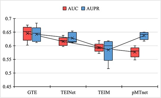
We compare the performance of three baseline methods, TEINet [16], TEIM [17], and pMTnet [8], employing StrictTCR data splitting approaches. These methods are evaluated using two key metrics, AUC and Area under the Precision-Recall Curve (AUPR), with results averaged from five-fold cross-validation. Furthermore, to ensure a fair comparison with the baselines, the results for “RandomTCR,” as well as the five-fold and standard deviation outcomes, are presented in Appendix B.
Figure 2 shows the results for four datasets using the StrictTCR split method. Our results are significantly better than the baselines. It is noteworthy that the AUC score of the baseline model TEINet is 0.607 under StrictTCR, slightly lower than their reported score of 0.610|$\pm $|0.002 under RandomTCR. This difference may be due to StrictTCR’s elimination of potential data redundancy, which could make training more challenging and thus reduce TEINet’s performance. However, our GTE method achieves an AUC of 0.863 on the TEINet dataset. This firmly attests to the advantage of utilizing the topological structures of the graph when predicting TCR–epitope interactions. Moreover, the baseline TEINet also reports an AUC of 0.603|$\pm $|0.004 using the pMTnet method on their dataset, and similarly, we obtain an AUC of 0.616 for pMTnet under the TEINet dataset. The decrease in pMTnet’s performance compared with pMTnet-reported results is due to the omission of MHC information. The reason for excluding MHC information is to maintain consistency and ensure a fair comparison, as it is not included in any of the other experiments. Since the baseline methods treat each TCR–epitope pair as an independent input, and fail to consider the correlations among different types of TCR and epitope, their performances slightly decrease under the StrictTCR data splitting approach. Unlike baseline methods, our method constructs a heterogeneous graph of TCR–epitope interactions, which not only exploits the correlations between sample pairs but also explores the relationships between different TCRs and epitopes. Inductive representation learning has been shown to efficiently produce high-quality embeddings for previously unobserved data using node feature information [36], and enhances our model’s ability to explore interactions between previously unseen TCRs and epitopes. Therefore, our method is also competitive under the StrictTCR splitting approach, further illustrating the benefits of graph-based topological methods.
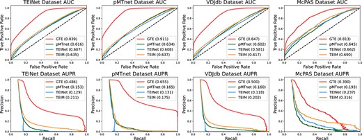
Comparison results under StrictTCR setting; experiments are conducted on four datasets using three baseline models; the first row demonstrates the visualizations of AUC scores and the second row illustrates the AUPR scores.
Furthermore, the application of our GTE method to the pMTnet dataset yields an impressive AUC of 0.910. This score not only greatly surpasses the baseline but also stands out as the highest score among all four datasets. This result might be attributed not only to our successful leverage of the topological structure of the graph but also potentially due to the pMTnet dataset combining data from various sources, carefully curated to retain only high-confidence data [7, 19, 21, 31, 42–46], while the other datasets may contain some lower confidence data. However, even in the other three datasets with potentially noisy data, our results still surpassed all baselines. This suggests that the baseline methods might face challenges when adapting to diverse sources of data, and they exhibit particular sensitivity when dealing with low-confidence data. In contrast, our method is capable of capturing the variations between different datasets, and it demonstrates robust performance even when faced with low-confidence data. This confirms the superiority of our graph-based topological structure method.
Moreover, we conduct a thorough analysis of the model complexity, as illustrated in Table 1. The results demonstrate the efficiency of graph-based topological methods in maintaining high prediction accuracy while conserving computational resources.
Single sequence protein model evaluation
Inspired by recent advancements in single-sequence protein language models [15], we explore the suitability of large-scale protein language models to generate the embeddings for TCRs and epitopes. We select ESM2 [15] as a comparative baseline. ESM2 is a SOTA protein language model that is extensively trained and optimized, demonstrating outstanding performance in various protein-related tasks, including structural prediction and functional annotation. In our study, we utilize two different variants of ESM2, with 650M and 3B parameters, respectively. On the other hand, we employ TCRpeg [35] model provided by TEINet [16]. TCRpeg is an autoencoder model that utilizes recurrent neural networks with GRU layers to capture the features of TCRs and epitopes. TCRpeg is trained on a dataset comprising |$10^{6}$| TCR sequences and 362 456 unique epitopes, resulting in pre-trained models for epitopes and TCRs.
The performance of these three different embedding representations is evaluated in our GTE method and a comparative analysis is conducted on four datasets. To ensure a fair comparison, we keep the model parameters and data consistent, only changing the sequence embeddings. The results and conclusions of our study are as follows. Table 2 displays the results for the same four datasets under the StrictTCR split. Each result represents the average of five-fold cross-validation. Appendix C displays the RandomTCR split results.
Comparison experiments are conducted to evaluate different input embeddings using the proposed GTE model on four datasets with the StrictTCR setting; both AUC and AUPR scores are reported; each result derives from five-fold cross-validation and includes standard deviations; the best scores are marked in bold
| Embeddings | TEINet Dataset | pMTnet Dataset | VDJdb Dataset | McPAS Dataset | ||||
|---|---|---|---|---|---|---|---|---|
| AUC | AUPR | AUC | AUPR | AUC | AUPR | AUC | AUPR | |
| ESM2(650M) | 0.824 |$\pm $| 0.008 | 0.459 |$\pm $| 0.017 | 0.899 |$\pm $| 0.003 | 0.632 |$\pm $| 0.008 | 0.829 |$\pm $| 0.005 | 0.466 |$\pm $| 0.009 | 0.742 |$\pm $| 0.023 | 0.305 |$\pm $| 0.032 |
| ESM2(3B) | 0.814 |$\pm $| 0.015 | 0.441 |$\pm $| 0.029 | 0.897 |$\pm $| 0.003 | 0.625 |$\pm $| 0.007 | 0.827 |$\pm $| 0.005 | 0.462 |$\pm $| 0.009 | 0.746 |$\pm $| 0.019 | 0.308 |$\pm $| 0.030 |
| TCRpeg | 0.839|$\pm $| 0.005 | 0.486|$\pm $| 0.012 | 0.911|$\pm $| 0.003 | 0.655|$\pm $| 0.007 | 0.847|$\pm $| 0.005 | 0.500|$\pm $| 0.010 | 0.813|$\pm $| 0.014 | 0.390|$\pm $| 0.031 |
It can be observed that using pre-trained models based on TCR and epitope sequences yields slightly better results than those generated by large-scale protein language models. One possible reason could be the relatively shorter nature of TCR and epitope sequences, which could lead to a loss in performance when using embeddings generated by large protein language models. However, this also prompts us to consider whether using large-scale epitope language models or large-scale TCR-epitope models could yield even better results. Furthermore, the results also underscore the effectiveness of our graph-based topology and its strong generalization. Whether based on protein language models or TCR-epitope language models, our approach consistently outperforms the current SOTA results.
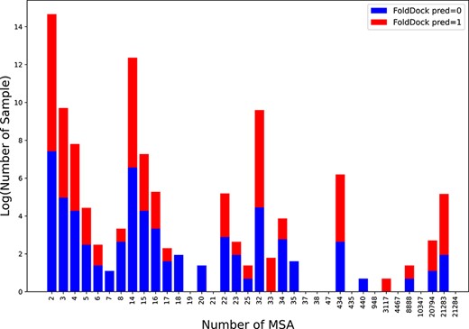
Illustration of prediction results for positive samples from the McPAS dataset using the FoldDock predictor; the x-axis represents the number of MSAs, and the y-axis represents the log-transformed sample counts; the red color signifies correct predictions, and the blue color indicates incorrect predictions.
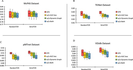
Ablation experiments are conducted on four datasets; the y-axis represents AUC scores, and the x-axis shows two partitioning methods; in the figures, the crosses (X) represent the average AUC scores obtained from five-fold cross-validation, while the lines indicate the median; Panel A displays results for the McPAS Dataset, Panel B for the TEINet Dataset, Panel C for the pMTnet Dataset, and Panel D for the VDJdb Dataset.
MSA-based protein model evaluation
Recently, significant progress has been made with large-scale protein models based on MSA in the field of protein prediction [13, 14, 49]. FoldDock [12] aims to enhance PPI predictions using AlphaFold2 [14]. Inspired by FoldDock, we assessed the feasibility and limitations of applying AlphaFold2 to simulate human TCR–epitope interactions. Specifically, we input all the positive samples of TCR and epitope sequences to FoldDock predictor. The process continues with MSA searches and evaluations, culminating in the quantification of interface contacts. Due to the extensive time required for MSA extraction and the demanding GPU resource requirements of the complex AlphaFold2 model structure, we only report the performance on the smallest McPAS dataset in Fig. 3. We input all the positive samples (binding) from McPAS into the baseline FoldDock and calculate the accuracy based on the predicted interface contacts. Since we consider the short lengths of the TCR and epitope sequences, defining a prediction as correct based on just one interface contact represents a relaxation of the baseline, yielding an accuracy of 0.4292. Under more stringent constraints, such as defining predictions with more than two interface contacts as correct, the result is 0.3701. When predictions with more than three interface contacts are considered correct, the result is 0.3267 (flip classes for 0.6733). In contrast, our method achieves an accuracy of 0.7740. More details can be found in Appendix D, with the MSA count and prediction results for all positive samples reported. Such results indicate a challenge when applying MSA-based protein language models directly to TCR–epitope predictions. The limitation may be due to the naturally shorter lengths of TCRs and epitopes, making it difficult to find a substantial number of MSAs. Figure 3 presents a statistical analysis of the impact of the number of MSAs on the results. To enhance clarity, we take the logarithm of the sample counts, with the y-axis representing the log-transformed sample counts and the x-axis showing the number of MSAs. The red color indicates correct predictions, while the blue color signifies incorrect predictions. A trend is evident, with a slight improvement in accuracy as the number of MSAs increases (larger red fraction). This supports our assertion that the direct application of MSA-based protein language models to TCR–epitope interactions is challenging due to the limited availability of MSAs for TCRs and epitopes. On the other hand, it reaffirms the superiority of our graph-based topological approach.
Ablation study
In this section, we present the results of our ablation experiments using box plot, as depicted in Fig. 4. We extend our experimental findings for the four datasets: TEINet, pMTnet, VDJdb, and McPAS. Here, “|$GTE$|” denotes the use of dynamic graph training along with the inclusion of AUC loss. “|$w/o Both$|” signifies the absence of AUC loss and dynamic graph strategy.
The results indicate that each component of the proposed method consistently enhances predictive performance. Even in the absence of AUC loss and dynamic graph strategies, our model still outperforms all baseline methods on the AUC scores, also with a smaller standard deviation compared with other conditions. This suggests that the graph-based topological approach is inherently robust and efficient. Incorporating dynamic graph learning and AUC maximization leads to a significant improvement in model performance, which proves that dynamic graph learning promotes the acquisition of a more diverse set of negative samples, and AUC maximization effectively addresses the challenge of data imbalance.
Different negative sample settings
To verify the robustness of our model under different negative sample settings, Tables 3 and 4 report the results under the positive-to-negative sample ratios of 1:1 and 1:5, respectively. Specifically, we keep the parameters and structure of the model unchanged, only replacing the training and testing datasets. The results clearly demonstrate that our model consistently achieves the best results, regardless of the negative sample setting. With the positive-to-negative sample ratios of 1:1 to 1:5, the AUPR for all methods decreases as the number of negative samples increases, which may be due to an increase in false positives. Furthermore, the AUC for all methods increases as the number of negative samples increases, which might be attributed to the larger training set enabling better learning about negative samples, resulting in lower scores for these samples during prediction and thus promoting further training of the model. This also supports our point that richer information can be learned from a large number of negative samples, which can effectively improve the model.
Comparison of model performance with a 1:1 positive-to-negative sample ratio; results are obtained from five-fold cross-validation; AUC and AUPR scores, along with their standard deviations, are reported; the best scores are highlighted in bold
| Models | TEINet Dataset | pMTnet Dataset | VDJdb Dataset | McPAS Dataset | ||||
|---|---|---|---|---|---|---|---|---|
| AUC | AUPR | AUC | AUPR | AUC | AUPR | AUC | AUPR | |
| TEINet | 0.608 |$\pm $| 0.008 | 0.615 |$\pm $| 0.008 | 0.619 |$\pm $| 0.005 | 0.612 |$\pm $| 0.006 | 0.588 |$\pm $| 0.005 | 0.597 |$\pm $| 0.004 | 0.687 |$\pm $| 0.021 | 0.697 |$\pm $| 0.021 |
| TEIM | 0.606 |$\pm $| 0.004 | 0.617 |$\pm $| 0.004 | 0.618 |$\pm $| 0.004 | 0.617 |$\pm $| 0.002 | 0.590 |$\pm $| 0.003 | 0.602 |$\pm $| 0.005 | 0.641 |$\pm $| 0.024 | 0.659 |$\pm $| 0.026 |
| pMTnet | 0.578 |$\pm $| 0.004 | 0.577 |$\pm $| 0.005 | 0.579 |$\pm $| 0.027 | 0.583 |$\pm $| 0.030 | 0.571 |$\pm $| 0.003 | 0.574 |$\pm $| 0.003 | 0.562 |$\pm $| 0.007 | 0.562 |$\pm $| 0.008 |
| GTE(Ours) | 0.734|$\pm $| 0.003 | 0.781|$\pm $| 0.003 | 0.813|$\pm $| 0.002 | 0.839|$\pm $| 0.003 | 0.775|$\pm $| 0.004 | 0.811|$\pm $| 0.004 | 0.743|$\pm $| 0.012 | 0.788|$\pm $| 0.017 |
Comparison of model performance with a 1:5 positive-to-negative sample ratio; results are obtained from five-fold cross-validation; AUC and AUPR scores, along with their standard deviations, are reported; the best scores are highlighted in bold
| Models | TEINet Dataset | pMTnet Dataset | VDJdb Dataset | McPAS Dataset | ||||
|---|---|---|---|---|---|---|---|---|
| AUC | AUPR | AUC | AUPR | AUC | AUPR | AUC | AUPR | |
| TEINet | 0.614 |$\pm $| 0.006 | 0.267 |$\pm $| 0.016 | 0.621 |$\pm $| 0.002 | 0.243 |$\pm $| 0.014 | 0.588 |$\pm $| 0.004 | 0.251 |$\pm $| 0.007 | 0.691 |$\pm $| 0.017 | 0.372 |$\pm $| 0.026 |
| TEIM | 0.616 |$\pm $| 0.004 | 0.285 |$\pm $| 0.008 | 0.622 |$\pm $| 0.003 | 0.263 |$\pm $| 0.003 | 0.599 |$\pm $| 0.005 | 0.273 |$\pm $| 0.005 | 0.647 |$\pm $| 0.016 | 0.354 |$\pm $| 0.022 |
| pMTnet | 0.608 |$\pm $| 0.006 | 0.262 |$\pm $| 0.005 | 0.580 |$\pm $| 0.006 | 0.218 |$\pm $| 0.005 | 0.592 |$\pm $| 0.002 | 0.251 |$\pm $| 0.004 | 0.623 |$\pm $| 0.009 | 0.281 |$\pm $| 0.015 |
| GTE(Ours) | 0.760|$\pm $| 0.008 | 0.419|$\pm $| 0.009 | 0.855|$\pm $| 0.005 | 0.598|$\pm $| 0.008 | 0.786|$\pm $| 0.002 | 0.447|$\pm $| 0.005 | 0.753|$\pm $| 0.014 | 0.392|$\pm $| 0.019 |
However, as the ratio changes from 1:5 to 1:10 (see Fig. 2), the baseline methods show varying performance in AUC across four datasets. This may indicate that baseline methods are unable to effectively handle severe data imbalances. In contrast, the AUC scores of our method continue to increase, which convincingly demonstrates that maximizing AUC can effectively address data imbalance. Moreover, employing a dynamic edge update strategy allows the model to learn more comprehensive information from more negative samples, thus enhancing model performance.
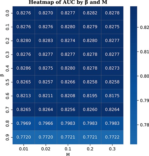
Parameter sensitivity analysis on the McPAS dataset; |$\beta $| represents the weight for AUC loss, while |$1-\beta $| is the weight for BCE loss; |$M$| controls the sampling probability for dynamic edge updates; the color varies based on the AUC scores; the darker color indicates higher AUC value.
Parameter sensitivity analysis
To further validate the robustness of our model, we conduct a parameter sensitivity analysis on the McPAS dataset. Specifically, we randomly select four folds for training and one fold for validation. Two key parameters, |$\beta $| and |$M$|, are selected for analysis. |$\beta $| represents the weight for AUC loss, while |$1-\beta $| is the weight for BCE loss. |$M$| controls the sampling probability for dynamic edge updates. We run 50 trials with different combinations of |$\beta $| and |$M$|, where |$\beta $| is selected from 0, 0.1, 0.2, 0.3, 0.4, 0.5, 0.6, 0.7, 0.8, 0.9, and |$M$| is selected from 0.01, 0.02, 0.1, 0.2, 0.3. By keeping the other parameters and input data constant, Fig. 5 displays the heatmap based on the results from 50 combinations of |$\beta $| and |$M$|. The results show that within the range of |$\beta $| from 0 to 0.7, the scores do not vary much, which demonstrates that the AUC loss is robust and not sensitive to the parameter. As |$\beta $| approaches 1, where |$\beta $| equals 1 means BCE loss is not utilized, the AUC score begins to drop. This emphasizes the importance of the conventional BCE loss for the model. For different values of |$M$| ranging from 0.01 to 0.3, the results remain robust, which once again highlights the superiority of methods based on graph topology.
Comparison of model performance on the PDB independent test set; the crosses (X) represent average scores from five-fold cross-validation, and the lines indicate the median; the y-axis shows scores, while the x-axis displays different models; the results indicate that the AUC of the GTE model is higher than other baselines, further highlighting the superiority of our method compared with the baseline approaches.
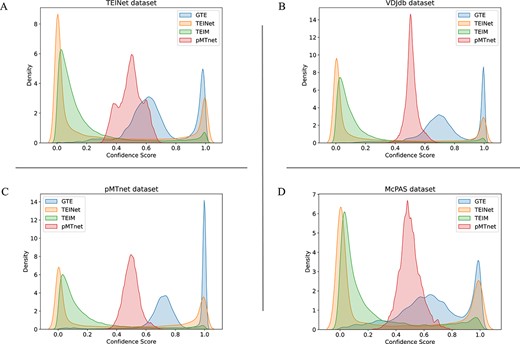
Confidence density on four datasets positive data; Panel A displays results for the TEINet Dataset, Panel B for the VDJdb Dataset, Panel C for the pMTnet Dataset, and Panel D for the McPAS Dataset.
Evaluation on independent dataset
To further compare the performance of each model, we use the independent test set provided by the baseline TEINet [16], referred to as PDB. This PDB test set collects 105 TCR–epitope complex structures from the public RCSB Protein Database (PDB) [50]. After filtering, it contains 63 positive samples. The PDB independent test set is a roughly balanced dataset, with each epitope binding to one or two TCRs. For a fair comparison, the TEINet dataset is used as the training set. Specifically, we generate a 1:1 ratio of negative samples following the StrictTCR partitioning. The same approach applies to the PDB independent test set. During training, a five-fold cross-validation method is employed, where one fold is used for validation and model selection. The final report presents the results from five iterations of the independent test set. As shown in Fig. 6, the results indicate that the AUC of the GTE model is higher than the baselines, demonstrating the powerful capability of utilizing graph topological structures.
Confidence density
In a bid to bolster the reliability of our findings, we proceeded to conduct a confidence analysis of the predictions across the four datasets. We employ Kernel Density Estimation (KDE) [51], a technique for estimation of probability density function. This method smooths the distribution of confidence scores without assuming any specific distribution shape. This flexibility arising from its nonparametric nature makes KDE a very popular approach for data drawn from a complicated distribution. The prediction results are model output logits, distributed between 0 and 1. Figure 7 displays the confidence density distributions of positive samples within these datasets. A distribution closer to 1 signifies higher confidence. However, TEINet and TEIM tend to predict most positive sample data as below 0.2, misclassifying them as negative samples. Our method exhibits higher confidence for positive sample predictions compared with all baseline methods, indicating that our model can easily distinguish positive samples and achieve high-confidence predictions, highlighting the superiority of our graph-based topological structure.
An interesting observation is that pMTnet predicts almost all data to be between 0.4 and 0.6. This behavior results from the “Differential loss function” used in pMTnet [8], aiming to ensure that positive samples score higher than negative ones, but does not concentrate on bringing positive samples close to 1 and negative samples close to 0. Conversely, other methods apply the Cross Entropy loss [52], and therefore, their predictions work toward making positive samples close to 1 and negative samples close to 0.
Limitations
TCR–epitope prediction holds great potential for advancing immunotherapy development [25]. Public databases accumulate increasingly more data on TCR–epitope interactions. Benefiting from these data, researchers develop various prediction frameworks based on deep learning algorithms. GTE is a novel approach that uses graph topological structures to capture the potential structural information between TCRs and epitopes, which provides a new perspective for TCR epitope prediction. However, one potential limitation is that GTE follows other SOTA methods to use the CDR3 region of the TCR’s beta chain, while previous work has shown that data containing only CDR3.|$\beta $| information are of lower quality compared with data that include paired CDRs [6, 53]. Incorporating the full TCR information presents a challenge, which will be the focus of our ongoing work. We plan to design a more comprehensive heterogeneous graph that includes information from both chains of the TCR to achieve accurate TCR specificity prediction.
Conclusion
We present GTE, an innovative framework that leverages graph topological structures to improve the prediction of TCR–epitope binding. Our method tackles the challenges of negative sample utilization and data imbalance through dynamic graph learning and AUC maximization strategies. Extensive experiments on four datasets demonstrate the promise of graph-based topological methods in predicting TCR–epitope interactions and offer valuable perspectives on the complex molecular networks underlying immune responses.
We introduce GTE, which is the first method leveraging topological structure to enhance TCR-epitope binding predictions through an inductive heterogeneous GNN.
We develop an advanced dynamic graph learning mechanism for adaptive negative data sampling during training, allowing efficient learning without memory limitations.
We adapt AUC maximization in the graph domain to ensure our model maintains a balanced and robust predictive capability, overcoming the challenge of data imbalance.
Funding
This work was partially supported by US National Science Foundation IIS-2412195, CCF-2400785, the Cancer Prevention and Research Institute of Texas (CPRIT) award (RP230363), the National Institutes of Health (NIH) [R01CA258584/TW], and Cancer Prevention Research Institute of Texas [RP230363/TW].
Data and code availability
GTE is implemented in Python using Pytorch. All the data and code are available at https://github.com/uta-smile/GTE.
References
