


Abstract
Protein complexes are key functional units in cellular processes. High-throughput techniques, such as co-fractionation coupled with mass spectrometry (CF-MS), have advanced protein complex studies by enabling global interactome inference. However, dealing with complex fractionation characteristics to define true interactions is not a simple task, since CF-MS is prone to false positives due to the co-elution of non-interacting proteins by chance. Several computational methods have been designed to analyze CF-MS data and construct probabilistic protein–protein interaction (PPI) networks. Current methods usually first infer PPIs based on handcrafted CF-MS features, and then use clustering algorithms to form potential protein complexes. While powerful, these methods suffer from the potential bias of handcrafted features and severely imbalanced data distribution. However, the handcrafted features based on domain knowledge might introduce bias, and current methods also tend to overfit due to the severely imbalanced PPI data. To address these issues, we present a balanced end-to-end learning architecture, Software for Prediction of Interactome with Feature-extraction Free Elution Data (SPIFFED), to integrate feature representation from raw CF-MS data and interactome prediction by convolutional neural network. SPIFFED outperforms the state-of-the-art methods in predicting PPIs under the conventional imbalanced training. When trained with balanced data, SPIFFED had greatly improved sensitivity for true PPIs. Moreover, the ensemble SPIFFED model provides different voting schemes to integrate predicted PPIs from multiple CF-MS data. Using the clustering software (i.e. ClusterONE), SPIFFED allows users to infer high-confidence protein complexes depending on the CF-MS experimental designs. The source code of SPIFFED is freely available at: https://github.com/bio-it-station/SPIFFED.
INTRODUCTION
Cellular processes and regulatory mechanisms are highly dependent on stable protein–protein interaction (PPI) networks, in which certain interacting proteins can form protein complexes to execute specific functions [1]. Elucidating the interactome structure is key to understanding proteome organization and its role in disease [2, 3]. Due to advances in high-throughput technologies [4–6], including binary PPI technologies [7–9], affinity purification/mass spectrometry (AP-MS) [10–12] and co-fractionation/mass spectrometry (CF-MS) [13–15], partial reconstruction of protein interactomes in many organisms has now been achieved. Compared to binary interaction techniques and AP-MS, which require protein tags to help identify target-related interactions, CF-MS is a more flexible and efficient technique to simultaneously study the entire interactome under native conditions [6]. However, dealing with complex fractionation characteristics to define true interactions is not a simple task [16–19].
Two computational methods, PrInCE [20] and EPIC [21], were specifically designed to standardize automated analysis of CF-MS data and construct probabilistic PPI networks from experimental data. The basic contents of these two approaches are similar, including optional machine learning classifiers [i.e. support vector machines, naive Bayes, logistic regression and random forest (RF)], several similarity metrics (such as Pearson correlation, Euclidean distance, co-apex, etc.) for feature construction and database-defined reference sets for training data curation. While powerful, these methods still leave room for improvement. For example, the PPI data is usually severely imbalanced [22], with the number of positive PPIs an order of magnitude less than that of negative PPIs. This makes the model weaker for feature learning with positive PPI and less sensitive to noise with negative PPI, resulting in model overfitting. However, none of these computational methods have specifically addressed the problem of data imbalance. In addition, the manually defined similarity metrics (i.e. handcrafted features), although carry a certain degree of useful information, have limitations in the representation of latent information, partly require time-consuming calculations and are sensitive to the noise of data.
One way to overcome the problems raised by handcrafted features is end-to-end learning, a technique in which the model learns everything between input and output, and thus the handcrafted features are not necessary. The architectures of multi-layer neural networks (NNs) are by nature end-to-end learning that can improve the issue of feature extraction [23, 24]. The NN structure blurs the lines between learning and other processing modules, enabling feature learning to be optimized in an efficient coherent process. Meanwhile, multiple nonlinear transformations in NNs convert raw data into highly invariant and distinguishable representations, amplifying hidden information and reducing the impact of data noise [25–27]. To improve the current computational analysis of CF-MS data, we proposed an end-to-end learning approach: Software for Prediction of Interactome with Feature-extraction Free Elution Data (SPIFFED), which uses Convolutional Neural Networks (CNNs), one of the most popular NN architectures, for feature extraction and PPI classification. To evaluate the performance of SPIFFED, we compared it to EPIC under the same pre-processing steps. Furthermore, we addressed the problem of data imbalance by examining the model performance of SPIFFED for different levels of data imbalance. Finally, to integrate predictions from multiple data, we also added an ensemble model to SPIFFED that not only screens out predictions with high confidence, but whose results also reflect the abundance and consistency of predictions across data.
![The main components of SPIFFED. (A) Pre-processing features by pairing protein co-elution profiles. (B) Labeling PPIs with the reference complex set. (C) Training a CNN for PPI classification and evaluating its classification performance. (D) Integrating predicted positive PPIs [PPIs (+)] from multiple data for (E) subsequent clustering and complex prediction. Solid line: positive prediction, dash line: negative prediction.](https://oup.silverchair-cdn.com/oup/backfile/Content_public/Journal/bib/24/4/10.1093_bib_bbad229/1/m_bbad229f1.jpeg?Expires=1749262531&Signature=tjhzWypdcFRd8ldA6KSGhgCy94egHL9R7~NHNqW5TlaTux1GQzQCMX6wpK1KMOfUdP8ZVaS8rzzQeduDJ5pF1MI7dOFjOh-KgKLXQmAxfLLgV~xPjzHsQuCQWnYaep1tFM6~fIFUeYl094BTjcjYT-PzzWxdWSvCDWkungSEbFQUVDbemtKfMLXtDmmBCIGiTojvy05efeuwvVqsr0lfrInRwPXmXrEAN4j2yEFMWgQmsRQdb2j2HRaI1MBgPX9qZZ2jpf1uBFZD4ivAve7Gv2yp2m3J1WigpiN~XF~rn2wrB7VLdXG-9CpFhgfHa4eNkPXy2ls-t8BdlZpvegN2qQ__&Key-Pair-Id=APKAIE5G5CRDK6RD3PGA)
The main components of SPIFFED. (A) Pre-processing features by pairing protein co-elution profiles. (B) Labeling PPIs with the reference complex set. (C) Training a CNN for PPI classification and evaluating its classification performance. (D) Integrating predicted positive PPIs [PPIs (+)] from multiple data for (E) subsequent clustering and complex prediction. Solid line: positive prediction, dash line: negative prediction.
RESULTS
Performance comparison of SPIFFED with EPIC
We constructed an end-to-end learning approach, SPIFFED, with considering feature extraction-free and balance training to infer protein complexes from CF-MS data (Figure 1). To evaluate its performance, we first compared SPIFFED on PPIs with a well-established model, EPIC, under the same conditions (Figure 2A). Overall, SPIFFED outperforms EPIC in all metrics for both worm and yeast dataset. The average accuracy, average area under the curve of receiver-operator characteristic (AUC of ROC) and average area under the curve of precision and recall (AUC of PR) of SPIFFED on the testing set are 0.03, 0.08 and 0.14 higher than those of EPIC, respectively. In addition, the performance difference between training and testing of accuracy, AUC of ROC and AUC of PR for SPIFFED are 0.09, 0.14 and 0.29 lower than those of EPIC, respectively, indicating that SPIFFED has learned a more generalized feature representation than EPIC.
Since there is a significant difference in AUC of PR between the two models, we further examined the precision and sensitivity of these models on the testing set and found that SPIFFED surpassed EPIC in both average precision (EPIC: 0.66, SPIFFED: 0.71) and average sensitivity (EPIC: 0.33, SPIFFED: 0.54), especially in the latter comparison (Figure 2B). The fact that SPIFFED and EPIC have comparable precision but different sensitivity suggests that SPIFFED is superior to EPIC mainly due to a higher proportion of correctly classified positives (true positives), as shown in the confusion matrix (Figure 2C).
Overall, our results show that SPIFFED outperforms and generalizes better than EPIC. Although SPIFFED has a more balanced predictive performance than EPIC, it is still skewed toward making negative classifications, which leaves room for improvement especially for sensitivity.
The impact of data imbalance on model performance
The skewed classification observed in Figure 2 is most likely caused by the imbalanced training data since a 1:5 ratio of positive and negative samples was used to train the model. To improve the skewed classification problem, we randomly down-sized negative samples for training and examined the effect of different proportions of positive to negative samples on the model’s performance.
When the ratio of positive to negative samples in the training set was changed from 1:5 to 1:2 and 1:1, SPIFFED’s average sensitivity increased substantially (from 0.74 to 0.85 and 0.91 on the training set and from 0.54 to 0.69 and 0.78 on the testing set; Figure 3A), as the true positives increased (Figure 3B). Average precision also improved slightly (from 0.88 to 0.89 and 0.91 on the training set, and from 0.71 to 0.74 and 0.77 on the testing set; Figure 3A), as the increase of true positives outweighed the increase in false positives (Figure 3B). As a result, average F1 score, which is a composite metrics measuring both the performance in sensitivity and precision, also increased (from 0.80 to 0.87 and 0.91 on the training set, and from 0.61 to 0.71 and 0.78 on the testing set, Figure 3A), indicating that optimal performance in predicting positive interactions is achieved with balanced training data. However, average specificity decreased (from 0.98 to 0.95 and 0.91 on the training set, and from 0.96 to 0.88 and 0.77 on the testing set; Figure 3A) due to the decrease of true negatives (Figure 3B). This complementary change in the predictive power for positive and negative interactions resulted in no obvious change in Matthews correlation coefficient (MCC) (from 0.77 to 0.81 and 0.81 on the training set, and from 0.56 to 0.58 and 0.55 on the testing set), which is a comprehensive metric that can simultaneously consider a model’s performance in correctly predicting the positives and the negatives. Nevertheless, the increase in average sensitivity outweighed the decrease in average specificity as the proportion of positive to negative samples in the training set gets closer. Our results show that the optimal training condition is achieved when the proportion of positive to negative samples in the training set is equal, in which case the model has the most balanced predictive power.
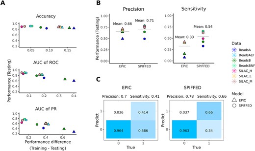
Comparison of SPIFFED and EPIC on model performance. (A) The classification performance of the model on the testing set was evaluated from accuracy, AUC of ROC, and AUC of PR, and the performance difference between the training set and the testing set. (B) Comparison of the precision and sensitivity of the two models on the testing set. (C) Taking the confusion matrix of BeadsBNF (testing set) as an example, when the difference in sensitivity between the two models is greater than precision, the difference in their classification performance is mainly reflected in the judgment of positive predictions.
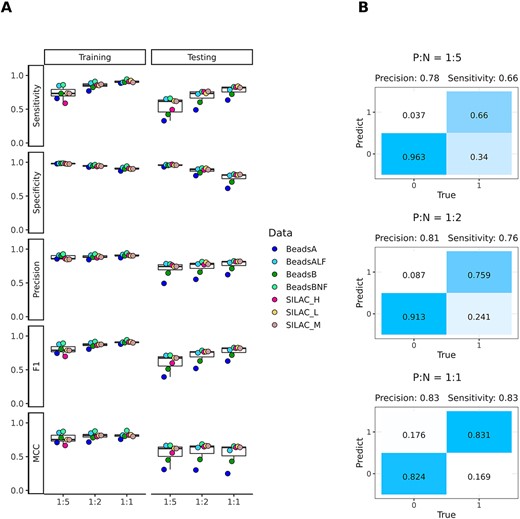
The impact of data imbalance on SPIFFED’s predicting power. (A) Variation of model classification performance on training set and testing set under the influence of different proposition of positive and negative samples. (B) Taking the confusion matrixes of BeadsBNF (testing set) as an example, as the ratio of positive and negative samples increases, the prediction ability of SPIFFED for the two classes gradually reaches a balance.
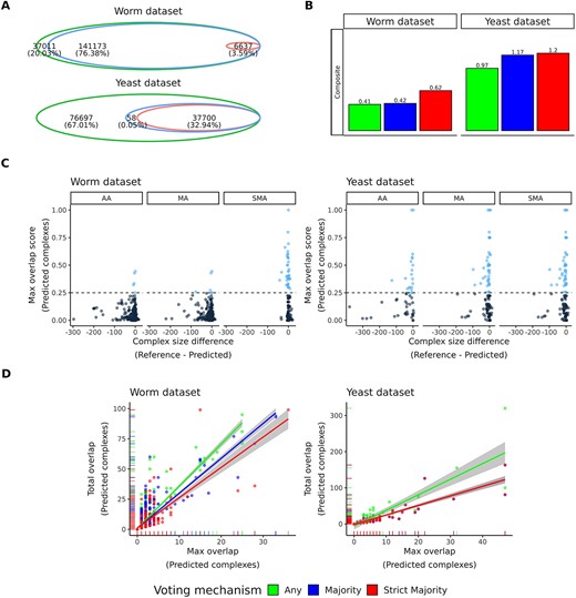
Integrate predictions from multiple data using SPIFFED’s ensemble model. (A) The intersection of positive PPIs under the screening of three voting mechanisms in the ensemble model. (B) Evaluating the composition of predicted complexes constructed from positive predictions screened by different voting mechanisms. (C) Relationship between maximum overlap score and size difference for each pair of predicted and reference complexes. The dashed line is the overlap score threshold (0.25), and the light blue dots are the predicted clusters that pass the threshold, which are then considered for Overlap calculations. (D) Relationship between maximum and total overlaps between predicted complexes and reference complexes. In the result of yeast data, the regression line of MA is too close to SMA and cannot be observed directly.
Integrate positive predictions across data via SPIFFED’s ensemble model
We further developed a SPIFFED’s ensemble model to integrate the positive predictions generated from different data. Three voting mechanisms, Any Agreement (AA), Majority Agreement (MA) and Strict Majority Agreement (SMA), were used to select for different levels of prediction consistency (see Materials and methods). Here, all pair-wise protein pairs in each experimental data were used to train the corresponding models, and all PPIs predicted by the models (including positive, negative and indeterminate PPIs) were used for subsequent cluster analysis. Figure 4A shows the intersection of positive predictions produced by the three voting mechanisms. In the worm dataset, a total of 184 821 positive predictions were integrated, of which ~80% passed MA screening and ˂4% passed SMA screening. In the yeast dataset, there were 114 455 positive predictions, of which MA and SMA screened positive predictions accounted for 32.99% and 32.94%, respectively. These results suggest that positive predictions from the worm dataset are mostly disjoint across the data, while those supported by more than half of the data are rare. In contrast, about one-third of the positive predictions in the yeast dataset were consistent across more than half of the data (Figure S1 and Table S1).
To assess the impact of different voting mechanisms on the subsequent analysis of PPI, we used the integrated positive predictions to generate predicted complexes and evaluated their structural composition against the reference protein complexes. As shown in Figure 4B, SMA received the highest composite scores (see Materials and methods) in both datasets. By examining the components of the composite score, we found that the differences among the three voting mechanisms were mainly driven by the proportion of intersections between the predicted complex and the reference complex (as measured by overlap score), as well as the specificity of the intersection (as measured by PPV). Complexes inferred using MA and AA on the worm dataset and AA on the yeast dataset are generally larger than the reference complexes (negative on the x-axis), thus reducing the proportion of intersections (lower y-axis distribution) (Figure 4C). In addition, these complexes can also be mapped to multiple reference complexes, resulting in low specificity for intersections (low maximum overlap and high total overlap, hence high slope of linear relationship) (Figure 4D). Correspondingly, the voting mechanisms that inferred these complexes also had lower composite score (Figure 4B).
The above results demonstrate that the intersection of the SPIFFED’s ensemble model results can reflect the abundance and consistency of predictions across different data. Furthermore, we found that SMA-inferred complexes had the highest composite scores in both datasets, reflecting its ability to filter out low-confidence PPIs and subsequently prevent the generation of oversized or nonspecific protein complexes during the clustering process.
DISCUSSION
Our results present a pioneer study to analyze PPIs from CF-MS data using an end-to-end machine learning architecture. The entire feature learning process of SPIFFED is done through CNN, where convolutional layers are used for feature extraction and NNs are used for layer-wise abstraction. SPIFFED outperforms the commonly used multi-step learning model (EPIC) in all metrics for both the worm and the yeast dataset (Figure 2), suggesting that the features learned by our model better reflects the differences between positive and negative PPIs than manually defined features used in EPIC. In recent years, similar end-to-end approaches have been applied to analyze continuous signal data [28, 29] and continuous biological data [30–32]. These studies have successfully transformed the local information into an efficient feature representation by the model and thus achieves better performance in the final task. In this study, we demonstrated that SPIFFED is a conceptually and results-supported model that outperform existing CF-MS analytical methods.
Although powerful, SPIFFED still faces the data imbalance issue in the PPI prediction. Training a model with imbalanced data resulted in predictions that better reflects the class distribution of the real data, which is dominated by non-interaction pairs. The model from imbalanced data has high predictive power for non-interaction pairs (i.e. high specificity) but low predictive power for true interactions (i.e. sensitivity) due to the skewed predictions (Figure 2). However, since the goal of CF-MS experiments is to obtain a more complete protein interactome map by predicting unknown interactions from a small set of gold standards, predictive power for true interaction is more important here. Newly predicted unknown interactions provide material for further experimental validation. A slight increase in false positive rate is also acceptable as the prediction becomes balanced. Some of ‘non-interactions’ defined from gold standards are potentially positives because the interaction might be too weak to be detected by previous experimental assays. Therefore, it is not necessary to trade the predictive power on true interactions for non-interactions. In fact, the data imbalance is a common issue in machine learning on biological data, such as protein interaction sites prediction [33], drug discovery [34] and so on. To address this issue, some methods are proposed, for example sampling techniques (down-sampling and up-sampling), cost-sensitive classifiers, etc. In this study, we constructed the balanced training data by randomly down-sampling non-interaction pairs. Our results (Figure 3) show that SPIFFED is more sensitive to true interactions when the data becomes more balanced, with losing limited specificity.
As SPIFFED achieves a more balanced classification, more positive predictions are also made. In order to filter out positive interactions with low confidence, SPIFFED provides an ensemble model that can integrate the predictions from different data. The intersection of the three voting mechanisms of the ensemble model provides rich information (Figure 4 and Table S1): a high intersection between the two majority-based voting mechanisms (i.e. MA and SMA) reflects a high consistency of protein interaction information across data. We showed that protein complexes clustered from high-confidence PPIs resulted from the strictest voting mechanism (i.e. the SMA mechanism) have higher composite scores than those clustered from low-confidence PPIs resulted from the voting mechanisms with relatively lower thresholds (i.e. the MA and AA mechanisms). These results demonstrate that SPIFFED’s ensemble model can effectively select high-confidence protein interactions to improve the performance of protein complex prediction. Moreover, if the CF-MS experiments are done in different conditions, the results from different voting mechanisms allow us to compare the stability of the interactions. The PPIs appears only in SMA are the most stable ones and those appear only in AA are the least. These results demonstrate that SPIFFED’s ensemble model can effectively select the high-confidence results and improve the performance of subsequent analysis.
The current version of SPIFFED’s ensemble model focuses on identifying PPIs (complexes) consistently found in CF-MS data obtained in diverse biological contexts. It is of interest to further identify differential PPIs (complexes) across different datasets. For example, we can apply SPIFFED to the comprehensive resource of CF-MS experiments across 27 eukaryotic species collected by Skinnider and Foster [35] to study the conserved and unique PPIs (complexes) in different species or clades. Since SPIFFED does not utilize any information other than CF-MS data, it can be easily extended to other species and tend to be more generalizable than methods requiring external data source [36]. In addition, without using external data that is invariant under changes, SPIFFED will be sensitive in capturing the dynamics between snapshots of protein interactome from multiple-condition data. By identifying confident protein complexes in different conditions, we can analyze how these complexes change in response to various growth conditions, including their components and function. However, mapping the corresponding complexes in different conditions is challenging, particularly when optimal matchings for all complexes are preferred. In the future, we plan to extend SPIFFED to identify differential and dynamic PPIs (complexes) across datasets. This will require the development of new algorithms and statistical analysis methods.
In conclusion, we demonstrate that SPIFFED is a robust tool that can handle various shapes and shifts of signals in co-fractionation data and learn more general feature representations through an end-to-end structure. With a balanced training set, SPIFFED can accurately identify true interactions from a large number of non-interactions and assign the confidence level of predictions across data through an ensemble model.
MATERIALS AND METHODS
Overview
SPIFFED is a supervised machine-learning pipeline that performs elution profile-based inference of PPIs. SPIFFED takes protein elution profiles as features directly without any other dedicated feature extraction step (Figure 1A). Labels are generated from reference protein complexes (Figure 1B) [37]. To facilitate a fair comparison, most of the implementation from the protein complex prediction tool, EPIC [21], were used for these pre-processing steps. SPIFFED uses processed elution profiles and labels to train a CNN (Figure 1C). Evaluation results are provided for each trained model, allowing users to evaluate the model before using it for new PPI predictions. SPIFFED also includes the option to combine multiple trained models (Figure 1D) and is followed by a downstream module for clustering the predicted PPIs into protein complex (Figure 1E).
Datasets
We used three datasets to evaluate the performance of SPIFFED, including a published human cells protein dataset used in evaluating PrInCE [20], a published dataset of worm protein profiles used in evaluating EPIC [21], and a dataset we generated from yeast proteins (hereafter as ‘the human dataset’, ‘the worm dataset’ and ‘the yeast dataset’, respectively). The human dataset contains two elution profiles, condition 1 and condition 2 (in this study we used the replicate 1 from each condition), downloaded from https://github.com/fosterlab/PrInCE-Matlab/tree/master/Input. The worm dataset contains four elution profiles, beadsA, beadsALF, beadsB and beadsBNF, downloaded from https://github.com/BaderLab/EPIC. The yeast dataset contains three elution profiles, namely SILAC_H, SILAC_M and SILAC_L, and the mass spectrometry proteomics data have been deposited to the ProteomeXchange Consortium via the PRIDE [38] partner repository with the dataset identifier PXD031967. The detailed experimental processes of yeast dataset are described in Supplemental Materials. After we determined the generalizability of SPIFFED on the datasets of these three very different species (Supplementary Table S2), we focused on the results of the worm and the yeast datasets only for simplicity. Since different elusion methods were used to generate the worm dataset, the overlapping information between the data was low. The experimental conditions for generating the yeast dataset were similar, so the data were similar to biological replicates. The number of proteins in these two datasets are shown in Table 1.
Number of proteins in the data before and after pre-processing
| Datasets | Data | Protein number (original) | Protein number (after filtering) |
|---|---|---|---|
| Worm | BeadsA | 5565 | 2704 |
| BeadsALF | 4550 | 2331 | |
| BeadsB | 5007 | 2743 | |
| BeadsBNF | 4822 | 2589 | |
| Yeast | SILAC_H | 2059 | 1963 |
| SILAC_M | 2059 | 1962 | |
| SILAC_L | 2059 | 1962 |
Data pre-processing
Elution profile pre-processing
Protein elution profiles were formatted as a M × N matrix, with M proteins and N fractions first be normalized by column and then by row. Column-wise normalized values Ci,j and row-wise normalized values Ri,j were calculated by:
where Ei,j represents the signal of protein i in fraction j.
Pre-processing of reference protein complexes
Reference protein complexes were first trimmed by removing proteins with no elution profile presence in the experimental data. Similar to EPIC, the remaining complexes whose size exceed 50 or less than three were filtered out to reduce the potential bias. The final reference set used for analysis contained trimmed protein complexes with all constituent members having experimental data.
Protein pairs creation and labeling
To have a fair comparison, we followed the protein pairs filtering step defined in EPIC. First, all possible pair-wise protein pairs in the list of elution profiles were generated. Those pairs that never occurred in the same fraction were removed. Then, we used the co-elution score (Pearson correlation) to filter out the protein pairs with a score lower than 0.5. The numbers of proteins in the two datasets after pre-processing are shown in Table 1. The remaining protein pairs were assigned to one of the three labels, ‘positive PPI’, ‘negative PPI’ and ‘unsure PPI’. Positive PPI was defined as two proteins that were found together in a reference protein complex. Negative PPI refers to a protein pair present in two different reference complexes. As for PPIs that matched to none or only one constituent protein of any reference complexes, they were labeled as unsure PPIs.
CNN model training and evaluation
Model architecture
SPIFFED uses CNN to extract features and learn meaningful feature representations from the pair-wise elution profile of PPIs. There is no additional feature extraction step in between elution profiles pre-processing and CNN model training. The detailed layer architecture and hyperparameters of CNN are shown in Table S3, and we used the yeast dataset to demonstrate the output shape.
Model evaluation
The evaluation model was trained and evaluated by all positive PPIs and a subset of negative PPIs, with a positive to negative ratio equaling to 1:5. We applied 5-fold cross-validation for model evaluation. In each fold, one split was held out as the testing dataset and a model was trained on the remaining four splits. We evaluated the trained model in each fold by making predictions with both the training splits and the testing split, and the results calculated from these predictions were referred to as ‘training performance’ and ‘testing performance’, respectively. After five iterations, the prediction results were aggregated to calculate the accuracy, area under curve for receiver-operator characteristic and precision-recall (AUC of ROC and PR), precision, sensitivity, F1 score and MCC to provide evaluation at multiple aspects. The evaluation metrics were defined as
where TP, TN, FP, FN refer to true positive, true negative, false positive and false negative, respectively.
Comparison with EPIC
We compared the performance of SPIFFED with the two leading tools in the field, PrInCE and EPIC. EPIC outperformed PrInCE in our initial evaluation (Supplementary Table S2), so we focused our subsequent comparisons with EPIC only for simplicity. We evaluated EPIC’s best-performing model, RF, with the optimized set of calculated features (Mutual Information, Bayes correlation, Euclidean distance, Apex and weighted cross correlation) selected in the original paper [21]. After feature extraction and selection steps, each protein pair was reduced to five values. We trained the RF model using the EPIC software with default parameters but evaluated the performance using our evaluation scheme outlined in the previous section. Our evaluation scheme put emphasis on comparing the difference between training performance and testing performance, which is important in training a model that generalizes well with new data.
Effect of class imbalance on model training
To evaluate whether we could achieve a more balanced performance in predicting positive and negative labels, we trained models with different degrees of data imbalance using the same parameters. In addition to the original training dataset with a 1:5 positive to negative ratio, we prepared two other training datasets with 1:2 and 1:1 positive to negative ratios by further down sampling the negative PPIs.
Ensemble model and clustering of PPIs
Ensemble model
SPIFFED provides a module for users to build an ensemble model that can obtain confident positive PPIs based on the consistency of the positive predictions across multiple data. The ensemble model module includes three optional voting mechanisms, namely AA, MA and SMA. AA collects all positive PPIs that appear in predictions, so it has the greatest number of PPIs compared to the other two voting mechanisms. MA collects those PPIs whose positive occurrences are in at least half (≥0.5) of the total occurrences (i.e. not counting data without available prediction). SMA collects positive PPIs with occurrences in at least half (≥0.5) of the data, and hence only those high-confidence predictions are retained. Therefore, the collected positive PPIs by SMA is a subset of that by MA, and the collected positive PPIs by both SMA and MA are subsets of that by AA. Table S1 shows the conditions for passing the three voting mechanisms when the number of data is four.
Clustering and evaluation
The software ClusterONE [39] was used to cluster the PPIs into predicted complexes through the confidence scores generated by the classifier. Four cluster evaluation metrics, including Overlap, positive predictive value (PPV), Sensitivity and maximum matching ratio (MMR) were used in this study. These metrics measure compositional similarity between predicted and reference complexes from different perspectives. The Overlap, geometric mean of PPV and Sensitivity, and MMR were further summed into a composite score to examine the overall potential of the predicted complexes.
SPIFFED enables end-to-end learning from feature representation of co-elution data to protein interactome inference.
SPIFFED uses balanced training to reduce noise amplification and overfitting present in past analysis methods.
SPIFFED allows users assessing the consistency of multiple experiments and integrate them to obtain confident prediction.
FUNDING
This work was supported by Academia Sinica, Taiwan (AS-GC-110-L15) and the National Science and Technology Council, Taiwan (110-2221-E-001-013-MY3).
DATA AVAILABILITY
The source code for the SPIFFED is available on GitHub (https://github.com/bio-it-station/SPIFFED).
The mass spectrometry proteomics data of yeast dataset have been deposited to the ProteomeXchange Consortium via the PRIDE [36] partner repository with the dataset identifier PXD031967.
AUTHOR CONTRIBUTIONS STATEMENT
Y.-H.C. analyzed and interpreted the data, wrote the manuscript and prepared figures. K.-H.C. conceptualized the study, developed the algorithm and performed the benchmark experiments. C.-F.L. and J.Y.W. interpreted the data and revised the manuscript. J.-Y.L. and H.-K.T. supervised the project, reviewed and edited the manuscript.
Author Biographies
Yu-Hsin Chen is a PhD student in the Taiwan International Graduate Program Bioinformatics program organized by National Taiwan University and Academia Sinica. Her research focuses on bioinformatics and machine learning.
Kuan-Hao Chao is a PhD student for Computational Biology at Johns Hopkins University. His research interests are genome assembly and transcriptome (RNA sequencing). He is also passionate about developing open-source bioinformatics tools and designing algorithms.
Jin Yung Wong received the PhD degree in Biodiversity from the National Taiwan Normal University, Taipei, Taiwan, in 2020. He is a postdoctoral research fellow at the Institute of Information Science, Academia Sinica. His research interests include evolution, genomics, machine learning and biomechanics.
Chien-Fu Liu received the MS degree in Institute of Bioinformatics and Biosignal Transduction from National Cheng Kung University, Taiwan, in 2015. He is a research assistant at the Institute of Molecular Biology, Academia Sinica. His research interests include genomics, evolution, endosymbiosis and machine learning.
Jun-Yi Leu received the BS degree in Chemical Engineering from National Tsing Hua University, Hsinchu City, Taiwan and the PhD degree in Molecular, Cellular and Developmental Biology from Yale university, New Haven, CT, USA in 1988 and 1999, respectively. He is a distinguished research fellow at the Institute of Molecular Biology, Academia Sinica. His research interests include endosymbiosis, phenotypic robustness and genetic incompatibility.
Huai-Kuang Tsai received the BS, the MS and the PhD degrees in Computer Science and Information Engineering from the National Taiwan University, Taipei, Taiwan, in 1996, 1998, and 2003, respectively. He is a Research Fellow at the Institute of Information Science, Academia Sinica. His research interests include computational biology, bioinformatics, gene regulation and machine learning.
REFERENCES
Author notes
Yu-Hsin Chen and Kuan-Hao Chao contributed equally to this work and should be regarded as Joint First Authors.
