


Abstract
Precise targeting of transcription factor binding sites (TFBSs) is essential to comprehending transcriptional regulatory processes and investigating cellular function. Although several deep learning algorithms have been created to predict TFBSs, the models’ intrinsic mechanisms and prediction results are difficult to explain. There is still room for improvement in prediction performance. We present DeepSTF, a unique deep-learning architecture for predicting TFBSs by integrating DNA sequence and shape profiles. We use the improved transformer encoder structure for the first time in the TFBSs prediction approach. DeepSTF extracts DNA higher-order sequence features using stacked convolutional neural networks (CNNs), whereas rich DNA shape profiles are extracted by combining improved transformer encoder structure and bidirectional long short-term memory (Bi-LSTM), and, finally, the derived higher-order sequence features and representative shape profiles are integrated into the channel dimension to achieve accurate TFBSs prediction. Experiments on 165 ENCODE chromatin immunoprecipitation sequencing (ChIP-seq) datasets show that DeepSTF considerably outperforms several state-of-the-art algorithms in predicting TFBSs, and we explain the usefulness of the transformer encoder structure and the combined strategy using sequence features and shape profiles in capturing multiple dependencies and learning essential features. In addition, this paper examines the significance of DNA shape features predicting TFBSs. The source code of DeepSTF is available at https://github.com/YuBinLab-QUST/DeepSTF/.
INTRODUCTION
Transcription is the initial step in the expression of genes, which can be accelerated or inhibited by transcription factors (TFs) in conjunction with a particular sequence of DNA. Transcription factor binding sites (TFBSs) are DNA segments that bind to specific transcription factor (TF), generally ranging 4–30 bp [1–3]. Accurate prediction of TFBSs is critical for identifying unique core characteristics of the genome and understanding how highly specialized sequence expression programs are programmed in biological systems, assisting in the resolution of certain contemporary difficulties in molecular biology and medicine, and advancing systems biology and molecular biology [4–6]. Chromatin immunoprecipitation sequencing (ChIP-seq) [7] may identify DNA fragments interacting with transcription factors on a genome-wide scale, providing research with massive quantities of credible data on TFBSs. Nevertheless, ChIP-seq experiments sometimes necessitate using difficult-to-obtain reagents and materials, such as antibodies against certain TFs. As a result, utilizing computational approaches to predict TFBSs from sequences is not only efficient but also inexpensive, and it is now the most preferred solution [8, 9].
Several machine learning-based approaches for forecasting TFBSs have been developed, including the Hidden Markov model (HMM) [10], random forest model [11, 12], support vector machine (SVM) [13, 14] algorithms, etc. Although these algorithms perform well in the TFBSs prediction challenge, they rely on prior knowledge of sequence preferences and cannot automatically extract significant characteristics from the original input sequence.
Based on the current massive and trustworthy TFBSs data, deep learning computational approaches may make full use of the enormous quantity of experimental data to automatically learn relevant features from the original input sequence and have higher learning performance in predicting TFBSs compared with typical machine learning models. For example, SAResNet [15], DeepGRN [16] and DSAC [17] have improved TFBSs prediction performance by combining convolutional neural networks (CNNs) and attention mechanisms [18]. This illustrates that by combining CNN and attention approaches, improved deep network architecture can be developed to extract high-dimensional properties of the tied region, effectively enhancing the model’s prediction accuracy. The conformation and morphology of DNA molecules in three-dimensional space is known as DNA shape. An increasing body of research suggests that the interaction pattern between TFs and their specific binding sequences is highly conserved across species, and this conservation is closely linked to the three-dimensional spatial structure of DNA molecules. DNA shapes are critical in determining the DNA binding preferences of transcription factors and other DNA-binding proteins [19]. Hence, many approaches, including DLBSS [20], CRPTS [21], and D-SSCA [22], aim to integrate sequence and shape to enhance the accuracy of TFBSs prediction. Yet, these approaches do not entirely leverage the feature information obtained from sequences and shapes, there are limitations in knowledge discovery and interpretability, and prediction performance has a lot of space for improvement.
Recently, the Transformer model [23, 24] perfectly integrates feature and matching functions into the attention mechanism, achieving considerable success in natural language processing, computer vision and other domains [25–27]. The transformer model relies heavily on a multi-headed attention mechanism. Because of the redundant weights and the nonlinear relationship between input and output, deep neural networks are sometimes difficult to interpret. Still, the multi-headed attention mechanism is quite intuitive and interpretable [28]. Because the input contexts for utterance processing and DNA sequence processing are similar, we use analogous tactics to improve the TFBSs prediction model’s method performance.
Based on the above experience, we propose DeepSTF, a unique architecture integrating CNN, improved transformer encoder structure, and Bi-LSTM to combine sequence and shape to predict TFBSs. To validate the usefulness of the proposed model, we utilize the same datasets used in the work of Zhang et al. [22]. The experimental findings demonstrate that DeepSTF surpasses numerous state-of-the-art approaches in prediction performance. The average accuracy (ACC) for the test set of 165 ENCODE ChIP-seq datasets is 0.814. Overall, the key contributions of this study are divided into three categories: (i) DeepSTF, a novel multi-module hybrid deep learning architecture combining CNN, improved transformer encoder structure, and Bi-LSTM, is presented to combine DNA sequence and shape for TFBSs prediction. In addition, we explain the efficacy of sequence and shape features in capturing many dependencies and focusing on learning critical aspects. (ii) The improved transformer encoder structure is employed to predict TFBSs for the first time. The multi-head attention mechanism achieves a more comprehensive high-level representation of input information learned in different representation subspaces, and the module is interpretable. In addition, the impact of different attention mechanisms in TFBSs prediction is examined in depth in this paper. (iii) The detailed research and analysis of the ENCODE ChIP-seq datasets prove the feasibility of the proposed DeepSTF model. We offer an in-depth examination of the significance of DNA shape structure information predicting the TFBSs.
MATERIALS AND METHODS
Benchmark datasets
DNA sequence
We utilize the same datasets used in the work of Zhang et al. [22] to evaluate the performance of DeepSTF objectively. Specifically, 165 ChIP-seq datasets are acquired from the encyclopedia of DNA elements (ENCODE) project’s 690 ChIP-seq datasets, which span 29 TFs from diverse cell lines. Supplementary Table S1 details all cell lines and source organism information. Zeng et al. separated the 165 ENCODE ChIP-seq datasets into a training set and a corresponding test set in their work [29]. Each training subset (testing subset) is composed of a positive subset and a corresponding negative subset. The positive subset is made up of 101 bp DNA sequences that have been shown in biological investigations to have at least one transcription factor binding event, whereas the negative subset was created by rearranging the positive subset by matching the dinucleotide composition [30]. The ‘fasta-dinucleotide-shuffle’ package in MEME [31] is used for rearranging. Supplementary Table S2 displays detailed statistics, and Supplementary Table S3 shows the specific number of positive and negative samples for each dataset. All datasets are accessible at http://cnn.csail.mit.edu/motif_discovery/.
DNA shape
We considered computational complexity, model interpretability, and data availability, with the hope of achieving better performance while maintaining model simplicity. After investigating numerous structural properties of DNA, the following five typical shape features are chosen: helix twist (HelT), minor groove width (MGW), propeller twist (ProT), rolling (Roll), and minor groove electrostatic potential (EP). These features represent different aspects of DNA shape features that cover important information about DNA structure and function, and play a key role in the identification and regulation of TFBSs. The mechanisms by which transcription factors bind to DNA can be better understood by analyzing these shape properties. In addition, these features are easily accessible and computationally inexpensive, allowing us to use large amounts of data for research, and to compare and validate results with other studies. DNAshapeR is a R/BioConductor package for ultra-fast, high-throughput prediction of DNA shape features, valuable for analyzing large genomic datasets. It can predict, visualize and encode DNA shape features for statistical learning. Supplementary Table S4 describes the meaning of the main items in DNAshapeR and related resources, which can be obtained from http://www.bioconductor.org/ for DNAshapeR and a tutorial on its use.
Model description
The general architecture of DeepSTF is depicted in Figure 1.
Data pre-processing
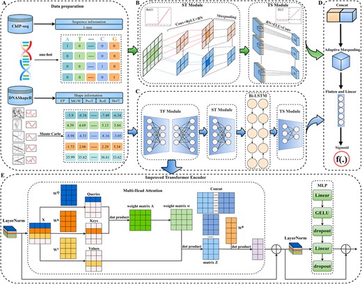
The DeepSTF framework in general. (A) Data pre-processing: DNA sequence and shape profiles are transformed into feature matrix. (B) Sequence clade processing: capture higher-order characteristics in multidimensional sequence profiles. (C) Shape clade processing: extract possible characteristics from multidimensional shape profiles. (D) Output processing: feature mapping is transformed into the final prediction. (E) TF Module: the improved transformer encoder structure's comprehensive processing flow.
DNA sequence: Using one-hot encoding, the 101 nucleotides of each input DNA sequence are mapped to the potential feature space. Base pairs A, T, C and G are represented as a one-hot vector for a specific DNA sequence, namely |$\left[1,0,0,0\right]$|, |$\left[0,1,0,0\right]$|, |$\left[0,0,1,0\right]$| and |$\left[0,0,0,1\right]$|. As a result, the sequence is represented as a feature matrix |${S}_1$| of dimension |$1\times 4\times 101$|, which can be seen as follows:
where |${M}_i$| refers to the one-hot vector of the ith nucleotide.
DNA shape: The Monte Carlo simulation package DNAshapeR is used to produce the structural feature distributions of the five individual nucleotides: HelT, MGW, ProT, Roll, and EP. The shape profiles for a specific DNA sequence are represented as a feature matrix |${S}_2$| of dimension |$1\times 5\times 101$|, as described in the following:
where |${N}_i$| means the Monte Carlo simulation vector of the ith nucleotide. The model data pre-processing process is illustrated in Figure 1(A).
Sequence clade processing
ST Module: Although convolutional operations may rapidly learn higher-order complex characteristics of DNA sequence, the performance of different convolutional designs varies greatly, and a large number of stacked convolutional networks can raise the learning complexity of the model and easily lead to gradient disappearance or gradient explosion. To obtain a more comprehensive representation of the higher-order features of the input sequence while avoiding the problem of having too many training parameters, this study first learns the higher-order complex features of the sequence using one convolutional operation and a rectified linear activation function (ReLU). Following that, the batch normalization method is used to correct the mean and variance in tiny batches to learn the proper offset and scaling to increase the model’s convergence speed and prevent overfitting while maintaining model accuracy. Furthermore, we use the max-pooling layer to pick the best response in the immediate neighboring region by preserving the maximum value within the window, subsampling the higher-order features to eliminate redundant information, and ultimately collecting the higher-order feature mapping |${E}_1$| derived by this module from the sequence. Technically, the module operation is as follows:
where |${W}_c$| signifies the convolutional layer’s weight matrix and |${b}_c$| denotes the convolutional layer’s bias. |$Conv\left(\ast \right)$| denotes the convolution procedure, |$BN\left(\ast \right)$| represents batch normalization operation, and |$Maxpool\left(\ast \right)$| represents local max-pooling action. The detailed architecture of the sequence clade ST Module is depicted in Supplementary Table S5.
TS Module: To gain richer feature information, the module initially performs a batch normalization procedure to normalize the features obtained from the ST Module. Then, exponential linear units (ELU) are employed to get the gradient closer to the natural gradient while boosting network resiliency. Lastly, a two-dimensional convolution operation is employed to generate a higher-order feature mapping |${P}_1$| with a tighter sequence. The module operation is specified formally as follows:
where |$BN\left(\ast \right)$| denotes the batch normalization process and |$Conv\left(\ast \right)$| the convolution operation. The specific design of the sequence clade’s TS Module is depicted in Supplementary Table S6. The sequence branch processing flow is depicted in Figure 1(B).
Shape clade processing
TF Module: This module is composed of a modified transformer encoder structure. To avoid the gradient expanding or vanishing, the input shape profiles |${S}_2$| across features are first adjusted using the layer normalization approach to provide distinct feature mappings |$X$| for the same sample. Formally, the calculation is as follows:
where |$LN\left(\ast \right)$| represents the layer normalization operation.
After that, to learn a complete high-level representation of shape feature information in multiple representation subspaces, this work refers to the notion of the most prominent encoder-decoder module [32, 33] in computer vision. First, a multi-headed attention mechanism is employed to learn the interdependence of distinct ranges of input information in multiple representation subspaces. Using the residual connection, the output of the layer normalization module is merged with the feature high-level representation provided by the multi-headed attention mechanism to generate a feature matrix |$F$| that achieves a gradient that stays apparent while decreasing information loss. The formal calculation procedure for this phase is shown in Supplementary S1. Next, |$F$| is normalized to a typical normal distribution using the layer normalization operation to prevent model overfitting and to keep the gradients visible. The MLP module is utilized to do feature transformation and information restructuring. The MLP module has two linear layers: the first doubles the amount of input nodes, whereas the second returns to the original number of nodes. The first linear layer is followed by a Gaussian Error Linear Unit (GELU), which allows the network to have nonlinear fitting capability while also incorporating the principle of regularization to increase the network’s generalization capability. A dropout operation is added before and after the second linear layer to increase training speed and minimize overfitting. Finally, the MLP module output is merged with the matrix |$F$| to produce the final output of the TF Module |$L$|. The exact calculation procedure is as follows:
The general processing flow of the TF Module is depicted in Figure 1(E), and the detailed design is depicted in Supplementary Table S7. Then, similar to the sequence branch processing, an ST Module is performed on |$L$| to obtain the fine output |${E}_2$|. The precise design of the ST Module of the shape clade is shown in Supplementary Table S8. Following that, the Bi-LSTM module is used to access the contextual information by combining the feed-forward hidden layer and the feed-back hidden layer to obtain the output |${E}_3$| with more extensive feature information. The formal computational procedure of Bi-LSTM is shown in Supplementary S2. The feature matrix |${E}_3$| is further processed by the TS Module to generate the final output of the DNA shape profiles |${P}_2$|. The detailed design of the TS Module for the shape clade is shown in Supplementary Table S9. The processing flow of the shape clade is depicted in Figure 1(C).
Output processing
Combining the higher-order sequence features |${P}_1$| received from sequence clade processing with the fine shape features |${P}_2$| obtained from shape clade processing in the channel dimension, they are followed by adaptive max-pooling to generate finer features |$Y$|. The sigmoid function is employed after spreading to estimate the TFs tied localization sites accurately. Technically, the operation described above is as follows:
The comprehensive architecture of the DeepSTF model function integration module is shown in Supplementary Table S10. The overall flow of model output processing is depicted in Figure 1(D).
Model implementation
The proposed DeepSTF model and baseline approach are both based on PyTorch implementation. We optimize the model using the Binary Cross-Entropy Loss Function (BCELoss) and the Adam method [34] during the training procedure, which is described in detail in Supplementary S3. Under the condition that the independence of the test set is guaranteed, each training set is randomly separated into a training subset and a validation subset in an 8:2 ratio. Then, the model’s loss on the validation set is calculated and used to monitor the model’s performance to determine whether the hyperparameters of the model need to be adjusted or the training strategy changed. The model is finally evaluated using the test set. In the method, the independence of each test set is ensured, allowing for a more accurate assessment of the model’s generalization capacity. The mini-batch is set to 64, and the exact parameter settings of the model are presented in Table 1. Algorithm 1 illustrates the computing steps for each input sequence, as shown in Table 2. For each training set and validation set, 15 epochs are trained using Algorithm 1, and model’s performance is certified by a test set with a batch size of one. The ultimate performance of the model is determined by computing the average ACC, receiver operating characteristic–area under the curve (ROC-AUC), and precision recall–area under the curve (PR-AUC) of 165 test sets.
Hyperparameters of DeepSTF and the corresponding search space
| Calibration parameters | Search space | Sampling | Final settings | |
|---|---|---|---|---|
| Learning rate | – | – | Auto-adjustment | |
| Kernel numbers | {32, 64, 128} | Evaluate all | 128 | |
| Optimizer | {Adam, RMSProp, SGD} | Evaluate all | Adam | |
| Batch size | {32, 64, 128} | Evaluate all | 64 | |
| Dropout ratio | {0.1, 0.2, 0.3, 0.4} | Evaluate all | {0.1, 0.2} |
Detailed description of Algorithm 1
| Algorithm 1 DeepSTF: Predicting transcription factor binding sites by interpretable deep neural networks combining sequence and shape |
| Input: The DNA sequence containing or not containing TFBSs. Output: The current input sequence’s predicted value |${t}_o$| and the learnt parameters. 1: Compute the sequence feature matrix |${S}_1$| by one-hot encoding, and the shape feature matrix |${S}_2$| by DNAShapeR according to Equation (1) and Equation (2), respectively; 2: Initialize all the parameters |$\varGamma$| of neural network. 3: while Epoch < MaxEpoch do 4: Sequence clade processing: The output |${E}_1$| of the ST module is calculated according to Equation (3). Compute the sequence clade’s final output |${P}_1$| following the TS module using Equation (4). Shape clade processing: Compute the TF module’s output |$L$| using Equation (5) to Equation (6), which uses Equation (1) to Equation (8) in Supplementary S1 to calculate the multi-headed attention mechanism and the residual network. The output |${E}_2$| of the ST module is calculated in analogy to Equation (3). The output |${E}_3$| of the Bi-LSTM module is calculated according to Equation (9) to Equation (16) in Supplementary S2. The final output |${P}_2$| of the shape clade generated after the TS module is calculated in analogy to Equation (4). 5: According to Equation (7), |${P}_1$| and |${P}_2$| are combined in the channel dimension to generate a fine feature map, and then adaptive max-pooling is performed to get the output |$Y$|. 6: The predicted value |${t}_o$| of the current input sequence is computed using Equation (8). 7: Calculate the loss |$L$| using Equation (17) in Supplementary S3. 8: Update the parameter |$\varGamma$| according to Equation (18) in Supplementary S3. 9: Epoch = Epoch+1 10: end while |
Evaluation metrics
The TFBSs prediction problem is converted into a binary classification problem for research in this study. ACC is the most basic evaluation metric, which measures the proportion of samples correctly predicted by the model. However, when positive and negative data are unbalanced, employing simply ACC can result in biased prediction results. To address this issue, we incorporate ROC-AUC and PR-AUC as evaluation metrics to assess the performance of the model [22]. ROC-AUC is primarily used to evaluate the accuracy of the model’s classification of positive and negative samples, but its predictions tend to be biased toward the larger sample class in the case of imbalanced data. To mitigate prediction inaccuracies caused by imbalanced data, we combine PR-AUC as an evaluation measure. PR-AUC is a more suitable evaluation metric for imbalanced datasets as it measures the balance between the precision and recall of the model. Overall, we use a combination of ACC, ROC-AUC and PR-AUC as the primary performance evaluation measures.
RESULTS AND DISCUSSION
TF module and Bi-LSTM improve prediction performance
This study builds two sets of variant models to comprehend further the value of the modified transformer encoder module and the Bi-LSTM module.
(i) To validate the efficacy of the modified transformer encoder module and the Bi-LSTM module, we develop DeepSTS that uses just parallel CNN to process feature information. The average prediction results of the model on the test set of 165 ChIP-seq datasets are displayed in Table 3. The relative improvements of DeepSTF over DeepSTS in ACC, ROC-AUC, and PR-AUC are 3.5%, 5.9%, and 5.3%, respectively. In addition, the results of the model’s ROC-AUC and PR-AUC on the test set of 165 ChIP-seq datasets are visualized, as shown in Figure 2. The results reveal that the DeepSTF data distribution is more stable and performs better overall. As previously stated, shape features considerably increase the prediction accuracy of TFs binding regions. Using only convolution and max-pooling to extract shape features, which can only capture local features of shape motifs, cannot get contextual information or remote dependencies, and cannot focus on learning more significant and complicated features. Furthermore, the stacking of several neural networks may result in information lost during information transmission, decreasing prediction accuracy. In contrast, the modified transformer encoder structure can assist the model in better incorporating contextual features and acquiring several ranges of dependencies in distinct representation subspaces. Meanwhile, the residual structure lowers information loss caused by complicated network structures and ensures the model’s trainability. DNA shape features are modeled in sequence order, and Bi-LSTM can process the data step by step and capture the temporal relationships, which helps the model to better understand the features and variations of DNA shape information. Moreover, Bi-LSTM is tolerant to noise and variation in the input data and has some robustness in processing sequence data. This demonstrates that it is impossible to obtain perfect prediction accuracy with the basic convolutional neural network architecture. The TF Module and Bi-LSTM modules are required for the DeepSTF model, which enables the model to focus on the critical potential DNA shape properties while suppressing the worthless information and increasing prediction performance. Meanwhile, the DeepSTF model’s performance on datasets of various sizes still performs well, justifying the complexity of the suggested model structure and the robustness of the model in this study.
The average ACC, ROC-AUC, PR-AUC of DeepSTF model and its variants (DeepSTS and DeepSTC) on 165 ChIP-seq dataset test sets
| Method | ACC | ROC-AUC | PR-AUC |
|---|---|---|---|
| DeepSTS (without TF module and Bi-LSTM module) | 0.779 | 0.824 | 0.837 |
| DeepSTC (channel attention mechanism replaces the TF module) | 0.798 | 0.878 | 0.882 |
| DeepSTF | 0.814 | 0.883 | 0.890 |
| Method | ACC | ROC-AUC | PR-AUC |
|---|---|---|---|
| DeepSTS (without TF module and Bi-LSTM module) | 0.779 | 0.824 | 0.837 |
| DeepSTC (channel attention mechanism replaces the TF module) | 0.798 | 0.878 | 0.882 |
| DeepSTF | 0.814 | 0.883 | 0.890 |
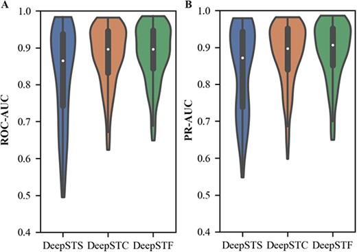
The DeepSTF and variant models' ROC-AUC and PR-AUC distributions.
(ii) This study compares the performance of the model using a multi-headed attention mechanism (DeepSTF) with that using a channel attention mechanism (named DeepSTC) to understand better the advantages of multi-headed attention mechanisms in the model. The channel attention approach is rigorously optimized to reach the greatest outcomes and is then compared with the model provided in the article. Figure 2 shows that both data distributions are identical, indicating that both models have excellent stability. Table 3 shows that, although DeepSTC achieves good performance, it is 1.6%, 0.5%, and 0.8% lower in ACC, ROC-AUC and PR-AUC, respectively, than DeepSTF. Since channel attention concentrates on global information rather than local features and lacks multi-level extraction of shape data, resulting in a considerable drop in model effectiveness. The multi-headed attention mechanism, on the other hand, is capable of capturing different ranges of dependencies within the input sequence, focusing on learning more critical and complex features, paying attention to global information while valuing local features, significantly reducing information loss and achieving a high-level representation of the sequence learned in different representation subspaces. It can be demonstrated that the multi-headed attention mechanism is critical to the model’s performance enhancement, which considerably improves the model’s capacity for acquiring DNA shape features and is more suitable for the proposed DeepSTF model.
The effect of DNA shape on TFBSs identification
We expand the DeepSTF model with three sets of experiments to better understand the function of DNA shape information in predicting TFBSs. First, this research builds a succession of model structures by altering the number of convolutional kernels to evaluate the effect of model complexity on the capacity to capture sequence and shape features. The ROC-AUC changes of the model versions using 32, 64, and 128 convolutional kernels in the motif discovery task are evaluated for each experiment. The impact of various convolutional kernel sizes on the ROC-AUC of this model is shown in Figure 3. The findings from experiments indicate that the model with 32 convolutional kernels has the worst performance, the model with 64 convolutional kernels has slightly better performance, and the model with 128 convolutional kernels further enhances the neural network’s perceptual field and has the best performance. By increasing the number of convolutional kernels to 128, our model can extract higher-order features in the DNA sequence more extensively and better capture the crucial information offered by the DNA shape profile. As a result, the 128 convolutional kernel model is employed for all of the studies.
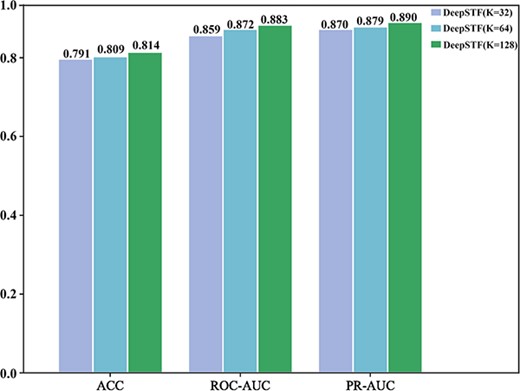
The effect of different convolutional kernel sizes on the DeepSTF model's average ACC, ROC-AUC, and PR-AUC. The value k denotes the number of convolutional kernels, the evaluation metric is represented by the x-axis, and the score is represented by the y-axis. Purple represents the performance of the 32 convolutional kernel DeepSTF model, blue represents the performance of the 64 convolutional kernel DeepSTF model, and green represents the performance of the 128 convolutional kernel DeepSTF model.
After that, we develop DeepSST, a model that takes solely independent DNA sequences as input. The comparative results of the ROC-AUC and PR-AUC of DeepSTF (using sequence and shape as data input) and DeepSST (using only sequence as data input) on a test set of 165 ChIP-seq datasets are shown in Figure 4. It is easy to see that DeepSTF performs significantly better than DeepSST on most of the test sets. This suggests that shape data positively contribute to the vast majority of TFBSs identification tasks and that DNA shape information is critical in the vast majority of TFBSs recognition tasks for the vast majority of cells. Yet, in a few TFBSs recognition tasks, shape information is detrimental to TFBSs prediction, and Supplementary Table S11 details the cell lines of these datasets and the corresponding source organism information. This strongly suggests that the binding mechanism of TFs may differ in different cells, and in some cells, most structural information can be obtained from raw sequence data by stacking convoluted layers and that these cells do not rely solely on DNA shape data, which also implies that the binding mechanism of some TFs is specific to sequence or influenced by other factors rather than shape. Overall, the ROC-AUC and PR-AUC of the DeepSTF improved significantly, demonstrating that for most TFBSs prediction tasks, the average positive contribution of the five shapes information is greater than the average negative contribution, and the addition of shape information improves the prediction accuracy rate of TFBSs.
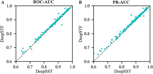
(A) ROC-AUC and PR-AUC comparison of DeepSTF and DeepSST on the test set of 165 ChIP-seq datasets.
Finally, to further explore the contribution of each shape feature to the prediction of TFBSs, we selected the Sknshra P300 ChIP-seq dataset to investigate the effect of each DNA shape information on model performance when predicting P300 TFBSs. The P300 transcription factor interacts with other transcription factors and coactivator proteins to promote gene transcription, and it affects cell development and tissue formation by regulating the expression of key genes. Furthermore, it is involved in regulating the expression of tumor-related genes, which has an impact on tumor biological processes such as cell proliferation, metastasis, and apoptosis. An in-depth study of the functions and regulatory mechanisms of P300 transcription factors can help reveal the molecular mechanisms of disease development and provide new ideas and strategies for the treatment of related diseases. We performed a sensitivity analysis of the DeepSTF model to observe changes in the performance of the predicted P300 TFBSs model by cutting one of the shape information in the input data using the remaining four shape information for the experiment. On this dataset, our model achieves a PR-AUC of 0.866 when all shapes are considered together. Figure 5 shows the overall contribution of Roll, HelT, MGW, ProT, and EP in the prediction of P300 TBFSs. It is easily observed that each DNA shape plays a positive role in the prediction results, with the best performance of the model using a combination of five shapes. The prediction results without considering inter-base pair shapes (Roll and HelT) were slightly lower than those of the five shape combinations, indicating that inter-base pair shapes played a slightly positive role in the predictive power. In contrast, considering the intra-base pair shapes (EP, MGW, and ProT) played a great positive role in the predictive power. EP, MGW, and ProT may be complementary to each other, and the inclusion of these shape information helps to greatly improve the predictive power of the model. This further validates that the inclusion of the five DNA shape features can effectively improve the performance of the model.
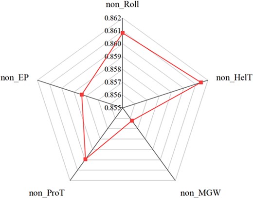
Contribution of Roll, HelT, MGW, ProT, and EP to the prediction of P300 TBFSs.
Cross-cell line TFBSs prediction
To validate the efficacy of the proposed DeepSTF model in learning the general patterns of a specific TF and to increase the model’s generalization and robustness, we construct the model across different cell lines to predict TFBSs in target cell lines. We use ChIP-seq datasets from Helas3, Hepg2, GM12878, and K562 cells in this investigation. Biological experiments demonstrated that the majority of TFs in these cells overlapped. We evaluate the model’s performance using the average ROC-AUC predicted across cell lines. First, we build the DeppSTF model in different cell lines for a specific TF and then utilize it to forecast TFBSs in the target cell line. Figure 6 shows the results of the ROC-AUC comparison between TFBSs cross-cell line prediction and conventional prediction. The average ROC-AUC of cross-cell line prediction is greater than 0.8, demonstrating that our model can effectively predict the location of TFBSs in distinct cell lines. Traditional non-cross-cell line predictions outperformed cross-cell line predictions in the majority of datasets. This result shows that cell line-specific factors are more important in TFs-DNA identification than cell line-independent factors. Cell line-specific factors interact with other cell-specific proteins and co-regulatory factors to ensure accurate gene expression. Therefore, we still need to focus on the role of cell line-specific factors when we delve into the prediction of TFBSs.
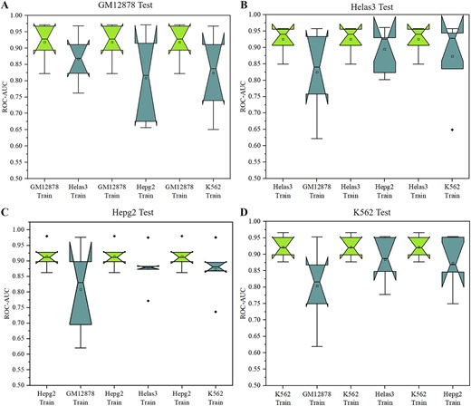
The ROC-AUC comparison between TFBSs cross-cell line prediction and traditional prediction. Cross-cell line prediction indicates that DeepSTF is trained on other cell lines and then used to predict TFBSs in the cell line of interest. (A) Training the model with different datasets and testing it with the GM12878 dataset. (B) Training the model with different datasets and testing it with the Helas3 dataset. (C) Training the model with different datasets and testing it with the Hepg2 dataset. (D) Training the model with different datasets and testing it with the K562 dataset.
Interpretability of the model structure
To better understand what the model learns and how it produces predictions, we use the Hepg2 FOSL2 ChIP-seq dataset to train and test the model’s performance, and we visualize the weights of certain modules in the trained model and the average of the weights to investigate how these modules affect the decision outcome.
The Hepg2 FOSL2 ChIP-seq dataset is a collection of genomic regions bound by the FOSL2 TF in human hepatocellular carcinoma cells (Hepg2 cell line) and is used to explore the FOSL2 TFBSs in the Hepg2 cell line. It contains information on the coordinates of a series of genomic regions identified in the Hepg2 cell line utilizing physical experimental approaches that bind to the FOSL2 TF. These coordinates are typically represented as peak files, with each peak representing a TFBSs. FOSL2 is found on human chromosome 2q33-q34. FOSL2 has a typical binding sequence of 5′-TGAG/CTCA-3′. FOSL2 is involved in a variety of biological processes, including cell proliferation, apoptosis, differentiation, and cell cycle regulation. Furthermore, FOSL2 plays a significant role in the formation and progression of different tumors, including breast, liver, and lung cancers. As a result, investigating the transcriptional regulatory mechanisms of FOSL2 and finding its binding sites is critical for understanding these biological processes as well as studying the occurrence and development of associated disorders.
Figure 7 shows a visualization of the weights of some modules of the DeepSTF model on this dataset, which aids in understanding which features or regions the model concentrates on during the prediction process. The color changes in the figure indicate the relative importance of the associated feature mapping in the model. Lighter colors represent lower values and darker colors represent higher importance. Higher weight values indicate that the model pays more attention to the location, implying that the location is associated with the binding of FOSL2 transcription factors or plays an important role in the prediction of the task. The first eight rows of Figure 7(A) show the weights of each attention head of the multi-headed attention mechanism in the TF module. A darker color represents a higher weight value, indicating that the model pays more attention to that location. Each attention head focuses on different positions, indicating that the model uses different attention points in learning different aspects of TFBSs. As different TFs have varied binding specificities and order preferences, capturing the various properties of these TFBSs can be improved by using multiple attention heads. Furthermore, the variable attentional head focus on different positions indicates changes in the significance and feature contribution of TFBSs. A feature contributes heavily to the prediction of TFBSs in some sequences, while the contribution in other sequences is likely to be relatively small. To better capture these binding sites and improve prediction accuracy, the model needs to employ different attention heads to focus on multiple features at different locations in the input sequence, and multiple heads can capture more comprehensive feature information. The ninth row shows the model’s eight attention heads’ average attention weights. The dark-toned locations highlighted in red are relatively essential in the prediction of TFBSs, which may contain the main features of TFBSs, such as some highly conserved nucleotide sequences. As these characteristics have a greater impact on TFBSs prediction, the model will pay more attention to this location. In addition, the lighter shades at certain locations may be due to average features at these locations contributing less to the model or containing only minor features, such as changes due to certain base variants. The first two rows of Figure 7(B) show the weights of the model’s sequence clade output layer and shape clade output layer. The DNA sequence clade represents a specific base sequence or sequence pattern, whereas the DNA shape clade represents DNA shape features such as tilt and helix angles. It can be seen that the model learns different DNA sequence and shape features in these two clades, and although these features contribute slightly differently to the model, they play a unique role in both clades. The third row shows the enrichment of ChIP-seq signal base pairs for the typical binding sequence 5′-TGAC(G)TCA-3′ of FOSL2. The final row shows the weight visualization results of the model’s final output layer. The output layer concentrates on the middle and posterior feature regions, and the feature regions indicated by the red boxes contribute comparatively more to the model prediction. Consistent with the typical binding sequence of FOSL2, the variation of color tones at critical sites in the weight plot indicates the model responds significantly better to most peaks than to non-peaks, demonstrating the model’s effectiveness in predicting TF-DNA binding events. At the same time, the color of certain positions is slightly lower than adjacent positions, mainly because certain bases are differentially conserved (indicated by the height of the letters in the plot).
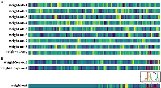
The weight visualization map of certain modules of the DeepSTF model. The color shift at various positions indicates the level of importance, with darker hues signifying more attention. The red boxes indicate portions that are similar to known transcription factor binding sequences. (A) The first eight rows represent the weight maps obtained for each head (eight heads altogether) of the multi-headed attention mechanism in the DeepSTF model. The ninth row represents the average attention weight map of the eight heads. (B) The first and second rows show the sequence clade output weight map and the shape clade output weight map, respectively. The third row shows the enrichment of ChIP-seq signal base pairs for the typical binding sequence 5′-TGAC(G)TCA-3′ of FOSL2, and the fourth shows the model's final output weight map.
To validate the structural similarity of TFBSs predicted by our model to known TF–DNA complexes, we select the Hepg2 CTCF ChIP-seq dataset to investigate the binding pattern of CTCF in HepG2 cell lines. This helps us to investigate the aberrant regulation of CTCF in hepatocellular carcinoma and possible therapeutic targets. To compare the similarity of our model predictions with the structure of the actual TF–DNA complex, we selected the TF–DNA complex associated with the CTCF transcription factor with PDB ID 5YEG in the PDB database. Figure 8 shows the information on TFBSs predicted by our model in the TF–DNA complex and the regional information of the corresponding transcription factors in the TF–DNA complex. The green region indicates the region of TFBSs predicted by our model, which matches the actual complex structure. The colored regions represent the composition of amino acids of transcription factors interacting with TFBSs. By correctly predicting the sequence regions, it is demonstrated that our method shows good performance in predicting TFBSs with better continuity and accuracy. This provides a powerful tool for us to deeply investigate the function and regulatory mechanism of transcription factors and also provides important clues for the study of potential targets in liver cancer therapy.
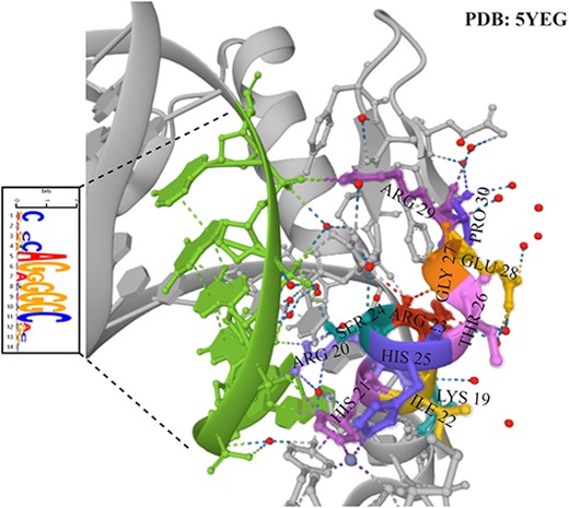
Our model predicts the information of TFBSs in the TF-DNA complex and the regional information of the corresponding transcription factors in the TF-DNA complex. The PDB ID of the TF-DNA complex is 5YEG.The green region indicates the region of TFBSs predicted by our model, which matches the actual complex structure. The colored regions represent the composition of amino acids of transcription factors interacting with TFBSs.
Comparing DeepSTF with existing predictors
To further demonstrate the superiority of DeepSTF, we compare it to DeepBind [30], DanQ [35], DLBSS [20], CRPTS [21] and D-SSCA [22]. To verify the completeness of the experiments and to objectively evaluate the performance of the models, DeepSTF and comparative models are utilized with the 165 ChIP-seq datasets used in Zhang et al. [22]. This study calculates the average ACC, ROC-AUC, and PR-AUC on the test set of 165 ChIP-seq datasets to obtain each model’s final performance. The detailed results are shown in Table 4. Specifically, DeepSTF’s average ACC, ROC-AUC, and PR-AUC scores are 0.814, 0.883 and 0.890, respectively, which are 2.1%, 1.6%, and 1.9% higher than the next best model D-SSCA (0.793, 0.867 and 0.871, respectively). DeepSTF performs well primarily because the model not only fully utilizes CNN to extract higher-order features from sequences but also considers the significance of shape information. It not only uses the residual structure to combine the deep fine information of shape features with the shallow apparent information, but it also employs the multi-headed attention mechanism and the Bi-LSTM operation to adaptively refine the higher-order features derived from the shape information and fully exploit the DNA shape information. The ACC, ROC-AUC, and PR-AUC results of the DeepSTF model are visualized with all comparison models on the test set of 165 ChIP-seq datasets, as shown in Figure 9. DeepSTF outperforms all competing approaches in terms of average ACC, ROC-AUC, and PR-AUC in terms of maximum and minimum values, and it has excellent stability. Furthermore, models that simply use CNN and Bi-LSTM (DeepBind, DanQ, DLBSS, and CRPTS) perform significantly worse than models that include added attention mechanisms (D-SSCA and DeepSTF). This is primarily due to the limited window in the input sequence, and the narrower sequence can just learn the local information of the motif. Adding an attention mechanism can assist the model focus on critical underlying features while suppressing worthless features and learning more extensive and sophisticated relevant features. Furthermore, models that combine sequence with shape for TFBSs prediction (DLBSS, CRPTS, D-SSCA, and DeepSTF) consistently outperform those that use solely DNA sequence features for TFBSs prediction (DeepBind and DanQ). This reveals that the three-dimensional structure of DNA is critical in defining the DNA binding preferences of TFs and other DNA binding proteins. The enhanced prediction performance could be attributed to the fact that most TFs bind to the correct genomic locations via interactions between base-pair readout and shape readout. This implies combining sequence and shape information can increase the model’s prediction power.
The average ACC, ROC-AUC, PR-AUC of DeepSTF model and several advanced methods on 165 ChIP-seq dataset test sets
| Method | ACC | ROC-AUC | PR-AUC |
|---|---|---|---|
| DeepBind | 0.785 | 0.853 | 0.858 |
| DanQ | 0.782 | 0.849 | 0.855 |
| DLBSS | 0.793 | 0.865 | 0.871 |
| CRPTS | 0.793 | 0.862 | 0.867 |
| D-SSCA | 0.793 | 0.867 | 0.871 |
| DeepSTF | 0.814 | 0.883 | 0.890 |
| Method | ACC | ROC-AUC | PR-AUC |
|---|---|---|---|
| DeepBind | 0.785 | 0.853 | 0.858 |
| DanQ | 0.782 | 0.849 | 0.855 |
| DLBSS | 0.793 | 0.865 | 0.871 |
| CRPTS | 0.793 | 0.862 | 0.867 |
| D-SSCA | 0.793 | 0.867 | 0.871 |
| DeepSTF | 0.814 | 0.883 | 0.890 |
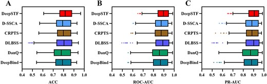
DeepSTF's ACC, ROC-AUC, and PR-AUC were compared with five state-of-the-art methods on a test set of 165 ChIP-seq datasets.
CONCLUSION
We propose DeepSTF, a unique deep learning architecture that combines sequence and shape prediction TFBSs. DeepSTF stacks improved CNNs’ ability to extract high-order DNA sequence characteristics. Meanwhile, the improved transformer encoder structure, CNN, and Bi-LSTM are employed combined to capture higher-order features of shape efficiently. Lastly, the sequence and shape information are merged in the channel dimension for TFBSs prediction. In addition, we explain the utility of the transformer encoder structure and the combined strategy using sequence and shape to capturing multiple dependencies and learning important features. Several experiments on 165 ENCODE ChIP-seq datasets show that DeepSTF performs exceptionally well predicting TFBSs.
Although DeepSTF has numerous advantages, it does have certain limits. First, various factors influence the specificity of TFs-DNA binding, including chromatin structure [36], chemical modifications [37], and nucleosome occupancy [38]. TFs-DNA binding cannot be explained solely by sequence and shape factors [39]. Hence, we intend to investigate other factors in the future. Furthermore, DeepSTF is a network structure for predicting DNA–protein interactions that can be further investigated for application to other bioinformatics prediction challenges, such as predicting DNA–protein binding sites [40–42] and RNA binding sites [43, 44] from protein sequences, thus helping to understand gene regulatory processes at the nucleotide level.
DeepSTF is an approach for transcription factor binding sites (TFBSs) prediction using convolutional neural network, improved transformer encoder structure, and bidirectional long short-term memory, combined with DNA sequence and shape. Benchmarking experiments reveal that DeepSTF beats several state-of-the-art predictors in predicting TFBSs.
We explain the utility of DNA sequence and shape in capturing many dependencies and focusing on learning important features, respectively.
This is the first application of the improved transformer encoder structure to TFBSs prediction, in which the multi-headed attention mechanism enables learning a more comprehensive high-level representation of input information in a different representation subspace, and the module is explained.
The role of different attention mechanisms in the prediction of TFBSs is discussed, and the importance of shape information in the prediction of TFBSs is analyzed.
FUNDING
National Natural Science Foundation of China (62172248); Natural Science Foundation of Shandong Province of China (ZR2021MF098).
Author Biographies
Pengju Ding is a master student at the Qingdao University of Science and Technology, China. Her research interests are bioinformatics and deep learning.
Yifei Wang is a master student at the Qingdao University of Science and Technology, China. Her research interests are bioinformatics and deep learning.
Xinyu Zhang is a master student at the Qingdao University of Science and Technology, China. Her research interests are bioinformatics and deep learning.
Xin Gao is a professor at the King Abdullah University of Science and Technology (KAUST), Saudi Arabia. His research interests include bioinformatics, computational biology, artificial intelligence and machine learning.
Guozhu Liu is a professor at the Qingdao University of Science and Technology, China. His research interests include artificial intelligence, machine learning and algorithms.
Bin Yu is a professor at the Qingdao University of Science and Technology, China. His research interests include bioinformatics, artificial intelligence and biomedical image processing.
