


Abstract
RNAs can interact with other molecules in their environment, such as ions, proteins or other RNAs, to form complexes with important biological roles. The prediction of the structure of these complexes is therefore an important issue and a difficult task. We are interested in RNA complexes composed of several (more than two) interacting RNAs. We show how available knowledge on the considered RNAs can help predict their secondary structure. We propose an interactive tool for the prediction of RNA complexes, called C-RCPRed, that considers user knowledge and probing data (which can be generated experimentally or artificially). C-RCPred is based on a multi-objective optimization algorithm. Through an extensive benchmarking procedure, which includes state-of-the-art methods, we show the efficiency of the multi-objective approach and the positive impact of considering user knowledge and probing data on the prediction results. C-RCPred is freely available as an open-source program and web server on the EvryRNA website (https://evryrna.ibisc.univ-evry.fr).
INTRODUCTION
RNAs can bind and form complexes that have important catalytic functions. One can cite, for example, the ribosome, composed of 5S, 5.8S, 18S and 28S RNAs in eukaryotes, whose role is the translation of messenger RNAs into proteins. The ribosome is also made up of proteins, but it is the RNAs that are responsible for the catalytic activity of the complex. There are also RNA-only complexes, such as the cyclic hexamer of bacteriophage |$\varphi $| 29, used to infect bacteria [1].
RNA complexes can adopt secondary and tertiary structures, expressing their biological function. The prediction of their structure is therefore an important issue, as for RNAs alone. In this study, we address the secondary structure prediction issue. Currently, many bioinformatics tools are available for RNA secondary structure prediction (prediction of the structure of an RNA as in [2–4]), as well as for RNA–RNA interaction (interaction between two RNAs as in [4–6], sometimes including the global structure [5]). But very few tools exist for predicting the structure of complexes composed of more than two RNAs: Table 1 summarizes the existing methods. Note that among these methods, some predict pseudoknots, important motifs in RNA secondary structures, and some are able to return several solutions (an important feature, as RNA complexes can adopt different structures due to the flexibility of RNA molecules).
Biologists have sometimes knowledge that can help the prediction. It can be sporadic information on the structure: pairings, particular motifs, etc. They may also have their own experimental data like SHAPE data [17–19], which give probing information on the considered RNAs. The integration of user knowledge and probing data into the prediction of secondary structures has been used for RNAs alone [18, 20], as well as for RNA–RNA interaction [21]. However, to the best of our knowledge, it is not the case for RNA complexes: none of the methods presented in Table 1 allows the integration of user constraints or probing data.
Summary of the existing methods and tools for the prediction of the secondary structures of RNA complexes composed of several RNAs (more than two). We mention each method’s ability to return several solutions and predict pseudoknots. The tools in gray (NanoFolder and HyperFold) are no longer available or are not usable. No tools are available for [11] and [10] methods.
Summary of the existing methods and tools for the prediction of the secondary structures of RNA complexes composed of several RNAs (more than two). We mention each method’s ability to return several solutions and predict pseudoknots. The tools in gray (NanoFolder and HyperFold) are no longer available or are not usable. No tools are available for [11] and [10] methods.
In this paper we propose C-RCPred, a new method for predicting (in an interactive way) secondary structures of RNA complexes, which allows to integrate probing data and user knowledge. C-RCPred is based on our previously developed method RCPred [14]. RCPred is a method that allows the prediction of (several) secondary structures of RNA complexes including pseudoknots (see Table 1). It takes as input a set of secondary structures per RNA sequence and a set of RNA–RNA interactions per pair of RNAs, which are predicted by existing tools (or provided by the user), and aims to find the best combinations of these inputs, i.e. the combinations leading to complexes with the smallest free energies. For this purpose, it solves a mono-objective graph optimization problem, the clique problem, where the objective function corresponds to the Minimum Free Energy. C-RCPred, the method we propose, is multi-objective. The two new objectives correspond to the agreement with user constraints and the agreement with probing data. The idea is to generate a Pareto set, i.e. a set of RNA complexes structures optimizing simultaneously the different objectives. This leads to a multi-objective version of the clique problem on a weighted graph (with three weights on each vertex). Since it is a generalization of the mono-objective clique problem which is already NP-hard [22], we propose a heuristic based on an adaptation of the Breakout Local Search meta-heuristic [23] to return an approximate Pareto set.
To summarize, C-RCPred takes secondary structures and interactions as input, predicted by existing tools (or provided by the user), as well as user constraints and/or probing data. From these inputs, C-RCPred predicts a set of complexes meeting the different objectives. The structures of these complexes are visualized due to a dynamic graphical interface, from which the user can add new constraints. C-RCPred can then be rerun with these constraints to obtain improved predictions. This cycle can be repeated as many times as needed by the user. Figure 1 gives an overview of our method.
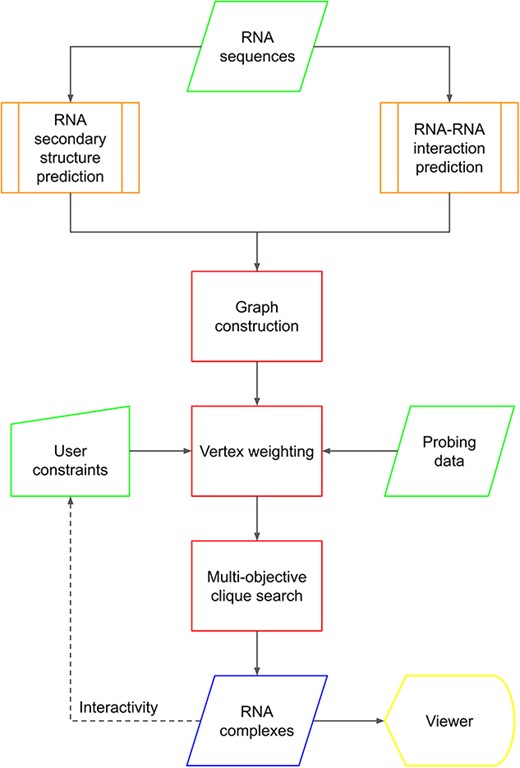
Flowchart describing the C-RCPred method. Input data are represented in green. The predictions of RNA secondary structures and RNA–RNA interactions (in orange) are computed by external bioinformatics tools. The three main steps of the algorithm are represented in red. Output predicted RNA complexes can be visualized and then recalculated if needed using new user-defined constraints.
METHODS
We first present in this section the multi-objective optimization problem to find combinations of structures and interactions corresponding to RNA complexes. Then we describe how we use and implement the new objectives of probing data and user constraints. Finally, we present the multi-objective heuristic we propose to generate an approximate Pareto set for this problem.
The multi-objective clique problem
As stated above, our method is based on a multi-objective graph optimization problem, the multi-objective clique problem, where the following three objectives are considered:
The minimum free energy (MFE) (to be minimized),
the agreement with user constraints (to be maximized),
and the agreement with probing data (to be maximized).
Formally, we define a graph |$G(V,E)$|:
|$V$| is the set of vertices representing the input secondary structures and interactions. A vertex |$v \in V$| corresponds either to a secondary structure or an interaction, and has three weights representing the three objectives given above. The calculation of the weight for the free energy for each input secondary structure or interaction is carried out by the ViennaRNA library [4] with the Turner model [24]. The calculation of the weight for the agreement with user constraints and the weight for the probing data are detailed in the following sections.
|$E$| is the set of edges representing compatibilities between vertices. An edge exists between two vertices if and only if these two vertices are compatible, i.e. when they represent structures or interactions that can belong to the same complex, meaning that no nucleotide is involved in different pairings. If two vertices represent secondary structures of the same RNA, there is no edge between them.
A clique of a graph is a subset of its vertices such that every two distinct vertices in the clique are adjacent (i.e. its induced subgraph is complete). By construction of the graph |$G(V,E)$|, each clique in this graph corresponds to a possible complex. It should be noted that several cliques can correspond to the same complex when the interaction represented by a single vertex is the same as the union of interactions represented by several vertices. Each weight of a clique is calculated by summing the corresponding weights of its vertices. See Figure 2 for an illustration.

Illustration of the multi-objective clique problem in C-RCPred. The square and circle vertices correspond to the secondary structures and the interactions, respectively. There is an edge between two vertices when they represent structures or interactions that can both belong to a valid complex. Each vertex has three weights: the free energy (red), a score related to the agreement with user constraint (green) and a score related to the agreement with probing data (blue). The clique |$c1 = \{i1,i2,s2,s3\}$| (in orange) has a weight of (-14.8, 235, 3.15) and belongs to the Pareto set along with the clique |$c2 = \{i3,i5,s1\}$| (in red) of weight (-15.2, 130.5, 2.1). All the other cliques are dominated by either c1 or c2. For example the clique |$c3 = \{i1,s1,s2\}$| of weight (-13.2, 220, 2.3) is dominated by |$c1$|.
Since we are in a multi-objective context, we search for a set of cliques forming the best possible trade-off, the so-called Pareto set, i.e. cliques minimizing the free energy and maximizing the agreement with user constraints and the agreement with probing data.
User constraints
User constraints are indications of the positions of pairings, non-paired nucleotides or motifs on the complex structure. The possible motifs are helices, pseudoknots, RNA–RNA pseudoknots, terminal loops, internal loops, multi-junction loops (see Figure 8 in Supplementary File). The user can indicate the presence of a motif with (or without) specifying its position and/or the length of the concerned nucleotides.
Each constraint is associated with a confidence index between 0 and 100 (the higher the value, the higher the degree of confidence), which allows the user to weight its knowledge. The confidence index |$IC$| of a structure (or interaction) is calculated as |$ \sum _{i} IC_{i} $| with |$IC_{i}$| the confidence index of a constraint |$i$| satisfied by the structure (or interaction). The user constraint objective corresponds to this confidence index |$IC$|.
Probing data
Probing data are data obtained by experimental techniques yielding an RNA reactivity profile with respect to a chemical or enzymatic treatment. This provides a measure of the likelihood of nucleotides being unpaired or base-paired. More precisely, it corresponds to the reactivity (generally normalized between |$ 0 $| and |$2$|) for each nucleotide. When the reactivity tends toward |$0$|, it means that the nucleotide is probably paired (by a Watson–Crick or G-U pairing), and when it tends toward |$2$|, it means that the nucleotide is probably unpaired. The most known experimental method for getting probing data is SHAPE [17–19]. In order to assess the quality of those data with respect to the reference complex structure, a score must be defined. We use the |$F1$|-score measure:
where |$ TP $| is the number of true positives [nucleotides with a normalized reactivity below a given threshold |$th$| (see Shaker parameters in Results section) and involved in a pairing in the reference complex structure], |$ FP $| the number of false positives (nucleotides with a normalized reactivity below the threshold and not involved in pairing in the reference complex structure) and |$ FN $| the number of false negatives (nucleotides with a normalized reactivity above the threshold and involved in a pairing in the reference complex structure).
Since the experiments carried out for each RNA may be different, a data normalization step is necessary before calculating the score. In the case of SHAPE, the data undergo linear normalization so that the values are between |$ 0 $| and |$1$| [19]:
where |$ r(i) $| is the raw reactivity of the nucleotide |$ i $| and |$ r $| the vector of all the reactivities of the RNA.
Multi-objective heuristic for clique search
The (mono-objective) clique problem is NP-hard [22], and even finding an approximate solution with a performance guarantee for the non-weighted version is hard [25]. As the multi-objective clique problem we consider here is more difficult, the use of heuristics for the resolution of our optimization problem is necessary. In our previously developed method RCPred [14], we used the Breakout Local Search (BLS) meta-heuristic [23] to find good solutions for the mono-objective clique problem. BLS is a recent meta-heuristic that has been successfully applied on several classical optimization problems. In a local search algorithm, one starts from an initial solution and gradually improves it by applying local changes to it. When the solution cannot be improved anymore one gets a so-called local optimal solution. BLS adds a dedicated and adaptive perturbation mechanism to escape local optimal solutions. For a complete description of the BLS heuristic, the reader is referred to the seminal paper [23]. We describe below the modifications applied to make this heuristic multi-objective: the choice of movements in the neighborhood and generation of the Pareto set. Then, we present two modifications to improve the heuristic: generation of the initial clique and condition for stopping the search.
Choice of movements in the neighborhood: In the BLS heuristic, the movement ( i.e. adding a vertex to the current clique, or replacing a vertex in the clique with one that is not in the clique) improving the most the current solution is chosen according to the difference in the scalar weight. In our multi-objective heuristic, we have a weight vector; therefore, we look for a movement whose resulting solution dominates the current one. The local search phase goes on until it is no longer possible to improve the current solution.
Pareto set: Initially the computed Pareto set |$P$| is empty. Then, at the end of the local search phase, we compare the solution |$s$| found with |$P$|. If |$s$| dominates at least one solution in |$P$| or is not comparable with all the solutions in |$P$|, it is added to |$P$|. Solutions of |$P$| that become dominated by the addition of this new solution |$s$| are removed from |$P$|. Then a perturbation is performed on |$s$|, either by starting from a new initial solution |$s^{\prime}$| using vertices not in the previously found clique, or by allowing the removal of a vertex in the clique to escape from the local optimum, and a new local search phase is executed starting from |$s^{\prime}$|.
Generation of the initial clique: In the BLS heuristic, this procedure consists of randomly selecting a vertex and then iteratively adding to it vertices that can form a clique, until there are no more vertices that can be added. In our algorithm, this procedure randomly selects a single vertex constituting a clique. The clique will then grow due to the local search phase.
Heuristic stop condition: In the BLS heuristic, the stop condition occurs either when the exact solution is found (if this information is available), or when a maximum number of iterations is reached. In our algorithm, we choose to stop the search when either a maximum number of iterations is reached or when we notice that the search is stagnating, or in other words, the search remains blocked in a local optimum, despite two random perturbations of the solution.
It should be noted that the neighborhood has a polynomial size with respect to the number of vertices of the graph. However, the number of iterations, and thus the overall complexity, depends on the stop condition chosen. Experimental running times are reported in Running time section in Supplementary File, Figure 10.
RESULTS AND DISCUSSION
Benchmark datasets and measures
Using available public databases (RNA STRAND [26] and RNAsolo [27]), we were able to get 108 RNA complexes to evaluate C-RCPred (see Supplementary File for details on the dataset construction). The complexes in this dataset have lengths varying between 24 and 968 nt, each composed of 3 to 8 RNAs of different lengths (2 to 247 nt). Among these complexes, 20 contain pseudoknots.
For our benchmarks, we used the Matthews correlation coefficient (MCC) introduced in [28] and commonly used in RNA secondary structure prediction [29] (see Supplementary File for the formula). As stated in the Introduction, RNA complexes can adopt different structures. Our method returns several solutions corresponding to possible secondary structures of complexes composed of the RNAs given in input. However, in our benchmark dataset, only one reference structure is available for each complex. Therefore, to evaluate the performance of C-RCPred, we determine if, among the returned solutions, one is close to the reference structure. In the following text, we thus show the results corresponding to the solutions with maximum MCC. In the experimentations given in the sequel of the paper, when we fix the number of returned solutions for C-RCPred or other tools, it should be noted that it is an upper bound on the number of different solutions effectively returned. Indeed, some solutions can be identical, or the tool cannot generate as many solutions. Finally, since a heuristic is used, several executions of the program are performed, and an average of the different maximum MCC (obtained at each execution) is calculated.
Tools used upstream
As mentioned above, tools for predicting each RNA’s secondary structures and interactions between each couple of RNAs are used upstream of C-RCPred. Many tools exist in the literature, as mentioned in [30]. We chose here to mainly use tools able to return several solutions, since C-RCPred requires several structures and interaction inputs. For secondary structure prediction, we use Biokop [3], pKiss [2] and RNAsubopt [4] that return several solutions, and MXfold2 [31] which returns only one solution. Note that Biokop and pKiss predict pseudoknots, but not RNAsubopt and MXfold2. For RNA–RNA interactions, we use IntaRNA [5], RNAplex [6] and RNAsubopt [4]. Of course, other tools can easily be added, due to the modular implementation of our method.
We chose to predict a maximum of 10 structures per tool, using their default parameters, and we chose to predict a maximum of 30 interactions per tool, with also their default parameters (the justification for choosing these values is given in Supplementary File).
Another tool we integrated into our framework is a tool for probing data prediction, called Shaker [32]. Shaker uses a graph-kernel-based machine learning approach to predict SHAPE values on each nucleotide of a given RNA sequence. The higher the value corresponding to a nucleotide, the lower the probability that the nucleotide is paired, and inversely. After a linear normalization (by C-RCPred), these values are between 0 and 1. Therefore, when a value is close to 0.5, it is not informative. We introduced a threshold value |$th$| varying between 0 and 0.5, such that C-RCPred considers only Shaker values below |$th$| and above |$1-th$|. We consider by default a threshold of 0.3 (see Supplementary File, Figure 3).
Evaluation of our clique problem approach and BLS heuristic
Our approach is based on the assumption that the closer a clique is to the exact Pareto front (which is the image of the Pareto set in the objective space), the higher in average the MCC of the associated complex is. In order to evaluate this assumption, as well as the quality of the proposed heuristic to find multi-objective cliques close to the Pareto front, we have followed an exhaustive approach, when it was computationally possible. More precisely, given a complex, we computed the set of all the cliques in the graph generated by C-RCPred. This has allowed us to retrieve the exact Pareto front. Moreover, we computed the MCC for each complex corresponding to each clique in the graph. We were able to compute all the cliques from the graphs of 61 complexes out of the 108 (see Figure 3, and Figures 5 and 6 in Supplementary File, due to the python package NetworkX (https://networkx.org) [33] and the function clique.enumerate_all_cliques adapted from [34]). Details are given in Supplementary File.
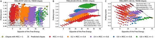
Visualization of all the cliques of the graph constructed by C-RCPred for the complexes PDB_00747 (A), PDB_01126 (B) and PDB_00871 (C). Each dot represents a clique and is colored according to its MCC value. The weight of each clique is composed of two values: on the x-axis the opposite of its free energy and on the y-axis its probing score. The crosses represent the set of all the cliques that C-RCPred returns over 100 executions. The stars represent the cliques with a MCC of 1, that is, the cliques corresponding to the reference complex. The dotted line represents the exact Pareto front. When there are several cliques at the same position (with the same free energy and the same probing score), their average MCC is reported.
For illustration, we show in Figure 3 the generated cliques for three complexes: PDB_00747, PDB_01126 and PDB_00871. The structures and interactions belonging to the reference complex have been added to the set of structures and interactions given as input to C-RCPred. Therefore, each graph has at least one clique corresponding to the reference complex. As we can see, the best solutions, i.e. the ones with a MCC over 0.8 (represented in green), are located in a region quite close to the exact Pareto front (represented with a dashed line). On the contrary, when looking at the worst solutions, i.e. the ones with an MCC below 0.2 (represented in red), most of them are located in regions far away from the exact Pareto front. Moreover, the cliques with a MCC=1 corresponding to the reference complexes (represented by a star) are located either on the exact Pareto front or close to it. These observations are in accordance with our assumption that the majority of the good solutions are close to the exact Pareto front.
The exact Pareto front can contain solutions with a low MCC, as in PDB_01126 and PDB_00871 complexes (Figures 3B and 3C). A possible explanation is the varying role played by the objective functions from one complex to another, and also the quality of the probing data generated by Shaker. For PDB_01126, Shaker generates very good probing data, since the F1-score is close to 0.9 (see Figure 6). We can see that the best solutions are located at the top of the figure, which means that this criterion (probing score) is predominant in determining good solutions, and the energy criterion is less important. On the contrary, for PDB_00747, the probing data are not useful, since their F1-score is close to 0 (see Figure 6), and this time the energy criterion is more relevant. We can observe that the best solutions are located on the right of the figure.
The reference solution can be at an extremity (PDB_00871, Figure 3C) or rather at the top side (PDB_01126, Figure 3B) or right-side (PDB_00747, Figure 3A). That is why we do not favor one region over another in our approach, and prefer to obtain the whole Pareto set.
Finally, we can see that the Pareto front predicted by C-RCPred is of very high quality. Indeed, the set of all the cliques predicted by C-RCPred (represented on the figures by the crosses) are located on the exact Pareto front.
Evaluation of C-RCPred in function of the number of generated complexes
Here we evaluate the impact of the number of returned solutions on the probability of getting, among the predicted structures, the real structure or at least a structure close to the real structure. We can see in Figure 4 that from 20 solutions, both the MCC and the probability of getting a solution with MCC=1 become stable. We therefore choose to set by default the number of returned solutions to 20.
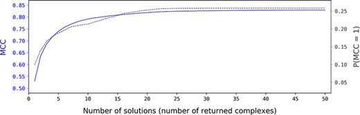
Impact of the number of returned solutions by C-RCPred on its prediction results. For each complex in the dataset, the average value over 100 executions of the maximum MCC of the solutions returned by C-RCPred is computed. Then, the average value of these quantities is computed over all the dataset complexes and is reported in function of the number of returned solutions (blue curve). The average probability (between 0 and 1), over all the dataset and over the 100 executions for each complex, of getting a solution with MCC=1 during an execution (P(MCC) = 1) of C-RCPred is also reported (black curve).
Evaluation of C-RCPRed in function of the input predicted RNA structures and interactions
As explained above, C-RCPred algorithm takes as input a set of RNA structures and RNA–RNA interactions that constitute the graph vertices of our clique optimization problem. Figure 5 gives, for each complex, the best MCC of C-RCPred predictions, along with the best MCC of secondary structure predictions of each RNA and the best MCC of interaction predictions of each couple of RNAs. We can see that in all complexes, some structures and/or interactions are not well predicted (MCC close to zero) by the used tools upstream, and despite this, C-RCPred succeeds in returning good predictions in almost all cases: this appears for instance for complexes involving unstructured RNAs. For the cases where the MCC of C-RCPred is very low, one possible explanation is that the best predicted structure for an RNA has an energy that is not the lowest one, and therefore do not belong to the selected cliques since energy is one of the considered objectives. It is the case, for instance, of PDB_00340, PDB_00370 and PDB_00679, for which the MCC is equal or close to zero.
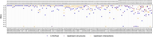
MCC values obtained with C-RCPred, compared with those of the predicted upstream structures and interactions. The maximum MCC of the 20 first returned solutions by C-RCPred for each complex is kept in each execution and the average over 100 executions is reported. The maximum MCC is also kept for the predicted secondary structures for each RNA and for the predicted interactions for each couple of RNAs. In case of nonstructured RNA, the MCC of the upstream predictions is not reported, since it is irrelevant ( Notice that in case of a nonstructured RNA one has always TP=FN=0 in the MCC formula, meaning that the MCC is always equal to 0.). In the top axis, for each complex is given its length and (in parentheses) the number of RNAs composing it.
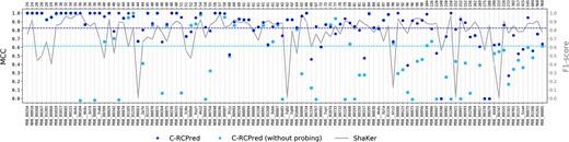
MCC values obtained by C-RCPred with and without the Shaker probing data on our benchmark dataset, sorted by complex length. C-RCPred is run 100 times, and the maximum MCC of the 20 first returned solutions is kept in each run. The dots thus correspond to the average of the 100 obtained maximum MCC. The two dashed lines correspond to the average MCC calculated for the whole dataset. The gray curve gives the F1-score of Shaker predictions.
We performed additional experiments to evaluate the effect of the RNA secondary structures and interactions input on C-RCPred results. We use the ground truth secondary structures and interactions (generated from the dataset complexes) as input. Details of these experiments and the obtained results are provided in Supplementary File (Section ‘Upstream tools’, Figure 2). The overall conclusion is: (i) as expected, C-RCPred successfully predicts the correct complexes from the ground truth inputs; (ii) C-RCPred results would only be marginally affected by the addition of a theoretical and perfectly accurate prediction tool.
Finally, one can wonder if the number of structures and interactions upstream influences the results. Such information are given in Supplementary File, Figure 1.
Evaluation of the probing data objective
Unfortunately, it is very difficult to find probing data for RNAs belonging to complexes of more than two RNAs. To evaluate the probing data objective, we therefore used artificial probing data predicted by the tool Shaker [32] presented above.
Here, we evaluate how the probing data improve the prediction results of C-RCPred. Figure 6 gives the MCC values obtained by C-RCPred, when using or not using probing data. As we can see, C-RCPred produces better results when using probing data. On average, the MCC is increased by 0.2 but, for some complexes, the MCC goes from 0 to 1. This occurs particularly when the F1-score of Shaker is equal or close to 1.
Evaluation of the user constraints objective
To assess the contribution of user constraints as an additional objective, we tested C-RCPred on the PDB_01260 complex from our benchmark dataset. The structure of this complex, composed of three RNAs, is represented in Figure 9A in Supplementary File. This complex, as shown in Figure 9B and 9C of the Supplementary File, is incorrectly predicted, even with the use of probing data.
To assess the effect and interest of using user constraints, we consider one (biologically) valid constraint, corresponding to a true pairing between RNA1 and RNA2 (constraint |$a$|), and two nonvalid constraints, one corresponding to a false pairing in RNA3 (constraint |$b$|) and the other to a false hairpin loop motif in RNA1 (constraint |$c$|). Thus, the constraint |$a$| should improve the prediction results, while |$b$| and |$c$| should degrade them when they are satisfied.
The obtained results are given in Figure 7. We modulated the confidence index between |$ 50 $| and |$ 100 $|. A high confidence index indicates that the user is very confident in this constraint, which is therefore favored in C-RCPred.
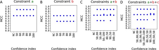
MCC of the predicted structures by C-RCPred of the complex PDB_01260 when considering user constraints. C-RCPred was executed 100 times and the 20 first solutions were kept at each run. Then are reported the MCC of the different obtained solutions (blue dots). The confidence index varies from |$50$| to |$100$|. The constraints used are mentioned in the figure (in green if they are biologically valid, in red if not). The condition ‘NC’ (for ‘No Constraint’) is a control test.
We also reported, as a control, the results of C-RCPred without the use of constraints. As we can see in Figure 7A, adding the constraint |$ a $| increases the quality of the results: the maximum MCC goes from around 0.6 to around 0.9. On the contrary, adding the constraint |$b$| decreases the results, as shown in Figure 7B. The same results are obtained when using the constraint |$c$| (data not shown). Figure 7C gives the results when both |$a$| and |$b$| constraints are used with different confident indices. We can see that when the constraint |$a$| has a lower confidence index than the constraint |$b$|, we have worse solutions than when it is higher. This is even more obvious when we combine the three constraints |$a$|, |$b$| and |$c$| as shown in Figure 7D. Thus, the outcome is as expected: the higher the confidence indices of the valid constraints compared with the ones of the non valid constraints, the better the results.
Finally, as the results show, when constraints are specified by the user, they are respected by our algorithm, taking into account the simultaneous use of several constraints, as well as their different confidence indices. The structures corresponding to the solutions with the best MCC are visualized in Figure 9D, 9E and 9F of the Supplementary File. As we can see, the predicted structure that is the closest to the reference structure is the one predicted when considering constraint |$a$|.
Comparison with the state-of-the-art
We present here the prediction results obtained on our benchmark dataset by C-RCPred, compared with those obtained by other existing tools for predicting the structure of RNA complexes (see Table 1), namely: NUPACK [8], MultiRNAFold [7], RCPred [14], RNAmultifold [15] and VfoldMCPX [16].
C-RCPred is run using SHAPE data generated by Shaker [32] with a threshold equal to 0.3. In this benchmark, no user constraint is used. VfoldMCPX provides the possibility to predict or not the pseudoknots. We use it with the second option since we are interested here by predicting structures integrating pseudoknots. The other tools are run with their default parameters.
We should note that MultiRNAfold and VfoldMCPX were unable to predict solutions for several complexes: VfoldMCPX was unable because the complexes are too long, and the current version of MultiRNAFold in some instances detects nonexistent characters in the input sequence. Therefore when we average MCC values on the whole dataset, we do not count those of four (respectively, 19) complexes for MultiRNAFold (respectively, VfoldMCPX).
Figure 8 presents the MCC obtained by the different tools according to the number of returned solutions. As we can see, from 10 returned solutions, C-RCPred results are much better than those obtained by the other tools. The results of C-RCPred are not so good when only one solution is returned. This is not surprising since our method has been designed to return several solutions. As stated in the Introduction section, RNAs are not stable and can adopt different structural conformations; therefore, predicting only one possible structure is simplistic and limiting [35]. Thus, when C-RCPred returns only one solution, it may be correct without being the reference structure in the considered dataset.
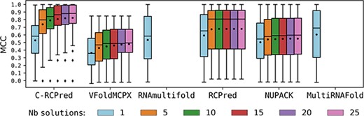
Results obtained by C-RCPred and the other tools of the state-of-the-art on our dataset, in function of the number |$N$| of returned solutions. For each complex, C-RCPred and RCPred are run 100 times. In each run the maximum MCC over the 20 first returned solutions is kept, and the average of these maximum over the 100 executions is computed. Then statistics on those averages are computed over all the dataset complexes.
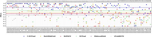
Results obtained by C-RCPred and the other tools of the state-of-art on our dataset. C-RCPred is run 100 times. In each run the maximum MCC over the 20 first returned solutions is kept, and the average of these maximum MCC over the 100 executions is reported for each complex. The horizontal dashed lines correspond to the mean over all the dataset complexes. On the top X-axis is given the size of each complex.
Details of the MCC obtained by each tool for each complex are shown in Figure 9, considering here 20 returned solutions which is our parameter by default. On average for all the dataset, C-RCPred achieves an MCC larger than 0.8, while the MCC of RCPred, MultiRNAFold, NUPACK, RNAmultifold and VfoldMCPX are around 0.69, 0.6, 0.55, 0.54 and 0.5, respectively. From the figure, we can see that C-RCPred has far fewer cases of MCC equal to zero or less than 0.5 compared with the other tools. In particular, C-RCPred has an MCC equal to zero for only three complexes, for which no other tool succeeds.
Comparisons with the state-of-the-art using other measures are provided in the Supplementary File, Figure 7, leading to the same conclusions.
In Figure 10 we illustrate how our method C-RCPred succeeds to predict the secondary structure of a complex, the PDB1FOQ (of length 597 bp), on which the other tools fail. C-RCPred was run in the same condition as above, i.e. using Shaker probing data but without any user constraint. Note that VfoldMCPX was not able to process this complex because of its length. Prediction results (based on different measures) obtained on this complex by the different tools are provided in Supplementary File, Table 1. The MCC of C-RCPred is very high (|$\approx $|0.95). The second best MCC is obtained by RCPred (|$\approx $|0.42) then RNAmultifold (|$\approx $|0.40). RCPred succeeded in returning the structure of one of the five arms of the complex (each arm corresponds to an RNA).
![Secondary structure of the pentameric prohead RNA of the bacteriophage (29 (PDB code 1FOQ): comparison between (A) the reference structure and predictions generated by (B) C-RCPred, (C) RCPred, (D) MultiRNAFold, (E) RNAmultifold and (F) NUPACK. The structures shown correspond to the solutions with the best MCC. The visualizations are rendered with the Ribosketch tool [36].](https://oup.silverchair-cdn.com/oup/backfile/Content_public/Journal/bib/24/4/10.1093_bib_bbad225/1/m_bbad225f10.jpeg?Expires=1750300971&Signature=j8DyjZctL8-rBdRyLyKUK-bA3W4hoSBB6UydIIRFaUgwS9Y74b3eFWp7IgIqShtehdK02dX9YYg-P2lV6KdBz2Ydbw~f-3mD9ylFFmWb~-SROy94ltnxNAWi8w94SnKIYf0s5DJUSBftI1cNX1NHqiAuAk~RkiYGvJ3sXJSdyD57Y3BOiR4ffKbi5hjHvUmtg0RMB07bt8KVIpIs5VT~7SpZola7nq4DhSnLncJ5Tbh~Cu4NtqXJ~POz62x7xZU4waVmqhZwr9keRpqjZz1thCihLsqObIHVCTI2~jkZjsNAc9kXmE3QZg6Lhjtt1b8IT3zFZWlcb9HWCvFs0Y645Q__&Key-Pair-Id=APKAIE5G5CRDK6RD3PGA)
Secondary structure of the pentameric prohead RNA of the bacteriophage (29 (PDB code 1FOQ): comparison between (A) the reference structure and predictions generated by (B) C-RCPred, (C) RCPred, (D) MultiRNAFold, (E) RNAmultifold and (F) NUPACK. The structures shown correspond to the solutions with the best MCC. The visualizations are rendered with the Ribosketch tool [36].
CONCLUSION
We presented in this paper a new method called C-RCPred, for secondary structure prediction of RNA complexes. C-RCPred is based on a multi-objective approach where the objectives are the free energy, user constraints and probing data.
Experimental probing data for some RNAs can be found in databases. However, to our knowledge, there is no specific probing data for RNAs involved in complexes and very few data are available. A recent tool, called Shaker [32], allows to predict SHAPE data for RNAs. We have shown that adding these predicted data in our multi-objective method improves the obtained results. The current version of C-RCPred allows considering one file of probing data as an input. We can consider the possibility of having several probing data coming from different experiments (and/or different predicted probing data). A way to consider all of them would be to aggregate them into one input. However, this leads to bias, and extracting reliable reactivity information from multiple SHAPE replicates is a research area [37]. Another way would be to consider each probing data set as a different input, and then as a different objective due to our multi-objective approach.
Other objectives could be added to our multi-objective method. Besides the MFE model which has been considered here, we can also use the MEA model, as done in BiokoP method [3], where the combination of the two models MFE and MEA has shown an improvement of the results compared with using one model alone. We can also add as an objective the insertion of 3D RNA motifs, as done in BiORSEO method [38].
A future work is to extend our method to consider noncanonical interactions. This implies using upstream tools to predict secondary RNA structures and RNA–RNA interactions with noncanonical pairings.
Another perspective of work would be to add downstream to C-RCPred a module for reducing the number of returned solutions, in order to facilitate user analysis of the results. A possibility would be a clustering module, which will put similar predicted structures into groups, and return a consensus structure for each group.
While many tools exist for the prediction of RNA structures and RNA–RNA interactions, very few tools exist for the prediction of RNA complexes structure.
We propose C-RCPred for the prediction of RNA complexes including pseudoknots, which takes into account user knowledge and probing data and which is able to return several solutions.
C-RCPred is based on a multi-objective optimization algorithm, and the implemented objectives are the global energy of the complex (MFE), the agreement with user constraints and the agreement with probing data.
The performed benchmarks show the efficiency of the multi-objective approach, and the positive impact of considering user knowledge and probing data on the prediction results. They also show C-RCPred gives better prediction results compared with the state-of-the-art methods.
C-RCPred is an interactive tool, freely available on our bioinformatics platform dedicated to RNA and called EvryRNA: http://evryrna.ibisc.univ-evry.fr.
AUTHOR CONTRIBUTIONS STATEMENT
E.A., A.L. and F.T. conceived the algorithms; E.A and F.T conceived the experiments; M.I. conducted the experiments; E.A., M.I. and F.T. analyzed the results; A.L, M.I and G.P. worked on the implementation and the web server; E.A and F.T. supervised the work. E.A. and F.T. wrote and reviewed the manuscript; G.P. reviewed the manuscript.
Author Biographies
Mandy Ibéné holds an MSc in Bioinformatics. She worked during her Master 2 internship on C-RCPred under the supervision of Fariza Tahi and Eric Angel.
Audrey Legendre holds an MSc and a PhD in Bioinformatics. Under the supervision of Fariza Tahi and Eric Angel, she developed multi-objective algorithms for secondary structure prediction of RNAs and RNA complexes.
Guillaume Postic is an assistant professor of Computational Biology at Université Paris-Saclay, Univ. Evry. His research focuses on the 3D structure of RNA macromolecules.
Eric Angel is a full professor of Computer Sciences at Université Paris-Saclay, Univ. Evry. His main research are in multicriteria optimization and algorithmics.
Fariza Tahi is a full professor of Computer Sciences and Bioinformatics at Université Paris-Saclay, Univ. Evry. Her group develops algorithms and tools for the analysis of ncRNAs and the prediction of their 2D and 3D structures.
REFERENCES
