DIST: spatial transcriptomics enhancement using deep learning Free

Abstract

Introduction

Spatial transcriptomics (ST) is a recent technological innovation that enables the measurement of gene expression with spatial information in tissues. Knowledge of the relative locations of transcripts is critical for understanding biological, physiological, and pathological processes, and therefore, ST technologies have been used in various biological fields, such as tumor microenvironment [1, 2], embryonic development [3, 4] and neurology [5, 6]. ST technologies can be primarily classified two categories: (1) next-generation sequencing (NGS)-based approaches, such as ST [7] and 10X Genomics Visium [8], encoding positional information onto transcripts before sequencing and (2) imaging-based approaches, comprising in situ sequencing-based methods, represented by FISSEQ [9] and STARmap [10], in which transcripts are amplified and sequenced in the tissue, and in situ hybridization-based methods, represented by MerFISH [11] and seqFISH [12], in which imaging probes are sequentially hybridized in the tissue [13].

There is generally a trade-off between resolution and gene throughput in these technologies. Imaging-based approaches provide increased resolution and sensitivity, but have lower throughput, limiting their potential to explore transcriptome-wide interactions and discover new sequences. NGS-based methods are unbiased, as they can in principle sample the whole transcriptome, but have lower resolution and sensitivity [13–15]. More recently, the resolution of NGS-based methods has rapidly increased, for instance, DBiT-seq [16] reaches ~10 μm resolution and Stereo-seq [17] achieves nanoscale resolution (220 nm). While these NGS-based methods measure the expression level for thousands of genes in captured locations, referred to as spots, they suffer from incomplete spatial coverage, limiting their usefulness in studying detailed expression patterns. ST has 100 μm spot diameter with 200 μm center-to-center distance and Visium has 55 μm spot diameter with 100 μm center-to-center distance. The theoretical center-to-center distance of DBiT-seq can be as small as 2 μm because of the diffusion distance that is ~1 μm. Standard DNA nanoball chips of Stereo-seq have spots with ~220 nm diameter and a center-to-center distance of 500 or 715 nm.

The diameter and density of measured spots both limit the spatial resolution of current NGS-based methods, ranging from multicellular to subcellular [14]. To get high-resolution (HR) spatial expression profiles, new methods have been developed. For example, BayesSpace [18] employs a Bayesian method that uses the information from spatial neighborhoods for resolution enhancement, but BayesSpace improves the resolution by inferring the expression of sub-spots and cannot predict the expression on unmeasured locations; XFuse [15] uses a deep generative model trained by spatial expression data and corresponding histology images to infer super-resolved expression maps; HisToGene [19] is a deep learning method adopting Vision Transformer for gene expression prediction from histology images; SpatialPCA [20] extracts a low-dimensional representation of normalized and scaled ST data leveraging modified probabilistic principal component (PC) analysis, and can impute spatial PCs on unmeasured spots because of the data generative nature.

However, these existing methods either rely on histology images with obvious texture, or use the original expression information inefficiently. Some only get HR normalized or scaled data and fail to account for the mean-variance relationship existed in raw counts, leading to a potential loss of power [21]. Here, we mainly focus on NGS-based ST techniques with non-dense spatial coverage. Considering that successful applications to ST of deep learning [22–24], the nature connection between gene expression with spatial information and images and inspired by learning-based image processing [25, 26], we propose DIST, a method that imputes gene expression profiles on new and unmeasured spots only using spatial gene expression data to get a refined spatial map with a higher resolution. Unlike XFuse and HisToGene, DIST enhances the ST data using deep learning and does not need any additional information such as the histology image. In addition, despite improvements in NGS-based ST technologies, various technical factors including amplification bias and especially low RNA capture rate lead to substantial noise in sequencing [27]. The challenge is even greater for technologies with relatively HR because of relatively shallow sequencing. Noise because of amplification and dropout events may obstruct analyses and corrupt the underlying biological signals. For solving this problem, DIST can denoise imputed spatial gene expression by learning from high-quality data. Overall, we explain DIST as denoising and imputing spatial transcriptomics. We illustrate the benefits of DIST through simulation from a STARmap data set and a Stereo-seq data set and applying it to two real-world data sets obtained with, respectively, ST and 10X Visium platforms. We show that DIST could accomplish imputation task more accurately than conventional interpolation methods, meanwhile reveal more biological signals.

Methods

Overview of DIST

DIST mainly focuses on array-based ST techniques. Measured spots of these techniques arrange in certain patterns, generally comprising two classes: matrix arrangement such as ST and honeycomb arrangement such as Visium. DIST predicts an unmeasured spot between every two adjacent measured spots (Figure 1A).

Figure 1

The architecture of DIST. (A) Sketch of imputation and down-sampling on the platform having matrix (above) and honeycomb (below) permutation. Impute: predicting a new spot between every two adjacent spots. Down-sample: extracting nonadjacent spots regularly at intervals of one spot. (B) Self-supervised learning framework. Down-sample: down-sampling the original gene expression maps and creating artificial lower resolution gene expression maps to form LR-HR gene expression pairs. Training process: training an interpolation deep neural network, VLN, in a supervised manner using down-sampled LR gene expression as inputs and the original gene expression as labels. Prediction process: feeding the original gene expression maps into the trained model to output higher-resolution gene expression. (C) The network architecture of VLN.

Open in new tabDownload slide

The whole idea of DIST is imputing the gene expression of unmeasured spots by self-supervised learning. Since we do not have low-resolution (LR) and HR gene expression pairs for training, we down-sample the original gene expression maps and create artificial LR gene expression maps to train the model. As shown in Figure 1B and C, DIST first trains an interpolation deep neural network, variation learning network (VLN) [26], in a supervised manner using down-sampled LR gene expression as inputs and the original gene expression as HR labels. The outputs are the imputed gene expression maps with the same resolution as original data. Then in the prediction phase (or imputation phase), the original gene expression of all spots is fed into trained model to output HR gene expression. DIST first learns how to impute the unmeasured gene expression from down-sampled LR gene expression maps and original gene expression maps and then applies the learned rules to impute the unmeasured gene expression on original data. This architecture allows DIST to enhance the ST data by various ways. Besides imputation of unmeasured spots by self-supervised learning, DIST can improve imputation of low-quality ST data by transfer learning on a high-quality ST data and denoise imputed expression by introducing synthetic noises to inputs of training set.

DIST method

DIST finishes imputation only using gene expression matrix with spatial coordinates for any data space, such as gene counts, normalized gene counts and other embeddings. In this paper, we mainly analyzed gene counts matrix.

Mostly, missing values exist when gene expression is transformed to an expression map because of irregular graphics of tissue section and filtering spots with poor quality. These missing values are simply set to 0. We do not consider out-tissue spots where there are no cells at all. Therefore, our method focuses on in-tissue spots and recovers the details inside tissue section.

The shape of |${L}_{\mathrm{train}}^j$|is |$\left(\left[{u}_{\mathrm{train}}/2\right],\left[{v}_{\mathrm{train}}/2\ \right]\right)$|⁠, where |$\left[\cdot \right]$| means the rounding operation.

We use ADAM optimizer to minimize the loss via mini-batch gradient descent.

If |${I}_{\mathrm{train}}$| and |${I}_{\mathrm{test}}$| come from the same ST data, the learning process is self-supervised learning; if not, then it is transfer learning.

The architecture of VLN

As shown in Figure 1C, VLN takes a recurrent convolutional structure that performs a progressive recovery route in a supervised manner [26]. Suppose that there is an HR expression map |$y$| and it is split into four parts: |${x}_{tl}\ \left(=x\right),{x}_{tr},{x}_{bl}$| and |${x}_{br}$|⁠, the sub-maps consisting of the top-left, top-right, bottom-left and bottom-right values extracted from every 2 × 2 nonoverlapping patches. VLN estimates the mapping |$y=F(x)$| to recover HR |$y$| from LR down-sampled |$x$|⁠. We suppose the shape of |$x$| is |$\left(u,v\right)$|⁠.

During the training phase, |$K=2$| and |$L=5$| by default. The learning rate is set to 0.001 for front-end layers and 0.00001 for the reconstruction layer. In most cases, the loss will converge within 200 epochs.

Introduction of synthetic noises

DIST can denoise the imputed expression by introducing synthetic noises to the inputs during the training process. Following SAVER [28], we introduced noises to the gene expression as follows: for gene |$j$|on spot |$i$|⁠, we treated the original count as |${X}_{ij}$|⁠, and the noised value |${Y}_{ij}$| was generated by drawing from a Poisson distribution with |${Y}_{ij}\sim \mathrm{Poisson}\left(\lambda{X}_{ij}\right)$| where |$\lambda$| is efficiency loss. We let |$\lambda =0.6$| for introducing noises to Visium human invasive ductal carcinoma (IDC) data [29] in the subsequent experiment.

Data analysis

We explored biological functions of IDC following the conventional analysis processes including quality control, normalization, clustering, differential expression analysis and pathway enrichment [30]. We used log-transformed normalization, selected 2000 highly variable genes and applied Louvain [31] to cluster spots. Since existing approaches of identifying significant differentially expressed (DE) genes mostly suit for integer unique molecular identifier (UMI) counts, we rounded the imputed counts before differential expression analysis. We used t-test to find DE genes and chose significant DE genes by thresholds of adjusted P-value and log2-foldchange, and these values are listed as follows:

• (i) Comparison between original and imputed IDC: adjusted P-value < 0.05 and log2-foldchange > 1;

• (ii) Comparison between denoised and non-denoised IDC: adjusted P-value < 1×10^-6 and log2-foldchange > 0.6.

Enrichment analysis was accomplished at Metascape [32] website.

Results

DIST imputes the spatial gene expression accurately

To rigorously evaluate the imputation performance of DIST, we created a simulated ST data from a STARmap data set, in which RNA molecules from 903 genes had been measured and located on a mouse placenta tissue [33]. We used this molecular-resolution data to simulate a single-cell-resolution spot-like data by projecting all RNAs onto pseudo spots (240 × 240 pixels). The total RNA counts within a 240 × 240 pixels’ scope were considered as gene expression of this simulated pseudo spot. As a result, there were totally 7465 pseudo spots with more than 5 RNA counts. The number of pseudo spots approximately equals to cells number estimated by ClusterMap [33]. We used this simulated single-cell-resolution data set as ground truth and down-sampled it to create a simulated coarse-resolution ST data. Then we compared DIST with other interpolation methods including nearest neighbor (NN), linear barycentric interpolation (Linear), cubic spline interpolation (Cubic), new edge-directed interpolation (NEDI) [34], fast image interpolation via random forests (FIRF) [35] and SpatialPCA. We did not compare DIST with state of art methods such as BayesSpace, XFuse and HisToGene for ST imputation because BayesSpace separates a spot into several sub-spots and cannot impute gene expression for unmeasured locations; XFuse and HisToGene need histology images that cannot be provided by simulation. Since the number of genes in simulated data is smaller than that of the whole transcriptome by over an order of magnitude, we pretrained DIST with IDC data, and then fine-tuned the model on the training set constructed from the simulated data itself.

Figure 2A and Supplementary Figure S1 show the ground truth, simulated coarse-resolution expression and the imputed expression using DIST, Linear, Cubic, NEDI and NN about several genes that have different spatial patterns. There are vacant positions on simulated expression because of incomplete spatial coverage and quality control. DIST and the mentioned interpolation methods can all fill vacancy expression to ensure the integrity and continuity of tissue slices. Intuitively, DIST has sharper gene expression profiles and finer depiction than other interpolation methods, though other methods achieve the same resolution as DIST. NN makes interpolated expression maps discontinuous and prone to sawtooth phenomenon. Linear and Cubic can both enhance smoothness but result in blurring. These interpolation methods impute expression on unmeasured spots only leveraging the spots on surrounding locations, the effective knowledge from other spots have not been utilized. DIST, on the other hand, considers spatial expression of all spots as well as their internal statistics information. In addition, DIST is trained on the whole gene set, taking advantage of all the genes and spots instead of only one gene and surrounding spots like other methods.

Figure 2

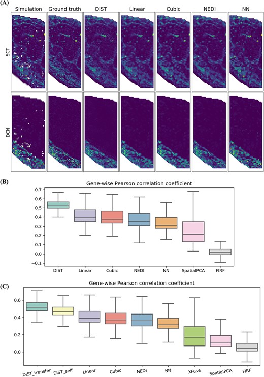
Simulations prove DIST can refine ST profiles with higher accuracy. (A, B) Simulation created from STARmap mouse placenta. (A) Spatial expression of several genes having different spatial patterns based on coarse-resolution simulated data, single-cell-resolution ground truth and imputed data using DIST, Linear, Cubic, NEDI and NN. Consistent color ranges scaled by gene-wise minimum and maximum of ground truth. (B) Gene-wise Pearson correlation correlations between ground truth and imputed expression using DIST, Linear, Cubic, NEDI, NN, SpatialPCA and FIRF. Boxes show 25th, 50th and 75th percentiles. Whiskers indicate the extent of all non-outliers defined as observations within 1.5 interquartile ranges from the hinges. (C) Simulation created from Stereo-seq adult mouse hemi-brain. Gene-wise Pearson correlation correlations between ground truth and imputed expression using DIST_transfer (transfer learning), DIST_self (self-supervised learning), Linear, Cubic, NEDI, NN, XFuse, SpatialPCA and FIRF. Boxes have the consistent explanation with (B).

Open in new tabDownload slide

We calculated PCCs between ground truth and each imputed expression of all spots for the 903 genes and showed the results in Figure 2B. DIST attains higher median of gene-wise PCCs over the best-performing interpolation (median: DIST = 0.523, Linear = 0.389). DIST’s 25th percentile (0.498) of PCCs is even higher than the maximum of 75th percentiles of interpolation methods (Linear = 0.477). We calculated PCCs for SpatialPCA in scaled embedding spaces, since SpatialPCA can only get the imputed scaled data. It is noted that the purpose of SpatialPCA is dimension reduction, not for predicting truth expression values on unmeasured spots. The performance of FIRF is not good, mostly because it is designed for image interpolation and is trained on an image data set.

Next, we created another simulated ST data from Stereo-seq data, which offers subcellular resolution spatial expression on the adult mouse hemi-brain [17]. Similar to the above process, we calculated PCCs between ground truth and imputed expressions from DIST, Linear, Cubic, NEDI, NN, XFuse, SpatialPCA and FIRF (Figure 2C). For DIST, we evaluated imputed values from self-supervised learning and transfer learning trained on IDC data, respectively. In addition, we ran XFuse with a nuclei acid staining image of the tissue section. XFuse can predict pixel-wise expression and get resolution as high as the staining image. To have a comparison, we fused pixels into spots by their locations. Figure 2C reflects that DIST attains the highest median of gene-wise PCCs and transfer learning improves accuracy of prediction. Same as the STARmap simulated data, the PCC of DIST is the highest among all the methods. Because of the shallow sequencing depth, the median of PCCs (0.465) on Stereo-seq simulated data is lower than that on STARmap data for DIST. But after performing transfer learning using a high-quality data, the median of PCCs on Stereo-seq data is improved to 0.518, which is quite close to STARmap data.

Explore spatial patterns of ST human melanoma data

Next, we tested whether DIST can help find spatial patterns for ST. We applied Sepal, a method for identification of transcript profiles that exhibit spatial patterns by diffusion-based model, to an ST data set from human melanoma [7] before and after imputation using DIST. Following the tutorial of Sepal, first, we ranked the gene expression profiles by the degree of spatial structure from distinct to random patterns; then grouped top-ranked genes that had distinct spatial patterns into pattern families, where members of the same pattern family exhibited similar spatial organization; finally subjected the families to functional enrichment analysis querying against the Gene Ontology: Biological Processes (GO: BP) database [36].

Figure 3A shows some top-ranked transcript profiles in the imputed melanoma data but having lower rankings in original melanoma data. CSPG4 is associated with melanoma tumor formation and poor prognosis in certain melanomas [37]. DLL3 is expressed in many metastatic melanomas and targeting the gene may be a promising therapeutic strategy against inflammation-aggravated melanoma progression [38]. CD37 is expressed almost exclusively in cells of the immune system, especially in mature B cells [39]. As shown in Figure 3A, the expressions of these genes have distinct spatial structure. The lower resolution might have led to the relatively low rankings of these genes in original melanoma data. And the DIST imputed HR data allow Sepal to have more power and improve the rankings of these genes significantly.

Figure 3

Explore spatial patterns of ST human melanoma data. (A) Three disease-related genes having higher rankings in imputed data (below) because of distinct spatial patterns but having lower rankings in original data (above). The header of each transcript profile gives the name of the associated gene and ranking. (B) The pathologist’s annotations on hematoxylin- and eosin-stained tissue image from the original paper, where black: melanoma, red: stroma and yellow: lymphoid tissue. (C) The number of genes (left) and significant (P-value < 0.05) GO: BP terms (right) for each family. Green signs numbers from original data; orange signs numbers from imputed data. (D) Top 10 significant GO: BP terms only identified by imputed data in lymphoid (above) and stroma (below) family.

Open in new tabDownload slide

We next asserted top 150 ranked genes into three mainly pattern families and performed enrichment analysis. From representative motifs (Supplementary Figure S2), distinct marker genes (Supplementary Figures S3 and S4) and biological processes for each pattern family, these families can be obviously linked to histological annotations (Figure 3B) including melanoma, lymphoid and stroma. Then we compared these families that had the same spatial patterns on original and imputed ST data. In all, 150 top-ranked genes from imputed ST data were separated into 87 melanoma-related genes, 37 lymphoid-related genes and 25 stroma-related genes, whereas 150 top-ranked genes from original ST data were separated into 108 melanoma-related genes, 31 lymphoid-related genes and 8 stroma-related genes (Figure 3C). For three families, imputed data were enriched more GO: BP terms than original data despite it has less melanoma-related genes (Figure 3C). Moreover, lymphoid family was enriched 124 new pathways, among them multiple processes were related to immune response and lymphocyte activation. Stroma family had more pathways about growth factor (Figure 3D). We also chose 100 or 200 top-ranked genes to repeat the above analytic steps, and they both had consistent results with 150 top-ranked genes (Supplementary Figure S5). It indicates that top-ranked genes from DIST imputed data are more region specific and biologically significant, particularly in lymphoid. Lymphoid region and stroma region are relatively smaller than melanoma region. Because of the LR and small region, lymphoid-related genes and stroma-related genes have much lower rankings compared with larger region such as melanoma. DIST improves the resolution and thereby Sepal has more power to find those lymphoid- and stroma-related genes.

Explore biological functions of Visium human IDC data

We further analyzed the human IDC sample prepared on the Visium platform following the subsequent analyses including clustering, differential expression analysis and pathway enrichment. We were interested in what new discoveries DIST could bring compared with original ST data.

We tried two strategies to train our model. First, we used the basic self-supervised learning scheme, training set and test set were from the same ST data. The result shows that new imputed spots cannot merge well with original spots on clusters, leading to phenomenon like batch effect (Figure 4A). This might be because DIST cannot be well trained because of the low quality of IDC data. So, we next tried the transfer learning scheme, training on a better-quality data. Here, we used Visium mouse sagittal posterior brain data [40] to construct training set. The mean reads number per spot of mouse sagittal posterior brain data is 87 128 [40], whereas that of IDC is only 40 795 [29]. The clustering result of imputation is visually smooth and consistent with that of original data (Figure 4B). It indicates that DIST can improve the imputed result of low-quality data by leveraging information learnt from high-quality data. The high-quality data have less noises, hence transfer learning allows DIST to avoid excessive noises to improve the accuracy of imputation. The following analyses are based on results from transfer learning.

Figure 4

Compare clustering results of Visium human IDC data. (A, B) Louvain clustering displays of imputed Visium human IDC using two strategies. (A) Based on self-supervised learning strategy. (B) Based on transfer learning model trained on a high-quality data, Visium mouse sagittal posterior brain. (C) Clustering performance of original (orange) and imputed (blue) IDC in obtaining smooth and continuous spatial domains measured by LISI. Lower LISI score indicates more homogeneous and continuous spatial structure. (D) Domains from original expression. (E) Merged version of (B), having matched domains with (D) by the same color.

Open in new tabDownload slide

First, we compared clustering results of IDC before and after DIST imputation (Figure 4B and D and Supplementary Figure S6). The results show that the DIST imputed expression has smoother clustering result. We clustered original and imputed expression using different numbers of PCs and resolutions by Louvain algorithm. The spatial domains detected on imputed IDC are intuitively more continuous and smoother (Figure 4B and Supplementary Figure S6), which is also confirmed by lower local inverse Simpson’s indexes (LISIs) [41] (Figure 4C). The median of LISIs based on original expression is greater than that based on imputed expression for every parameter combination. The minimum median of LISIs based on original expression is 1.709, even greater than the maximum median of LISIs based on imputed expression that is 1.510. Figure 4B and D shows the clustering results using 15 PCs and 0.8 resolution, which was used for further differential expression analysis and functional enrichment analysis.

Differential expression analysis results show there are more meaningful markers found from imputed expression than original data. For ease of comparison between the original and imputed IDC, we manually merged domains to form one-to-one mapping between the two clustering results (Figure 4D and E). In almost all spatial domains, imputed IDC can find more significant DE genes than original data (Figure 5A). The numbers of overlapped DE genes are close to those of original transcriptomic data for every domain, which suggests that DIST can help identify more significant DE genes while preserving the information of the original data. In addition, we analyzed a matched single-cell RNA-seq data of IDC [42] as reference and verified that larger numbers of significant DE genes were not caused by false positives (Figure 5B). We considered DE results of single-cell RNA-seq more credible since it has deep sequencing depth and single-cell resolution. Here, we used Seurat label transfer method to map each cell into spatial domains [43]. In six comparisons between carcinomas and immune domains, imputed IDC has more significant DE genes, and its overlaps with single-cell reference are also much more than original data, indicating that DIST can find more true DE genes.

Figure 5

Explore biological functions of IDC data. (A) The number of significant (adjusted P-value < 0.05 and log2-foldchange > 1) DE genes for each domain. Green signs numbers from original data; orange signs numbers from imputed data; gray signs the overlaps of both. (B) The number of significant DE genes for compared pairs and overlaps with single-cell reference. (C) The pathologist’s annotations on immunofluorescent tissue image from [18], where red: invasive carcinoma, yellow: carcinoma in situ, green: benign hyperplasia and gray: unclassified tumor. (D) Top 10 significant GO: BP terms only identified by imputed data in domain 0 (above) and domain 10 (below).

Open in new tabDownload slide

According to immunofluorescent imaging and histopathological annotations of the tissue section [18] (Figure 5C), the 12 domains can be categorized into invasive carcinoma (label: 0,4,7,8), carcinoma in situ (label: 3,9), benign hyperplasia (label: 2) and immune response-related domains (label: 1,5,6,10,11). In disease-related domains, several carcinomas-related genes were found in DE genes from imputed data, but not original data. For example, EZH2 [44] and SOCS1 [45] in domain 0 and AKT1 [46] in domain 4 are well known markers of IDC [47]. In immune-related domain 10, newly identified DE genes include ADA, an enzyme that can enhance CD4+ T-cell differentiation and proliferation: IGHG1 and IGHG4, predicted to be involved in the activation of immune response and phagocytosis [47].

To further explore biological functions, these domains were subjected to functional enrichment analysis querying against the GO: BP database. Imputed expression brought some new discoveries. For example, there were pathways associated with chromosome organization and DNA metabolic process enriched in domain 0, which were related to cell growth in carcinoma (Figure 5D). In domain 10, multiple processes including B cell, T cell, leukocyte activation and positive regulation involved in immune response were enriched significantly (Figure 5D).

Figure 6

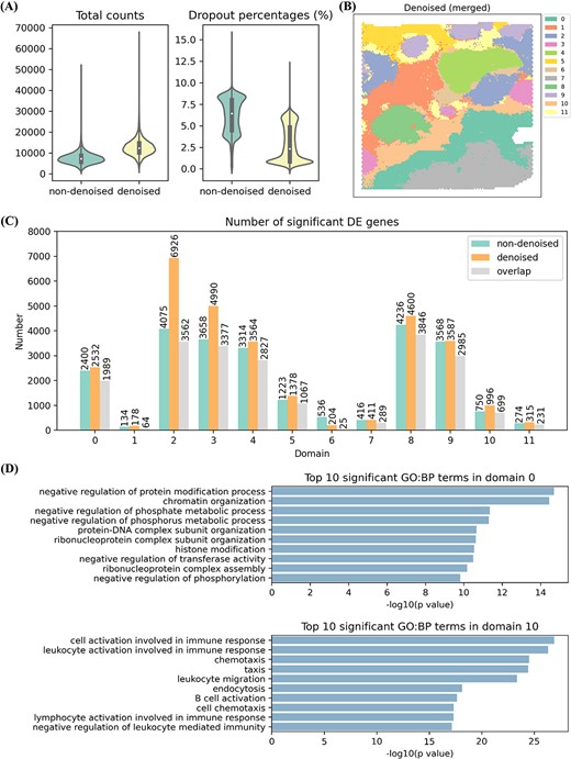
DIST simultaneously imputes and denoises low-quality IDC. (A) The violin plot of total counts (total number of counts for each spot) (left) and dropout percentages (percentage of spots each gene does not appear in) (right) based on non-denoised imputed IDC (light green) and denoised imputation (light yellow). (B) Merged clustering result of denoised imputation (Supplementary Figure S7), having matched domains with Figure 4E by the same color except for domains 1 and 6. (C) The number of significant (P-value < 1×10^-6 and log2-foldchange > 0.6) DE genes for each domain. Green signs numbers from non-denoised data; orange signs numbers from denoised data; gray signs the overlaps of both. (D) Top 10 significant GO: BP terms only identified by denoised data in domain 0 (above) and domain 10 (below).

Open in new tabDownload slide

DIST denoises Visium human IDC data

Transfer learning can improve the accuracy of imputation, but cannot reduce noises of imputed expression. In this section, we show how to use DIST to denoise the imputed expression by adding an additional step.

Because of low amounts of RNA sequenced within individual spots, low-quality ST data are usually noisy and sparse, leading to masked biological signals. For these noisy and sparse data, DIST can not only improve the imputation by transfer learning, but also denoise the imputed expression to increase the depth of UMI counts and decrease the rate of dropouts. Denoising could be implemented by an additional step, introducing synthetic noises to the inputs during the training process. The LR inputs have more noises than their HR ground truth, so DIST can learn how to simultaneously impute and denoise low-quality data.

We indicated the effect of noise reduction based on discussed IDC by comparing with non-denoised imputation of the previous section. We compared the total number of UMI counts for each spot and percentage of spots with zero UMI count for each gene between denoised expression and non-denoised expression. The results are shown in Figure 6A. The mean of total counts of denoised expression improves from 7237 to 12 367 and the mean of dropout percentages of denoised expression reduces from 6 to 2%. The quality of denoised expression improves significantly in terms of total UMI counts and percentages of dropouts.

Next, we analyzed denoised data by the same procedure as non-denoised data including clustering, differential expression analysis and pathway enrichment. Denoised data have similar clustering result to non-denoised data (Figures 4E and6B). We found more DE genes from denoised data than non-denoised data for every matched domain (Figure 6C). In disease-related domains, several well-known markers are included in DE genes from denoised data, but not non-denoised data. Examples of such genes are: NCOA4 [48] and SOCS1 [45] in domain 0, ADGRB1 [49] in domain 4, well-known markers of IDC [47]; HOXB13 [50] and KLK10 [51] in domain 3, two markers of ductal carcinoma in situ [47]. Moreover, we found some GO terms enriched in the upregulated DE genes that could be only detected in the denoised data, but not in the non-denoised data. These enriched terms are highly relevant to the biological functions of carcinoma and immune reaction. For example, there were pathways associated with protein and phosphate enriched in domain 0 (Figure 6D). And multiple processes related to immune response were enriched significantly in domain 10 (Figure 6D). In total, the denoising can reduce the noise of imputed expression and strength the power of identifying significant DE genes and biological signals.

In addition, we used different efficiency loss |$\lambda$| to investigate how the different synthetic noise levels impacted denoising performance. Efficiency losses |$\lambda$| = 0.2, 0.4, 0.6 and 0.8 were selected and the results are shown in Supplementary Figure S8. With the decreasing of efficiency loss, more noises were introduced to the inputs, and the denoised imputation had deeper sequencing depth. From the clustering results, smaller efficiency loss leads to smoother domains and the lack of details. Hence, it is appropriate to take efficiency loss larger than 0.5 to avoid the lack of original details.

Discussion

We developed DIST, a deep learning-based method that enhances ST data by self-supervised learning and transfer learning. Through self-supervised learning, DIST can impute the gene expression levels at unmeasured area accurately and improve the data quality in terms of total counts and dropout percentages. Moreover, transfer learning enables DIST improve the imputed gene expression by borrowing information from other high-quality data. It is worth noting that the informative high-quality data do not have to come from the same tissues or species as target ST data, as we enhanced poor quality human IDC data by the model trained on good quality mouse brain data. We also used different species or tissues data as sources to perform the transfer learning on IDC data, the results show (Supplementary Figure S9) that the sources from the same species lead to better performance, but the difference is minor. Even from different species or tissues, DIST still can learn enough knowledge from the source to improve the prediction performance.

In spatially resolved transcriptomics studies, identifying genes that display spatial expression patterns is an essential step toward characterizing the ST landscape in complex tissues [21]. Gene expression profiles that possess distinct spatial patterns are of particular interest when attempting to chart the biological processes and pathways present within a tissue using transcriptome-wide techniques [52]. Because of the low statistical power, it is hard to find the biological meaningful genes with spatial patterns in small size region with LR transcriptomics data. Through analyzing ST human melanoma data, we illustrated that DIST allowed us to detect more genes with distinct spatial patterns in small regions and make small region-specific genes, such as lymphoid- and stroma-related genes having much higher rankings compared with original data. Besides LR, noise such as shallow sequencing depth or dropout events is another reason for loss of power to explore biological significance. In Visium IDC data analysis, we showed that DIST could improve the total UMI counts and reduce the dropouts by denoising and using DIST enhanced data we could find more DE genes and thereby find more significant enriched pathways.

To quantify the cost of time and memory of DIST, we recorded the time and memory usage of NN, DIST, Linear, Cubic, NEDI, SpatialPCA and XFuse on the same ST data. The results are shown in Supplementary Table S1. DIST is the second fastest method and only takes <2 min to finish the whole process.

While our evaluations were performed on ST and Visium platforms, DIST should be applicable to other platforms such as Stereo-seq [17]. We applied DIST to Stereo-seq data from mouse embryo at E9.5 and the results are shown in Supplementary Figure S10. Same as IDC data, DIST improved the total counts significantly and found more significant DE genes than original data. Besides, while our work focused on two-dimensional tissue slices and their gene expression, DIST could be extended to three-dimensional (3D) ST reconstruction that provides more comprehensive perspective to biological exploration. For reconstructing 3D expression, existing methods usually align and integrate ST data from multiple adjacent tissue slices [53]. Some imputed approaches cannot be easily applied to 3D expression, since there is no matched histology image between tissue slices. However, DIST only need gene expression and spot coordinates therefore it could be applicable to 3D expression with slight modifications to network parameters and the dimension of VLN inputs. In summary, DIST offers comprehensive data enhancement including imputation and denoising and could be a useful tool for ST data analysis.

Data availability

Data sets analyzed in this paper are available from their original publications. The STARmap mouse placenta is available at Code Ocean https://codeocean.com/capsule/9820099/tree/v1 [33]. The human melanoma ST data (mel1 rep1) can be found at https://www.spatialresearch.org/resources-published-datasets/doi-10-1158-0008-5472-can-18-0747 [7]. Raw count matrix, histology image and spatial data from the IDC sample are accessible on the 10x Genomics website at https://www.10xgenomics.com/resources/datasets/invasive-ductal-carcinoma-stained-with-fluorescent-cd-3-antibody-1-standard-1-2-0 [29]. Relevant information about the mouse sagittal posterior brain sample is accessible at https://www.10xgenomics.com/resources/datasets/mouse-brain-serial-section-1-sagittal-posterior-1-standard-1-1-0 [40]. Stereo-seq data from the adult mouse hemi-brain and mouse embryo are both from MOSAT database at https://db.cngb.org/stomics/mosta/.

Code availability

An open-source implementation of the DIST algorithm can be downloaded from https://github.com/zhaoyp1997/DIST.

Funding

This work was supported by National Natural Science Foundation of China (31970649) to G.H. and K.W.

Yanping Zhao is a graduate student at School of Statistics and Data Science, Nankai University. Her research interests include statistical genomics and muti-omics analysis.

Kui Wang is an associate professor at School of Statistics and Data Science, Key Laboratory for Medical Data Analysis and Statistical Research of Tianjin, Nankai University. His research interests include structural bioinformatics, single-cell RNA sequencing analysis, and the application of deep learning in bioinformatics.

Gang Hu is a professor at School of Statistics and Data Science, Key Laboratory for Medical Data Analysis and Statistical Research of Tianjin, Nankai University. His research interests include structural bioinformatics, statistical genomics, and multi-omics analysis.

References