


Abstract
Identifying proteins that interact with drugs plays an important role in the initial period of developing drugs, which helps to reduce the development cost and time. Recent methods for predicting drug–protein interactions mainly focus on exploiting various data about drugs and proteins. These methods failed to completely learn and integrate the attribute information of a pair of drug and protein nodes and their attribute distribution.
We present a new prediction method, GVDTI, to encode multiple pairwise representations, including attention-enhanced topological representation, attribute representation and attribute distribution. First, a framework based on graph convolutional autoencoder is constructed to learn attention-enhanced topological embedding that integrates the topology structure of a drug–protein network for each drug and protein nodes. The topological embeddings of each drug and each protein are then combined and fused by multi-layer convolution neural networks to obtain the pairwise topological representation, which reveals the hidden topological relationships between drug and protein nodes. The proposed attribute-wise attention mechanism learns and adjusts the importance of individual attribute in each topological embedding of drug and protein nodes. Secondly, a tri-layer heterogeneous network composed of drug, protein and disease nodes is created to associate the similarities, interactions and associations across the heterogeneous nodes. The attribute distribution of the drug–protein node pair is encoded by a variational autoencoder. The pairwise attribute representation is learned via a multi-layer convolutional neural network to deeply integrate the attributes of drug and protein nodes. Finally, the three pairwise representations are fused by convolutional and fully connected neural networks for drug–protein interaction prediction. The experimental results show that GVDTI outperformed other seven state-of-the-art methods in comparison. The improved recall rates indicate that GVDTI retrieved more actual drug–protein interactions in the top ranked candidates than conventional methods. Case studies on five drugs further confirm GVDTI’s ability in discovering the potential candidate drug-related proteins.
[email protected]Supplementary information: Supplementary data are available at Briefings in Bioinformatics online.
1 Introduction
Drugs usually perform their functions by forming interactions with all sorts of molecular targets, among which proteins are a major class of targets [1, 2]. In the incipient stage of drug development, the identification of drug–target interactions (DTIs) is particularly important [3–6]. However, the identification of DTIs is a time-consuming and costly process [7]. Therefore, various calculation methods have been exploited to infer possible DTIs, providing biologists with information regarding drug-related protein candidates and reducing the workload of wet experiments [8–11].
Early calculation methods for determining drug–protein interactions are mainly divided into two categories. The first category comprises molecular-docking-based methods [12–14], which use the three-dimensional structure of the protein to predict DTIs. However, the three-dimensional structure of many proteins, such as the membrane protein GPCR [15, 16], is not available; this limits the performance of such approaches. The other category comprises ligand-based methods [17], which compare proteins with unknown ligands and those with known ligands. However, when the number of known binding ligands is small, these methods do not work well.
Over the years, computational methods based on machine learning have been proposed to predict drug–protein interactions. Ding et al. established a drug–protein interaction prediction model based on support vector machines, which mainly used the substructure fingerprint of drugs, the physical and chemical properties of the target organism, and the relationships between drugs and target proteins [18]. A support vector machine (SVM) framework based on bipartite local models (BLMs) was proposed by Bleakley and Yamanishi to predict drug–protein interactions [19]. DDR is established based on the random forest algorithm, which mainly utilizes the similarity information and interaction information of drugs and proteins for DTI prediction [20]. Xuan et al. proposed an approach, DTIGBDT, establishing a drug–protein interaction prediction model based on a gradient boosting decision tree (GBDT) [21].
However, most of these methods only use the similarity information and interaction information of drugs and proteins, and do not use other data sources. An information flow-based method is proposed to predict drug-related proteins [22]. DTINet, which mainly utilizes multifarious relationships among drugs, proteins and diseases to study the low-dimensional vector representation of nodes for predicting DTIs, has also been constructed [23]. There are complex correlations between various data regarding drugs and proteins. However, because most of the aforementioned approaches are shallow predictive models, it is difficult to learn such correlations using these methods.
Several recent prediction methods focus on building models based on deep learning to enhance the accuracy of the prediction of drug-related proteins. Sun et al. established a drug–protein interaction prediction model based on generative adversarial networks [24]. An ensemble learning method based on non-negative matrix factorization and GBDT was proposed to infer candidate proteins interacting with drugs [25]. Based on the Weisfeiler-Lehman Neural network, a drug–protein interaction prediction model is established; this model deeply fuses the similarity and interaction information of drugs and proteins [26]. The relationships of the associations among drugs, proteins and diseases also represent essential ancillary information for predicting drug–protein interactions. However, these methods fail to take advantage of information regarding drug-related and protein-related diseases. Zhang et al. established a model for drug–protein interaction prediction based on bidirectional gated recurrent unit, which deeply integrated multiple data related to drugs, proteins and diseases. However, this method failed to take into account the attribute distribution of node pairs [27].
To tackle the limitations in existing conventional methods for drug–protein interaction prediction, we propose a new model, GVDTI, to learn and integrate three pairwise representations from multi-source data, including the attention-enhanced topological representations, attribute distributions and attribute representations. The contributions of our model include:
To extract attention-enhanced topological structure and node attributes, we propose a graph convolutional autoencoder (GCA) based framework and an attribute-level attention mechanism. GCA extracts and embeds the hidden topological structure from drug similarity, drug–disease and drug–protein sub-networks. Since individual attribute in a node’s attribute vector have different contributions to topological embedding, we propose the new attention mechanism at node attribute level to adaptively learn and reflect the discriminative contributions of each sub-network’s node attribute.
To facilitate the extraction of attribute distribution and attribute representation of drug–protein node pairs, we first construct a drug–protein–disease heterogeneous network and an embedding strategy to associate the similarities, interactions and associations of pairs of nodes. The embedding strategy reflects the biological premise that a pair of drug and protein nodes is more likely to interact with each other if they share more common drugs, proteins or diseases.
We propose a novel convolutional variational autoencoder (CVAE) based approach to learn pairwise attribute distributions. The attribute distribution reveals the underlying drug–protein relationship in the established drug–protein–disease heterogeneous network by a convolutional variational encoding and decoding process to foster the prediction of drug-related proteins.
To extract drug–protein pairwise attribute representation, we design a new encoding strategy based on the multi-layer convolutional neural network (MCNN). The pairwise attribute representation integrates the similarities, interactions and correlations of a pair of drug and protein nodes. The ability of the proposed model, the learnt attention-enhanced topological representations, attribute representations and attribute distributions for drug–protein interaction prediction are demonstrated by comprehensive comparison with recently published models and case studies of five drugs.
2 Materials and Methods
Figure 1 demonstrates the framework of our model for predicting drug–protein interactions. First, we constructed a module based on graph convolutional networks with attention to capture the topology structures of multiple subnets, and the module learned the topology representation of each drug node and that of each protein node. Second, a tri-layer heterogeneous network composed of drug nodes, protein nodes and disease nodes was constructed. The attribute distribution representation and the attribute representation of a drug–protein node pair were encoded separately. Finally, these three representations were deeply fused to get the interaction score of the node pair.
2.1 Dataset
In this paper, the protein–disease associations, the drug–disease associations, the drug–protein interactions, the drug similarities and the protein similarities were obtained from a previously published paper [23]; the information obtained included 708 drugs, 1512 proteins, 5603 diseases, 199 214 known drug–disease associations, 1596 745 known protein–disease associations and 1923 known drug–protein interactions. The associations among proteins, drugs and diseases were originally obtained from the comparative toxigenics database (CTD), which mainly provides information about the relationships among chemistry, genes and diseases [28].
2.2 Calculation and representation of multi-source data
Five types of matrices are defined to represent data regarding drugs, proteins and diseases, including similarity matrices of drugs and proteins, drug–disease association matrix, protein–disease association matrix and drug–protein interaction matrix.
2.2.1 Association and interaction matrices
As shown in Figure 2, we use matrix |$A^{drug} \in{\mathbb{R}^{n_{r} \times{n_{d}}}}$| to represent the associations between |$n_{r}$| drugs and |$n_{d}$| diseases, where if drug |${r_{i}}$| is observed to be associated with disease |${d_{j}}$|, then |$A_{ij}^{drug}$| is 1 (otherwise, it is 0). The protein–disease association matrix is denoted by |$A^{protein} \in{\mathbb{R}^{n_{p} \times{n_{d}}}}$|, and the matrix element |$A_{ij}^{protein}$| is 0 or 1. 1 indicates that the protein is related to disease, while 0 indicates the opposite. The matrix |$Y \in{\mathbb{R}^{n_{r} \times{n_{p}}}}$| represents the interactions between drugs and proteins. When |$Y_{ij}$| is 1, it means that the interaction between drug |${r_{i}}$| and protein |${p_{j}}$| is observed, otherwise, it is 0.
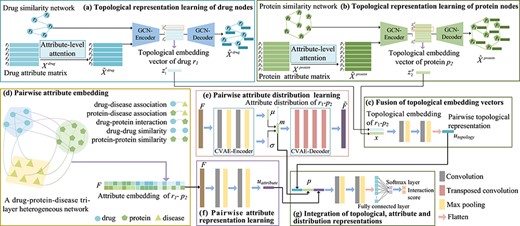
The framework of the proposed GVDTI model, take |${r_{1}}$| and |${p_{2}}$| as examples. The topological embedding vector of each drug or protein node is learned by a graph convolutional autoencoder (a) and (b), and the multi-layer convolutional neural network is used to fuse the topology embedding of |${r_{1}}$| - |${p_{2}}$|(c). (d) A tri-layer heterogeneous network is constructed, and the proposed embedding strategy is used to form an attribute-embedding matrix of |${r_{1}}$| - |${p_{2}}$|. (e) Pairwise attribute distribution representation is extracted using a convolutional variational autoencoder. (f) Pairwise attribute representation is obtained by multi-layer convolutional coding. (g) Fusion of the three pairwise representations, attention-enhanced topological representation, attribute distribution and attribute representation.
2.2.2 Similarity matrices
Based on the chemical substructure information of drugs, the authors of a previous study calculated the intra drug similarity using Tanimoto coefficient [29]. In Figure 2, matrix |$S^{drug} \in{\mathbb{R}^{n_{r} \times{n_{r}}}}$| is used to represent the similarity matrix of drugs, and |$S_{ij}^{drug} \in [0,1]$| is the similarity value between drug |${r_{i}}$| and drug |${r_{j}}$|. The larger the |$S_{ij}^{drug}$|, the higher the similarity between drug |${r_{i}}$| and drug |${r_{j}}$|. As shown in Figure 2, the protein similarity matrix |$S^{protein} \in{\mathbb{R}^{n_{p} \times{n_{p}}}}$|, which was described in [30], was constructed on the basis of the Smith–Waterman score based on the primary sequences of the targets. |$S_{ij}^{protein}$| indicates the similarity value between protein |${p_{i}}$| and protein |${p_{j}}$|.
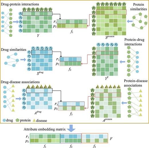
Similarity matrices, interaction matrices and association matrices derived from corresponding networks of drugs, proteins and diseases. The detailed process of the proposed embedding strategy. Considering drug |${r_{1}}$| and protein |${p_{2}}$| as examples, the attribute-embedding matrix of |${r_{1}}$| - |${p_{2}}$| is constructed.
2.3 Pairwise attention-enhanced topological representation learning
2.3.1 Attention mechanism at attribute level

Extraction and fusion of the topological embedding of |${r_{1}}$| - |${p_{2}}$|.
2.3.2 Pairwise attention-enhanced topology extraction by graph convolutional autoencoder
Homoplastically, we also need to fuse the protein attribute matrix |$\widetilde{X}^{protein}$| and similarity matrix |$S^{protein}$| and extract the low-dimensional topological representation of the protein to obtain matrix |$Z^{p}$|.
Let |$z_{1}^{r}$| be the first row of |$Z^{r}$| and |$z_{2}^{p}$| be the second row of |$Z^{p}$|. Taking drugs |$r_{1}$| and protein |$p_{2}$| as examples, we stacked the topological embedding vector |$z_{1}^{r}$| of the drug node and the topological embedding vector |$z_{2}^{p}$| of the protein node up and down to obtain
2.4 Construction of attribute-embedding matrix
The biological premise of our embedding strategy is that if a pair of drug and protein nodes have interactions, associations or similarities with more of the same drugs, proteins or diseases, the said pairs of nodes are more likely to interact. Based on this biological premise, we established pairwise attribute-embedding matrices, for example, the attribute-embedding matrix of |${r_{1}}$|-|${p_{2}}$|.
2.5 Pairwise attribute distribution learning by CVAE
A CVAE is a deep generative model [35]. Unlike traditional autoencoders [36], which describe the low-dimensional feature representation of |${r_{1}}$|-|${p_{2}}$| numerically, a CVAE describes this in a probabilistic way, and finally yields the pairwise attribute distribution representation |$m$|.
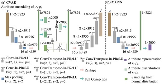
shows the process for the extraction of the pairwise attribute distribution and attribute representation of |${r_{1}}$|-|${p_{2}}$|.
2.6 Pairwise attribute representation learning by multi-layer convolutional neural network
2.7 Integration of the multiple pairwise representations
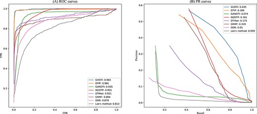
ROC curves and PR curves of all the methods in comparison of all the 708 drugs.
3 Experimental evaluations and discussions
3.1 Evaluation metrics
In this article, we treated the known drug–protein interaction samples as positive samples, and the unknown drug–protein interactions as the negative samples. In our dataset, there are 1923 positive samples and |$708 * 1512 - 1923 = 1068\,573$| negative samples. Obviously, there is a serious class imbalance between the positive and negative samples. Therefore, we randomly extracted negative samples at the same amount as the positive samples and formed the set A together with the positive samples. Set B contains |$1068\,573-1923=1066\,650$| negative samples.
We utilized 5-fold cross-validation to evaluate the performance of GVDTI and several other more advanced forecasting methods. The same training data and test data were used to verify these methods. In every cross-validation, we randomly divided the samples in set A into five equal subsets, four of which are for training; the fifth subset is combined with set B as the test set.
The statistical results of the paired Wilcoxon test on the AUCs and AUPRs over all the 708 drugs by comparing GVDTI and all other seven methods.
| DTIP | GANDTI | NGDTP | DTINet | GRMF | DDR | Lee’s method | |
|---|---|---|---|---|---|---|---|
| p-value of AUC | 1.2215e-153 | 0.2123e-112 | 2.2055e-133 | 5.0918e-62 | 3.5449e-75 | 2.5239e-92 | 5.1732e-89 |
| p-value of AUPR | 5.1432e-294 | 7.6154e-134 | 6.6362e-261 | 8.5746e-224 | 2.9768e-249 | 1.5273e-104 | 1.0503e-114 |
The top 10 candidate proteins of five drugs
| Drug name | Rank | Targets | Evidence | Rank | Targets | Evidence |
|---|---|---|---|---|---|---|
| 1 | HTR6 | DrugBank/STITCH | 6 | DRD5 | DrugBank | |
| 2 | CHRM2 | DrugBank | 7 | ADRA2C | DrugBank | |
| Quetiapine | 3 | CHRM4 | DrugBank | 8 | ADRA1B | DrugBank |
| 4 | HTR2C | DrugBank/STITCH | 9 | CHRM5 | DrugBank | |
| 5 | ADRA1D | DrugBank | 10 | DRD2 | DrugBank/STITCH | |
| 1 | HTR2C | DrugBank/STITCH | 6 | NR1I2 | Unconfirmed | |
| 2 | HTR7 | DrugBank/STITCH | 7 | CHRM1 | DrugBank/STITCH | |
| Clozapine | 3 | HTR1D | DrugBank | 8 | ADRA1A | DrugBank |
| 4 | HTR6 | DrugBank/STITCH | 9 | CHRM5 | DrugBank | |
| 5 | HTR1B | DrugBank | 10 | HRH4 | DrugBank | |
| 1 | KCNJ11 | DrugBank | 6 | CACNA1A | DrugBank | |
| 2 | ADRA2B | Unconfirmed | 7 | CACNA1B | DrugBank | |
| Verapamil | 3 | KCNH2 | DrugBank/STITCH | 8 | CACNB4 | Literature [49] |
| 4 | CACNB2 | Literature [49] | 9 | CACNA1C | DrugBank/STITCH | |
| 5 | CACNA1S | Literature [49] | 10 | CACNA1F | Literature [49] | |
| 1 | CHRM2 | DrugBank | 6 | SLC6A2 | DrugBank | |
| 2 | NTRK1 | DrugBank | 7 | HTR2A | DrugBank/STITCH | |
| Amitriptyline | 3 | KCNQ2 | DrugBank | 8 | KCND2 | Literature [50] |
| 4 | KCNA1 | DrugBank | 9 | OPRD1 | DrugBank | |
| 5 | ADRA1A | DrugBank/STITCH | 10 | KCND3 | Literature [50] | |
| 1 | HTR2C | DrugBank/STITCH | 6 | HTR3A | DrugBank | |
| 2 | DRD2 | DrugBank | 7 | CHRM3 | DrugBank | |
| Ziprasidone | 3 | DRD5 | DrugBank | 8 | ADRA2C | Literature [51] |
| 4 | ADRA2A | DrugBank | 9 | HRH2 | Unconfirmed | |
| 5 | HTR1D | DrugBank/STITCH | 10 | HTR6 | DrugBank |
3.2 Comparison with other methods
The performance of the proposed GVDTI method for drug–protein interaction prediction is compared with that of several advanced methods, including DTIP [27], GANDTI [24], NGDTP [25], DTINet [23], GRMF [46], DDR [20] and Lee’s method [47]. As shown in Figure 5(A), GVDTI achieved the highest average AUC (AUC = 0.983) of all the 708 tested drugs, which is 0.2% higher than that of the model showing second-best performance, DTIP, 2.8% higher than that of NGDTP, 4.8% higher than that of GANDTI, 6.2% higher than that of DTINET, 8.9% higher than that of GRMF, 10.4% higher than that of DDR and 17.1% higher than that of the worst-performing method, i.e. Lee’s method. The GVDTI method showed the best performance, achieving an AUPR of 0.435, which is superior to that of DTIP, NGDTP, GRMF, DTINet, GANDTI, Lee’s method and DDR by 3.6%, 7.4%, 11.6%, 26%, 36.1%, 37.6% and 38.5%, respectively.
DTIP showed the second-best performance. Based on bidirectional GRU, this method learns the multi-scale neighbor topology of drugs and proteins, and deeply explores the potential relationship between drugs and proteins. NGDTP also showed a good performance. Based on non-negative matrix factorization, this method fuses multiple connection data between drugs and proteins, learning the topological representation of drugs and proteins. These findings indicate that it is necessary to integrate various information about drugs and proteins to obtain the topological representation of nodes.
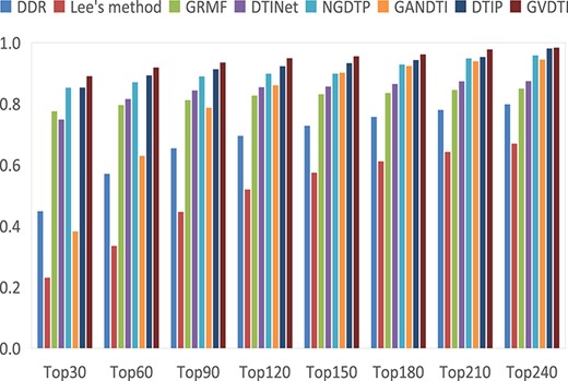
The average recalls over all the drugs at different top |$k$| values.
DTINet performed well with regard to the AUC (AUC = 0.921), but it did not achieve a good AUPR (AUPR = 0.175). On the contrary, GRMF achieved a good AUPR (AUPR = 0.319), but its AUC was a little worse (AUC = 0.894). NGDTP, DTINet and GRMF are all shallow prediction models based on matrix factorization; these cannot deeply learn the complex associations between the information regarding various drugs and proteins. Based on the generative adversarial network, GANDTI established a drug–protein interaction prediction model. However, this approach does not utilize drug–disease associations and protein–disease associations. DDR and Lee’s method performance was even worse, because the former does not use network topology information and the latter ignores the attribute information of the node. Our method not only performed the in-depth fusion of a variety of information related to the drugs and proteins, but also made the most of the attribute messages of the nodes.
In addition, for each prediction method, we obtain 708 AUCs and 708 AUPRs for all the 708 drugs. We performed Paired Wilcoxon test on the 708 paired AUCs or AUPRs of every two methods. Wilcoxon tests were used to assess whether the AUCs and AUPRs of GVDTI were significantly greater than each of the other seven approaches for the 708 drugs. Table 1 shows that GVDTI with regard to the AUCs and the AUPRs was significantly better than the other methods (|$p$|-value < 0.05).
Among the top k protein candidates of the prediction results, the higher the recall rate, the more correctly will real proteins be identified. Under different k values, GVDTI’s performance was always better than that of the other methods (Figure 6), accounting for 89.7% of the positive samples in the top 30, 91.8% in the top 60 and 94.9% in the top 120. The recall rates of DTIP ranked second, with 85.3%, 89.4% and 93.5% positive samples in the top 30, 60 and 120, respectively. GANDTI identified 38.2%, 62.9% and 86.1% of the positive samples in the top 30, 60 and 120, respectively. NGDTP identified 85.2%, 87.1% and 89.8% of the positive samples in the top 30, 60 and 120, respectively. DTINet identified 74.8%, 81.5% and 85.4% of the positive samples in the top 30, 60 and 120, respectively, which were slightly higher than those of the GRMF method (77.5%, 79.5% and 82.6%, respectively). In contrast, Lee’s method was inferior to other methods, identifying 23%, 33.4% and 51.9%, respectively.
3.3 Case studies on five drugs
To fully prove the ability of GVDTI to discover potential drug–protein interactions, we conducted case studies on five drugs (quetiapine, verapamil, amitriptyline, clozapine and ziprasidone), and each of drug has at least 14 known drug–protein interactions. We collected and analyzed the top 10 candidate proteins for each drug (Table 2). In addition, we also conducted case studies on five drugs (imipramine, triazolam, desipramine, clonazepam, diazepam) each of which has less than 14 known drug–protein interactions. We collected their top five candidates and listed them in supplementary Table ST1.
The DrugBank database not only contains detailed drug data, such as chemical data and pharmacological data, but also includes comprehensive drug–protein data, such as information regarding their sequence, structure and pathway of action [46]. STITCH (Search Tool for Interacting Chemicals), which is a database based on Compartments: cellular localizations, eggNOG: gene orthology and STRING: protein–protein networks, contains detailed protein-related data, drug-related data and information regarding drug–protein interactions. As shown in Table 2, 40 candidate proteins were recorded by DrugBank and 13 candidate proteins were identified by STITCH. This result shows that these candidate proteins do interact with the corresponding drugs.
Four candidate proteins of verapamil, two candidate proteins of amitriptyline and one candidate protein of ziprasidone are labeled as ‘literature’. They have been confirmed by several published articles; this validates their mutual interaction. Of the 50 candidate proteins, three were marked as ‘unconfirmed’.
The top five candidates for five drugs each of which has less than 14 known drug–protein interactions were listed in supplementary Table ST1. The Kyoto Encyclopedia of Genes and Genomes (KEGG) is a database which contains the detailed drug data, the protein data and the drug–protein interactions. The Comparative Toxicogenomics Database (CTD) is also a public database that includes the drug–protein interactions. Five candidate proteins were recorded by KEGG, and four candidate proteins were included by CTD. The databases, DrugBank and STITCH, covered 16 and 10 candidates, respectively. It indicates that these candidates indeed interact with their corresponding drugs. In these 25 candidates, only two candidates were marked as ‘unconfirmed’, which means there are no evidences to confirm their interactions. The above analysis indicates that GVDTI has the powerful ability in discovering potential drug–protein interactions.
3.4 Prediction of novel proteins related to drugs
After training the prediction model using all drug–protein interrelationships, we used it to predict the top 10 ranked protein candidates for each drug and provide it in the supplemental Table ST2 (https://github.com/pingxuan-hlju/GVDTI). This may help biologists identify actual drug-related proteins through wet laboratory experiments.
4 Conclusions
We propose a novel prediction method, GVDTI, which extracts and integrates the topological structure of multiple sub-networks of drugs and proteins, as well as the attribute distribution and attribute representation of drug–protein node pairs to predict drug-related candidate proteins. GVDTI captures the various intra-relationships between drugs and proteins, i.e. drug similarities and protein similarities. Simultaneously, it captures the inter-relationships among drugs, proteins and diseases, i.e. drug–protein interactions, drug–disease associations and protein–disease associations. The developed graph convolutional autoencoder based framework learns pairwise topological representation, attribute distribution and attribute representation. The node attribute attention mechanism distinguishes the contributions of different attributes of a drug or protein node from its topological embedding vector. The tri-layer heterogeneous network is conducive to the formulation of pairwise attribute-embedding and further promotes the learning of pairwise attribute distribution and attribute representation. The experimental results demonstrated that GVDTI improved the drug–protein candidates prediction and top candidate proteins identification results. Our model can be used as a tool to screen potential candidate proteins and then discover the real drug–protein interaction relationships through wet laboratory experiments.
A newly proposed attention-enhanced pairwise topological representation to embed the topology structure of drug and protein nodes and reveal the underlying topological relationship of drug–protein sub-networks. The attribute-level attention mechanism distinguishes the different contributions of various attributes of each drug or protein node from its topological embedding vector.
A heterogeneous network to facilitate the association of similarities, interactions and associations across drug, protein and disease, which assists the modeling of further pairwise attribute distribution and attribute representation.
The novel drug–protein pairwise attribute distribution modeled by convolutional variational autoencoder reveals the deep underlying relationship among drug, protein and disease data sources.
The biological premise driven pairwise attribute representation infers the drug–protein interactions through their common drugs, proteins and diseases. The improved performance for drug–protein interaction prediction was demonstrated by comparing with seven state-of-the-art prediction methods. The improved recall rate and five drug case studies further prove the ability of the proposed model.
Funding
The work was supported by the Natural Science Foundation of China (61972135, 62172143); Natural Science Foundation of Heilongjiang Province (LH2019F049 and LH2019A029); China Postdoctoral Science Foundation (2019M650069, 2020M670939); Hei-longjiang Postdoctoral Scientific Research Staring Foundation (BHLQ18104); Fundamental Research Foundation of Universi-ties in Heilongjiang Province for Technology Innovation (KJCX201805); Innovation Talents Project of Harbin Science and Technology Bureau (2017RAQXJ094); Fundamental Research Foundation of Universities in Heilongjiang Province for Youth Innovation Team (RCYJTD201805).
Ping Xuan, PhD (Harbin Institute of Technology), is a professor at the School of Computer Science and Technology, Heilongjiang University, Harbin, China. Her current research interests include computational biology, complex network analysis and medical image analysis.
Mengsi Fan is studying for her master’s degree in the School of Computer Science and Technology at Heilongjiang University, Harbin, China. Her research interests include complex network analysis and deep learning.
Hui Cui, PhD (The University of Sydney), is a lecturer at Department of Computer Science and Information Technology, La Trobe University, Melbourne, Australia. Her research interests lie in data-driven and computerized models for biomedical and health informatics.
Tiangang Zhang, PhD (The University of Tokyo), is an associate professor of the School of Mathematical Science, Heilongjiang University, Harbin, China. His current research interests include complex network analysis and computational fluid dynamics.
Toshiya Nakaguchi, PhD (Sophia University), is a professor at the Center for Frontier Medical Engineering, Chiba University, Chiba, Japan. His current research interests include complex network analysis, medical image processing and biometrics measurement.
References
