


Abstract
Identifying disease-related microRNAs (miRNAs) assists the understanding of disease pathogenesis. Existing research methods integrate multiple kinds of data related to miRNAs and diseases to infer candidate disease-related miRNAs. The attributes of miRNA nodes including their family and cluster belonging information, however, have not been deeply integrated. Besides, the learning of neighbor topology representation of a pair of miRNA and disease is a challenging issue. We present a disease-related miRNA prediction method by encoding and integrating multiple representations of miRNA and disease nodes learnt from the generative and adversarial perspective. We firstly construct a bilayer heterogeneous network of miRNA and disease nodes, and it contains multiple types of connections among these nodes, which reflect neighbor topology of miRNA–disease pairs, and the attributes of miRNA nodes, especially miRNA-related families and clusters. To learn enhanced pairwise neighbor topology, we propose a generative and adversarial model with a convolutional autoencoder-based generator to encode the low-dimensional topological representation of the miRNA–disease pair and multi-layer convolutional neural network-based discriminator to discriminate between the true and false neighbor topology embeddings. Besides, we design a novel feature category-level attention mechanism to learn the various importance of different features for final adaptive fusion and prediction. Comparison results with five miRNA–disease association methods demonstrated the superior performance of our model and technical contributions in terms of area under the receiver operating characteristic curve and area under the precision-recall curve. The results of recall rates confirmed that our model can find more actual miRNA–disease associations among top-ranked candidates. Case studies on three cancers further proved the ability to detect potential candidate miRNAs.
1 Introduction
MicroRNAs (miRNAs) are a class of endogenous non-coding RNAs [1–3] with a length of approximately 22–24 nucleotides. Accumulating evidence has demonstrated a close relationship between miRNAs and the occurrence and development of various diseases [4, 5]. Therefore, identifying candidate disease-related miRNA may contribute to exploring the pathogenesis of a disease.
Reliable disease-related candidate miRNAs can be obtained by biological experiments; however, these methods are costly and time consuming. In recent years, an increasing number of researchers have proposed computerized prediction methods to screen potential miRNA–disease associations. Previous works can be divided into two main categories. The 1st category of miRNA–disease association is based on the biological premise that miRNAs with similar functions are usually associated with similar diseases [6]. Hence, diverse functional similarities of miRNAs are combined to infer candidate miRNAs associated with the specific diseases. For instance, the functional similarity of miRNA is calculated by two groups of associated diseases in [7] before constructing a similarity network of miRNA. Xuan |$et$||$al.$| [8] proposed a prediction method called Human Disease MiRNA Prediction (HDMP) based on weighted k-neighbor information of the most similar miRNA nodes. Random walk (RW) algorithms have been widely used to learn network topology for miRNA–disease associations presentation [9, 10]. However, these methods rely on specific diseases with known associated miRNAs associations and are not suitable for new diseases without known related miRNAs. To overcome the limitations of the aforementioned methods, the 2nd category of methods introduces additional disease-related information and constructs an miRNA–disease heterogeneous network. Chen |$et$||$al.$| [11] combined k-nearest neighbors and support vector machine to predict miRNA–disease associations. You |$et$||$al.$| [12] obtained potential miRNA candidates by calculating the scores of the paths between each miRNA and disease. Several methods perform RW on heterogeneous networks to obtain topology information and then infer candidate miRNAs [13–16]. Wang |$et$||$al.$| [17] used natural language-processing technology to extract the sequence feature of miRNA and then used a logical tree classifier to obtain the correlation score of miRNA–disease. The algorithm of non-negative matrix factorization [18–21] has also been explored to integrate multiple connections over miRNA–disease heterogeneous networks. Chen |$et$||$al.$| [22] further proposed the prediction model MDHGI based on matrix decomposition and heterogeneous graph inference. There are many types of connected edges in the miRNA–disease heterogeneous network, and these connected edges have nonlinear complex relationships. However, the aforementioned methods are all shallow prediction models which cannot discover deep relations between miRNA and disease nodes.
Recently, deep learning algorithms have made great progress. An increasing number of models can extract deep and complex features to improve the prediction performance. A couple of convolutional neural network (CNN)-based prediction models have been proposed to predict disease-related miRNAs [23, 24]. Ji |$et$||$al.$| [25] constructed a prediction model based on a deep autoencoder to estimate the scores of miRNAs and diseases. A model based on variational autoencoder is proposed to improve the performance of miRNA–disease association prediction [26]. Liu |$et$||$al.$| [27] applied a stacked autoencoder to learn the latent features of miRNA and disease. Recently, graph CNNs (GCNNs) have been applied to heterogeneous miRNA–disease network [28, 29]. Li |$et$||$al.$| [30] combined GCNN and matrix decomposition to predict potential miRNA candidates. Wang |$et$||$al.$| [31] constructed a model based on the combination of GCN autoencoder to infer the relationships between miRNAs and diseases. Chen |$et$||$al.$| [32] proposed a deep belief network prediction method based on the inference of associations between miRNAs and diseases. However, most of the above models ignore specific attributes of miRNA nodes, including family and cluster information to which miRNAs belong.
MiRBase [33] and RFam [34] databases contain abundant information on miRNA family. MiRNAs, which belong to the same family, usually have similar seed regions. These seed regions refer to the 2–8 bases at the 5|$^\prime $|ends of the miRNA mature body, which is the key region for miRNA to participate in the regulation of target genes. Hence, miRNAs belonging to identical families may interact with similar target genes and are more likely to participate in common disease processes [35]. Many miRNAs are located at relatively close locations in the human genome to form miRNA clusters, such as the chrXq27.3 cluster [36]. An miRNA cluster is usually transcribed and coordinated simultaneously [37], and they are more likely to be involved in the same disease process [38]. Therefore, the family and cluster information of miRNAs can be regarded as node attributes of miRNAs, which would be helpful to improve the accuracy of disease-related miRNAs prediction.
In this work, we propose a prediction method, Generative MiRNA Disease Association (GMDA), to fully integrate miRNA and disease-related data for disease-related candidate miRNAs screening. To integrate multiple node types and different connections between nodes, we first constructed a bilayer heterogeneous network with node attributes of miRNA–diseases. Then a generative adversarial network (GAN)-based prediction model is proposed to learn and encode enhanced pairwise neighbor topology, family and cluster belonging information. The output association score indicates the likelihood a pair of miRNA–disease is associated. The higher the score, the more likely they are to be associated. The unique contributions of our model are as follows:
|$\bullet $| Firstly, we construct a bilayer heterogeneous network with node attributes to facilitate the learning of the neighbor topology representations of miRNA–disease nodes. The network consists of multiple types of connections to embed the similarity and association between miRNAs and diseases, miRNAs-related family and cluster attributes. We also design an embedding mechanism to extract the pairwise neighbor topology from the network.
|$\bullet $| Secondly, we exploit the idea of generative and adversarial to learn enhanced representations of a pair of miRNA and disease nodes. The generator consists of an automatic encoder and decoder to generate false neighbor topology feature embedding of the node pair. The encoder based on a multi-layer convolution neural networks encoded a neighbor topology representation of the node pair. This was followed by reconstruction of the neighbor topology embedding of node pair based on a multi-layer transposed convolution decoder.
|$\bullet $| The discriminator is based on a multi-layer CNN to discriminate the false neighbor topology embedding and the original true topology embedding generated by the generator. This discriminant strategy benefits the generator to generate neighbor topology embedding as close to the true topology embedding as possible and obtain the final neighbor topology representation of miRNA–disease node pairs.
|$\bullet $| Since the neighbor topology and attribute features of miRNAs have different contributions to the prediction of miRNA–disease associations, we propose an attentional feature category-level module to discriminate the contributions of the two types of features for adaptive fusion. Comprehensive evaluations and comparisons on public dataset demonstrate the improved performance and contributions of our technical innovations.
2 Materials and methods
2.1 Dataset
In this study, the miRNA–disease association is extracted from a public database [39], which contains 7908 miRNA–disease associations, covering 793 miRNAs and 341 diseases that have been validated by experiments. A disease usually consists of several related terms. The terms information for the disease are extracted from the American Library of Medicine [40]. The semantic similarities among diseases are calculated using the terms information to construct directed acyclic graphs (DAGs) [7]. We extract miRNA family information from miRBase [33] and acquire cluster information by setting the distance between two miRNAs not exceeding 20 kb.
2.2 A bilayer heterogeneous network of miRNA–disease with node attributes
Since different connections reflect the miRNA–disease association from different perspectives, and the family and cluster attributes to which miRNAs belong are also important auxiliary information, we construct an miRNA and disease bilayer heterogeneous network with node attributes as shown in Figure 1. Let |$G={(V,E)}$| denote the bilayer miRNA-disease network node set |$V=\left \{V^{miRNA}\cup V^{disease} \right \}$| consists of a series of miRNA nodes |$V^{miRNA}$| and disease nodes |$V^{disease}$|. The node pairs |${v_{i},v_{j}}\in V$| are connected through edge |$e_{ij}\in E $|. The network includes a variety of connections between miRNAs and diseases, including disease–disease similarity, miRNA–miRNA similarity and miRNA and disease association. In addition, an miRNA node also contains its unique biological properties, i.e. the family and cluster information to which it belongs.
2.2.1 Construction of miRNA similarity network
In general, two miRNAs may be associated with similar diseases if they have similar functions. Hence, two groups of miRNA-associated diseases are used to calculate the similarity between miRNAs [7]. For instance, it is assumed that miRNA |${m_{1}}$| is associated with diseases |${d_{1}}$|, |${d_{3}}$| and |${d_{6}}$|, and miRNA |${m_{2}}$| is associated with diseases |${d_{3}}$|, |${d_{5}}$|, |${d_{6}}$| and |${d_{7}}$|. The similarity of diseases set |$\left \{d_{1},d_{3},d_{6}\right \}$| and |$\left \{d_{3},d_{5},d_{6},d_{7}\right \}$| is taken as the similarity between |${m_{1}}$| and |${m_{2}}$| and denoted as |${M_{12}}$|. Using the association between miRNA and disease, we use Wang’s method [7] to calculate the similarity of miRNAs. To construct the similarity network of miRNA, we calculate the similarity value between all miRNA node pairs and connect them if their similarity is greater than 0. Moreover, the similarity value is taken as the weight of the edges of the two nodes (Figure 2). The network is represented by a similarity matrix |${M=[M_{ij}]}\in{\mathbb{R}^{N_{m} \times{N_{m}}}}$|, in which the similarity between miRNA |${m_{i}}$| and miRNA |${m_{j}}$| is represented by |${M_{ij}}$|, and its value is between 0 and 1.
2.2.2 Construction of disease similarity network
The similarity among diseases needs to be calculated for the construction of a disease similarity network. We exploit Wang’s DAG method [7] to calculate the similarity between diseases. Briefly, a disease is represented by a DAG comprising all disease terms related to the disease. The more disease terms the DAGs of the two diseases contain, the more similar they are.
We connect all disease pairs whose similarity value is greater than 0 and regarded similarity as the value of the weighted edge, based on which the disease similarity network is constructed. It can be represented by matrix |$D=[D_{ij}]\in{\mathbb{R}^{N_{d} \times{N_{d}}}}$| where |$D_{ij}$| represents the similarity between disease |$d_i$| and disease |$d_j$|, with a similarity value between 0 and 1.
2.2.3 Construction of miRNA–disease association network
Given the miRNA similarity network and disease similarity network, we further construct an miRNA–disease association network. If an miRNA is known to be associated with a disease, we connect the miRNA node in the miRNA similarity network to the disease node in the disease similarity network. Based on this, we construct an association matrix |$A=[A_{ij}] \in{\mathbb{R}^{N_{m} \times{N_{d}}}}$| between |${N_m}$| miRNAs and |${N_d}$| diseases. Each row represents the association between an miRNA and all diseases, and each column represents the type of disease. If |${A_{ij}=1}$|, it denotes miRNA |${m_{i}}$| and the disease |${d_{j}}$| are considered to be associated with each other, and no association is observed between miRNA |${m_{i}}$| and disease |${d_{j}}$| when |${A_{ij}=0}$|.
2.2.4 MiRNA node attributes
If miRNA |${m_{i}}$| and miRNA |${m_{j}}$| belong to more common families or clusters, they may be associated with the same disease [41]. Therefore, the family and cluster information of miRNAs play an important role in predicting miRNA–disease association. A matrix |$C \in{\mathbb{R}^{N_{m} \times{(N_{f} + N_{c})}}}$| is used to represent information of the miRNA family and cluster (Figure 2). |${C_{i}}$| is the |$i$|-th row of matrix |$C$| to indicate that the |$i$|-th miRNA belongs to |${N_{f}}$| families and |${N_{c}}$| clusters. |${C_{ij}=1}$| denotes the |$i$|-th miRNA belonging to a family (or cluster); otherwise, |${C_{ij}=0}$|.
2.3 MiRNA–disease association prediction model
We propose a new prediction method for GAN-based prediction method for the inference of potential disease-related candidate miRNAs (Figure 1). For a pair of miRNAs and diseases, miRNAs in the same family or cluster or with higher functional similarity are more likely to be associated with similar diseases [11]. Therefore, we integrate miRNA similarity, disease similarity, miRNA–disease association, miRNA family and cluster information to construct an miRNA–disease pair association prediction model.
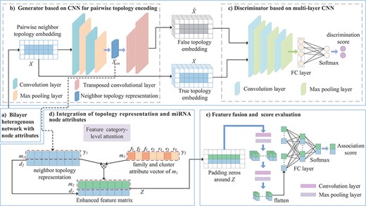
Framework of the proposed GMDA model. (A) Construction of bilayer heterogenous network with node attributes. (B) Generator based on CNN integrates the neighbor topology embedding of miRNA and disease nodes and produces neighbor topology representation. (C) Discriminator based on multi-layer CNN discriminates true topology embedding and the false one. (D) Integration of topology representation and miRNA node attributes to form enhanced feature matrix. (E) Final fusion and association score prediction.
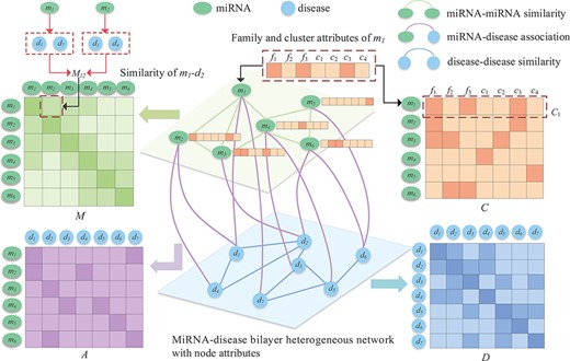
Bilayer heterogeneous network with node attributes composed of miRNA–miRNA similarity, miRNA–disease association and disease–disease similarity.
As shown in Figure 1, the model is composed of a generator, discriminator and convolution module. The adversarial learning between the generator and discriminator produces a neighbor topology representation of miRNA |${m_{i}}$| and disease |${d_{j}}$|, and the convolution neural network module with the attention mechanism integrates the neighbor topology representation of |${m_{i}}$| and |${d_{j}}$|, the node attribute representation of |${m_{i}}$| and the association prediction score of |${m_{i}}-{d_{j}}$| that is obtained through the fully connected layer and softmax layer.
2.3.1 GANs of miRNA–disease node pairs
The framework based on a GAN is mainly composed of a generator and discriminator. Given a pair of miRNAs and diseases, the main goal of the generator is to generate a false sample pair corresponding to the node pair as much as possible. The discriminator tries to distinguish the false sample pair from the true sample pair. The better trained the discriminator, the more helpful it is for the generator to generate more robust false sample pairs, which is iterative. In this iterative process, the performance of the generator and discriminator is significantly improved. The final discriminator can accurately distinguish true or false sample pairs, and the code part of the generator can produce a more robust low-dimensional neighbor topology representation of miRNA–disease pairs.
Construction of neighbor topology embedding matrix. The process of constructing the embedding matrix of the miRNA |${m_{1}}$| and disease |${d_{2}}$| node pairs is shown in Figure 3A. |${M_{1}}$| is the 1st row of the miRNA similarity matrix |$M$|, which represents the information of |${m_{1}}$| with all miRNA connected edges, and the weight of the edge is the similarity between |${m_{1}}$| and each miRNA. As shown in Figure 3A, |${m_{1}}$| has connected edges with |${m_{2}}$|, |${m_{3}}$| and |${m_{4}}$|, indicating that they have similar functions. The 1st row of the miRNA–disease association matrix |${A_{1}}$| represents the connections among |${m_{1}}$| and all diseases. A connection indicates that there is an association, and no connection denotes that it does not exist or that there is no association. We record the front and rear splices as the neighbor topology feature vector as |${x_{m_{1}}}$|. Similarly, |${A_{2}} ^{\mathrm{T}}$| and |${D_{2}}$| record the association-based and similar connection edges of |${d_{2}}$| with each miRNAs and diseases. The |${d_{2}}$| neighbor topology feature vector is formed by their front and rear splicing. Finally, |${x_{m_{1}}}$| and |${x_{d_{2}}}$| are stacked up and down to form the neighbor topology feature matrix |$X \in{\mathbb{R}^{2 \times{(N_{m} + N_{d})}}}$| of the node |${m_{1}}-{d_{2}}$| pairs. This representation is regarded as a true sample.
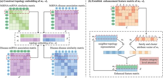
An illustration of the proposed construction of topology embedding and formation enhancement matrix between a pair of miRNA and disease. (A) Topology embedding matrix |$X$| of |${m_{1}}-{d_{2}}$| by embedding mechanism. (B) An attention mechanism at the feature category level combines the neighbor topology representation, family and cluster attributes of |$m_{1}$| to establish pairwise enhanced feature matrix.
Generator based on convolutional autoencoder. The generator generates the reconstructed neighbor topology matrix |$\hat{X}$| of the miRNA–disease node pair, which is regarded as a false sample. The main goal of the generator is to make the generated |$\hat{X}$| as close to |$X$| as possible. Given a node pair |${m_{i}}-{d_{j}}$|, the neighbor topology is embedded as |$X$|; the generator |$G(,;{\theta }_G)$| encodes it as shown in Figure 1.
For the discriminator to distinguish the possibility of a pair of true and false samples, there are two possible inputs as follows:
At the end of the optimization process, |${\left (X_{en}^{\left (N_{en}\right )}\right )}_1$| and |${\left (X_{en}^{\left (N_{en}\right )}\right )}_2$| are the 1st and 2nd rows of the matrix, respectively, and they are represented as neighbor topologies of the nodes |$m_i$| and |$d_j$|.
Results of ablation experiments on our method
| GAN | FC-attention | Average AUC | Average AUPR |
| ✗ | ✓ | 0.882 | 0.197 |
| ✓ | ✗ | 0.917 | 0.237 |
| ✓ | ✓ | 0.928 | 0.250 |
| GAN | FC-attention | Average AUC | Average AUPR |
| ✗ | ✓ | 0.882 | 0.197 |
| ✓ | ✗ | 0.917 | 0.237 |
| ✓ | ✓ | 0.928 | 0.250 |
The bold values indicate highest AUC and AUPR.
2.3.2 Attention mechanism at the feature category level
GMDA and other methods for the area under the ROC curve of all the diseases and 15 well-characterized diseases
| Disease name | AUC | |||||||
|---|---|---|---|---|---|---|---|---|
| GMDA | Liu’s method | PBMDA | DMPred | GSTRW | NCMCMDA | DBNMDA | AEMDA | |
| Average AUC on 341 diseases | 0.928 | 0.891 | 0.857 | 0.890 | 0.807 | 0.905 | 0.907 | 0.916 |
| Breast neoplasms | 0.991 | 0.920 | 0.906 | 0.974 | 0.837 | 0.983 | 0.982 | 0.990 |
| Hepatocellular carcinoma | 0.985 | 0.929 | 0.910 | 0.931 | 0.791 | 0.967 | 0.974 | 0.973 |
| Glioma | 0.957 | 0.914 | 0.882 | 0.835 | 0.786 | 0.928 | 0.940 | 0.944 |
| Acute myeloid leukmia | 0.948 | 0.910 | 0.885 | 0.963 | 0.796 | 0.937 | 0.968 | 0.920 |
| Lung neoplasma | 0.985 | 0.906 | 0.862 | 0.944 | 0.813 | 0.947 | 0.955 | 0.960 |
| Melanoma | 0.975 | 0.893 | 0.849 | 0.910 | 0.758 | 0.954 | 0.962 | 0.969 |
| Osteosarcoma | 0.967 | 0.897 | 0.860 | 0.985 | 0.771 | 0.968 | 0.961 | 0.987 |
| Ovarian neoplasms | 0.972 | 0.918 | 0.888 | 0.967 | 0.844 | 0.955 | 0.968 | 0.970 |
| Pancreatic neoplasms | 0.966 | 0.902 | 0.879 | 0.821 | 0.833 | 0.904 | 0.898 | 0.963 |
| Alzheimer disease | 0.925 | 0.875 | 0.833 | 0.922 | 0.816 | 0.897 | 0.901 | 0.924 |
| Carcinoma, renal cell | 0.946 | 0.900 | 0.856 | 0.791 | 0.786 | 0.935 | 0.799 | 0.956 |
| Diabetes mellitus, type 2 | 0.963 | 0.905 | 0.870 | 0.936 | 0.870 | 0.898 | 0.951 | 0.957 |
| Glioblastoma | 0.945 | 0.889 | 0.849 | 0.894 | 0.759 | 0.912 | 0.930 | 0.941 |
| Heart failure | 0.938 | 0.909 | 0.884 | 0.962 | 0.814 | 0.899 | 0.943 | 0.945 |
| Atherosclerosis | 0.929 | 0.911 | 0.891 | 0.955 | 0.824 | 0.961 | 0.959 | 0.924 |
The bold values indicate the highest AUCs.
GMDA and other methods for the area under the PR curve of all the diseases and 15 well-characterized diseases
| Disease name | AUPR | |||||||
|---|---|---|---|---|---|---|---|---|
| GMDA | Liu’s method | PBMDA | DMPred | GSTRW | NCMCMDA | DBNMDA | AEMDA | |
| Average AUPR on 341 diseases | 0.250 | 0.099 | 0.090 | 0.086 | 0.040 | 0.166 | 0.187 | 0.219 |
| Breast neoplasms | 0.915 | 0.725 | 0.718 | 0.800 | 0.389 | 0.812 | 0.821 | 0.903 |
| Hepatocellular carcinoma | 0.886 | 0.750 | 0.767 | 0.715 | 0.482 | 0.831 | 0.845 | 0.877 |
| Glioma | 0.439 | 0.436 | 0.390 | 0.175 | 0.225 | 0.312 | 0.210 | 0.427 |
| Acute myeloid leukmia | 0.332 | 0.41 | 0.385 | 0.466 | 0.123 | 0.358 | 0.369 | 0.478 |
| Lung neoplasma | 0.792 | 0.596 | 0.562 | 0.620 | 0.370 | 0.685 | 0.741 | 0.768 |
| Melanoma | 0.602 | 0.524 | 0.483 | 0.366 | 0.205 | 0.493 | 0.512 | 0.581 |
| Osteosarcoma | 0.499 | 0.374 | 0.357 | 0.620 | 0.180 | 0.486 | 0.604 | 0.621 |
| Ovarian neoplasms | 0.669 | 0.556 | 0.528 | 0.366 | 0.395 | 0.480 | 0.486 | 0.637 |
| Pancreatic neoplasms | 0.583 | 0.485 | 0.458 | 0.569 | 0.333 | 0.824 | 0.531 | 0.519 |
| Alzheimer disease | 0.235 | 0.143 | 0.136 | 0.351 | 0.086 | 0.218 | 0.359 | 0.361 |
| Carcinoma, renal cell | 0.341 | 0.354 | 0.314 | 0.206 | 0.136 | 0.254 | 0.293 | 0.322 |
| Diabetes mellitus, type 2 | 0.375 | 0.302 | 0.259 | 0.398 | 0.132 | 0.399 | 0.401 | 0.384 |
| Glioblastoma | 0.380 | 0.364 | 0.346 | 0.284 | 0.162 | 0.293 | 0.318 | 0.372 |
| Heart failure | 0.397 | 0.348 | 0.301 | 0.393 | 0.135 | 0.262 | 0.289 | 0.341 |
| Atherosclerosis | 0.276 | 0.298 | 0.306 | 0.309 | 0.084 | 0.289 | 0.310 | 0.287 |
The bold values indicate the highest AUPRs.
2.3.3 Predictive score evaluation based on convolution neural network
3 Experimental results and discussions
3.1 Parameter setting
In GMDA, the window sizes of |$3 \times 17$| and |$1 \times 2$| were applied to the convolution layer and the max-pooling layer, respectively. The transpose convolution used a window size of |$3 \times 18$|. The number of filters encoded in the generator was 30 and 60 in the 1st and 2nd layers, respectively. In contrast, the number of filters in the decoding part was 60 and 30 in the 1st and 2nd layers, respectively. During the process of association score evaluation, the sizes of filters within two convolutional layers were |$2\times 2$|. The numbers of filters were 40 and 20 in the 1st and 2nd layers, respectively. In the pooling layers, the window sizes of max pooling were |$2\times 2$|. We analyzed the time complexity of the GMDA. The corresponding analysis and the training time and testing time were listed in Supplementary Table 4. In addition, we evaluated the sensitivity coefficients [43] for GMDA’s parameters by changing one parameter and fixing the remaining ones. The number of the encoding layers |$L_{en}$| and of the decoding layers |$L_{de}$| was selected from {1, 2, 3}. For area under the receiver operating characteristic (ROC) curve (AUC), the sensitivity coefficient values of |$L_{en}$| and |$L_{de}$| were 0.04863 and 0.01790, respectively. In terms of area under the precision–recall (AUPR), the corresponding sensitivity coefficient values were 0.09905 and 0.07145. It indicates GMDA was not sensitive to the variations of |$L_{en}$| and |$L_{de}$| for the evaluation metric AUC, but they are a little sensitive to those of |$L_{en}$| and |$L_{de}$| for another metric AUPR. The experimental results were demonstrated in Supplementary Table 5. We used the Pytorch library to train and optimize the neural network parameters and used a GPU card (NVIDIA GeForce GTX 1080Ti) to speed up the training process.
3.2 Performance evaluation metrics
Five-fold cross-validation was performed to evaluate the performance of GMDA and the other models. All known miRNA–disease association data were partitioned into positive samples and randomly divided into five subsets. The same amount of unknown related data was randomly selected and divided into five negative subsets. In each fold, four positive and four negative subsets were used for training, and the remaining subsets were used for testing. The prediction scores of all test samples were arranged in descending order, such that the higher the ranking of positive samples, the better the performance of our model.
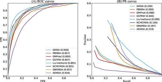
GMDA and other methods for the area under ROC and PR curves of all diseases.
AUC paired Wilcoxon test results of eight methods
| |$p$|-value between GMDA and other methods | Liu’s method | PBMDA | DMPred | GSTRW | NCMCMDA | DBNMDA | AEMDA |
|---|---|---|---|---|---|---|---|
| |$p$|-value of AUC | 4.2496e-41 | 9.8477e-32 | 7.3596e-37 | 6.5331e-20 | 6.3647e-22 | 5.6742e-18 | 3.1421e-12 |
| |$p$|-value of AUPR | 1.2063e-13 | 1.988e-22 | 6.5496e-8 | 1.4698e-15 | 3.0124e-16 | 2.1854e-10 | 1.7412e-11 |
Moreover, biologists often select the top candidate miRNAs in the predicted results for further biological experiments. Therefore, it is more attractive for biologists to have more positive samples in the order of the top |$k$| prediction results. We calculated the miRNA–disease pair recall rate of the top |$k$| candidates, i.e. the ratio of positive samples to all positive samples as another criterion to evaluate performance.
3.3 Ablation experiments
We performed ablation experiments to validate the contributions of major innovations including GAN and feature category-level attention (FC-attention). As shown in Table 1, GMDA that is the baseline with GAN and FC-attention achieved the best performance. Without GAN, AUC and AUPR dropped down by 4.6% and 5.3% when compared with baseline. The primary reason is GAN enhanced the feature representations of miRNA–disease node pairs which may improve the prediction performance. AUC and AUPR of the model without FC-attention mechanism decreased by 1.1% and 1.3%. It indicates that it is essential to deeply integrate the attributes of miRNA nodes.
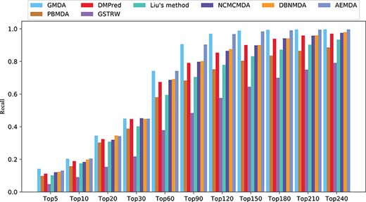
Recall rates of all diseases under different top |$k$|.
3.4 Comparison with other methods
GMDA was compared with state-of-the-art models for predicting disease-related miRNA candidates, including Liu’s method [13], PBMDA [12], DMPred [18], GSTRW [15], NCMCMDA [21], DBNMDA [32] and AEMDA [25]. To obtain the best performance, we set the super parameters to reach the value of their optimal performance described in the original paper. Our method and the compared methods are trained by using the same training dataset and testing dataset.
As shown in Figure 4A, GMDA achieved the highest average AUC (AUC=0.928+/-0.0041) among all 341 diseases tested. It exceeded Liu’s method by 3.7%, PBMDA by 7.1%, DMPred by 3.8%, GSTRW by 12.1%, NCMCMDA by 2.3%, DBNMDA by 2.1% and AEMDA by 1.2%. In addition, for the 15 well-characterized diseases, we listed the performances of these six methods. Because all these diseases have more than 80 associated miRNAs, the prediction results of these diseases could better reflect the performance of the model. The highest value of 10 diseases was obtained by GMDA among the AUCs of 15 diseases (Table 2).
As shown in Figure 4B, the value of GMDA under the average PR curve of 341 diseases was higher than that of the other models (AUPR = 0.250+/-0.0036). Its average performance exceeded that of Liu’s method, PBMDA, DMPred, GSTRW, NCMCMDA, DBNMDA and AEMDA by 15.1%, 16%, 16.4%, 21%, 8.4%, 6.3% and 3.1%, respectively. Among the 15 well-characterized diseases, GMDA achieved the highest value of 10 (Table 3).
Both the AUC and AUPR of GMDA achieved the best performance because our prediction model, based on GANs, could deeply integrate the neighbor topology of miRNA and disease node pairs, the attribute information of the miRNA family and cluster. AEMDA achieved the 2nd-best performance (AUC = 0.916). It adopted a fully connected autoencoder to infer the potential associations between miRNAs and diseases. DBNMDA achieved the 3rd-best performance (AUC = 0.907). The prediction algorithm of this method was based on a deep belief network and was subordinate to a class of deep learning algorithms. This indicated deep learning-based algorithms can deeply integrate the complex relationships between miRNA and disease-related associations. Hence, it is helpful to construct a deep learning-based algorithm. Both the AUC and AUPR of NCMCMDA were higher than those of Liu’s method, PBMDA, DMPred and GSTRW. The AUPR of Liu’s method was slightly higher than that of PBMDA, but its AUC was 3.4% higher than that of PBMDA. The AUPR of DMPred was slightly lower than that of PBMDA, but its AUC is higher than PBMDA. The AUC and AUPR of GSTRW were not as high as those of other methods. The main reason was that it only uses the similarity of diseases and miRNA and does not consider the important correlation information between them. This confirmed that it is necessary to make full use of the multiple connections between miRNAs and diseases.
To further verify whether GMDA’s performance was significantly better than that of the others, we conducted a paired Wilcoxon test on 341 diseases. As shown in Table 4, the |$p$|-value values of GMDA in terms of both AUC and AUPR were less than 0.05. This statistical result showed that its performance was significantly better than that of the other methods.
In addition, the higher the recall rate of the top |$k$| miRNAs and disease-related candidates, the more disease-related miRNAs could be correctly identified. The average recall rates of the eight methods in the top |$k$| candidates among the 341 diseases are shown in Figure 5. Under different threshold |$k$|, the recall rates of GMDA were better than those of the other methods. It ranked 20.3% of the positive samples in the top 10, 45% in the top 30, 74.2% in the top 60 and 90.6% in the top 90. AEMDA achieved the decent recall rates, which ranked 20.5%, 44.9%, 74.2% and 90.4% in the top 10, 30, 60 and 90. The recall rates of DMPred were very close to those of DBNMDA. The former ranked 18.9%, 44.7%, 67.4% and 79.1% in the top 10, 30, 60 and 90. The latter was slightly higher than the former, and it ranked 19.9%, 44.8%, 69.1% and 80.2%. NCMCMDA ranked 18.4%, 45.2%, 68.7% and 79.8%. The recall rates of Liu’s method were higher than those of PBMDA. The former ranked 17.5%, 40.2%, 59.5%, 70.5% and the latter ranked 15.8%, 38.8%, 58.1%, 68.3% in the top 10, 30, 60, 90, respectively. The recall rates of GSTRW were still not as high as those of the other methods, and its corresponding recall rates were 10.1%, 21.8%, 37.9% and 48.4%.
3.5 Case studies: lung neoplasms, breast neoplasms and pancreatic neoplasms
To further confirm that GMDA can detect high-quality potential disease-related candidate miRNAs, we performed case studies on lung tumors, breast tumors and pancreatic tumors. We used lung tumor as an example, and the results of the top 50 candidate miRNAs are given in Table 5. In addition, we listed the top 50 candidates for breast and pancreatic tumors in Supplementary Tables 1 and 2, respectively.
The top 50 miRNA candidates related to lung neoplasms
| Rank | MiRNA name | Evidence | Rank | MiRNA name | Evidence |
|---|---|---|---|---|---|
| 1 | hsa-mir-614 | dbDEMC,miRCancer | 26 | hsa-mir-608 | dbDEMC |
| 2 | hsa-mir-610 | dbDEMC,miRCancer | 27 | hsa-mir-199a | dbDEMC,PhenomiR |
| 3 | hsa-mir-203b | dbDEMC | 28 | hsa-mir-22 | dbDEMC,PhenomiR,miRCancer |
| 4 | hsa-mir-216b | dbDEMC,miRCancer | 29 | hsa-mir-376a | dbDEMC,PhenomiR,miRCancer |
| 5 | hsa-mir-378d | dbDEMC | 30 | hsa-mir-708 | dbDEMC,miRCancer |
| 6 | hsa-mir-137 | dbDEMC,PhenomiR,miRCancer | 31 | hsa-mir-410 | dbDEMC,miRCancer |
| 7 | hsa-mir-574 | dbDEMC,PhenomiR | 32 | hsa-mir-223 | dbDEMC,PhenomiR,miRCancer |
| 8 | hsa-mir-517a | dbDEMC | 33 | hsa-mir-219 | dbDEMC,PhenomiR,miRCancer |
| 9 | hsa-mir-190b | dbDEMC | 34 | hsa-mir-148a | dbDEMC,PhenomiR,miRCancer |
| 10 | hsa-mir-23b | dbDEMC,PhenomiR,miRCancer | 35 | hsa-mir-203 | dbDEMC,PhenomiR,miRCancer |
| 11 | hsa-mir-32 | dbDEMC,PhenomiR,miRCancer | 36 | hsa-mir-361 | dbDEMC,PhenomiR,miRCancer |
| 12 | hsa-mir-187 | dbDEMC,PhenomiR,miRCancer | 37 | hsa-mir-19 | Literature [48] |
| 13 | hsa-mir-10b | dbDEMC,PhenomiR,miRCancer | 38 | hsa-mir-374a | dbDEMC,PhenomiR,miRCancer |
| 14 | hsa-mir-29a | dbDEMC,PhenomiR,miRCancer | 39 | hsa-mir-106b | dbDEMC,PhenomiR,miRCancer |
| 15 | hsa-mir-500 | dbDEMC | 40 | hsa-mir-302a | dbDEMC,PhenomiR,miRCancer |
| 16 | hsa-mir-15b | dbDEMC,PhenomiR,miRCancer | 41 | hsa-mir-30d | dbDEMC,PhenomiR,miRCancer |
| 17 | hsa-mir-663 | dbDEMC,miRCancer | 42 | hsa-mir-15a | dbDEMC,PhenomiR,miRCancer |
| 18 | hsa-mir-93 | dbDEMC,PhenomiR,miRCancer | 43 | hsa-mir-208a | dbDEMC,PhenomiR,miRCancer |
| 19 | hsa-mir-27b | dbDEMC,PhenomiR,miRCancer | 44 | hsa-mir-30b | dbDEMC,PhenomiR,miRCancer |
| 20 | hsa-mir-96 | dbDEMC,PhenomiR,miRCancer | 45 | hsa-mir-222 | dbDEMC,PhenomiR,miRCancer |
| 21 | hsa-mir-33b | dbDEMC,miRCancer | 46 | hsa-mir-302c | dbDEMC,PhenomiR |
| 22 | hsa-mir-429 | dbDEMC,miRCancer | 47 | hsa-mir-326 | dbDEMC,PhenomiR,miRCancer |
| 23 | hsa-mir-140 | dbDEMC,PhenomiR,miRCancer | 48 | hsa-mir-381 | dbDEMC,PhenomiR,miRCancer |
| 24 | hsa-mir-127 | dbDEMC,PhenomiR,miRCancer | 49 | hsa-mir-20b | dbDEMC,PhenomiR |
| 25 | hsa-mir-720 | dbDEMC | 50 | hsa-mir-141 | dbDEMC,PhenomiR,miRCancer |
First, text mining techniques described by Xie |$et$||$al.$| [45] to extract experimentally validated associations between miRNAs and cancers were used. The associations were further verified manually and included in the miRCancer database, which contained 9080 miRNA–disease associations, covering 57984 miRNAs and 196 cancers. As shown in Table 5, miRCancer included 38 candidates, indicating that these miRNAs were associated with regulatory disorders in lung tumors and that these candidates were associated with the disease. Second, dbDEMC [46] is an integrated miRNA database designed to show the differential expression of miRNAs in human cancers. The database covers 2224 miRNAs and 36 cancer types. Similarly, the PhenomiR [47] database provides information about differentially regulated miRNA expression in diseases and other biological processes. dbDEMC includes 49 candidate miRNAs and PhenomiR includes 34 candidates, which indicated that their expression is upregulated or downregulated in lung cancer tissues. One candidate miRNA labeled ‘literature’ was supported by the published literature. Compared with normal tissues, the expression of these three miRNAs in lung tumors was confirmed to be dysregulative [48].
Among the 50 candidate miRNAs for breast tumors (Supplementary Table 1), 33 candidates were recorded by miRCancer, which indicated that they were indeed associated with diseases. PhenomiR and dbDEMC included 25 and 49 candidate miRNAs, respectively, indicating that there was a significant difference in their expression between normal tissues and breast tumors. Supplementary Table 2 records the top 50 candidate miRNAs, for pancreatic tumors, of which miRCancer contained 24 candidates, and 45 and 30 candidate miRNAs were recorded by dbDEMC and PhenomiR, respectively. One candidate supported in the literature was abnormally expressed in pancreatic tumor tissues.
3.6 Prediction of novel miRNAs related to diseases
After the prediction model is trained by using all the miRNA–disease associations, we applied it to predict candidate miRNAs for each disease. We randomly selected the unobserved miRNA–disease association pairs (negative samples) whose size is equal to that of known miRNA–disease associations (positive samples) to train the model. The top-ranked 50 candidate miRNAs are listed in the Supplementary Table 3, which may help the biologists identify actual miRNA–disease associations by wet laboratory experiments.
4 Conclusions
We proposed a GMDA model which learns from a bilayer heterogeneous network to predict potential miRNA–disease associations. This model captured the similarities between miRNA and disease nodes and, more importantly, the intra-relations in terms of known miRNAs and diseases associations, family and cluster information related to miRNA nodes. The generator based on convolutional autoencoder and the discriminator based on multi-layer CNN learned and integrated neighbor topology representation and miRNA node attribute representation. The novel feature category level attention mechanism assigned different weights to the two types of miRNA features for adaptively fusion. Comparison results with state-of-the-art methods demonstrated the improved performance for miRNA–disease association prediction. Case studies on three cancers further confirmed our model’s ability in identifying potential candidate disease-related miRNAs. GMDA can be used as a prioritization tool to generate reliable candidates for facilitating biological wet laboratory experiments to identify real associations between miRNAs and diseases.
|$\bullet $| A bilayer heterogeneous network with node attributes is constructed, which benefits the extraction and representation of miRNAs and diseases relations, as well as the family and cluster attributes of miRNA nodes.
|$\bullet $| Novel pairwise neighbor topology representation to reveal the common neighbors of miRNA and disease; a module based on generative and adversarial network to enhance the pairwise neighbor topology learning.
|$\bullet $| Newly proposed node attributes of an miRNA show the families and clusters to which the miRNA belongs. A newly proposed attention mechanism at feature category level to distinguish the importance of different features of miRNA nodes for weighted fusion.
|$\bullet $| Improved predictive performance confirmed by comprehensive evaluations, including comparison with five state-of-the-art models on public dataset, a paired Wilcoxon test, recall rates on 341 diseases and case studies of three cancers.
Funding
Natural Science Foundation of China (61972135, 62172143); Natural Science Foundation of Heilongjiang Province (LH2019F049 and LH2019A029); China Postdoctoral Science Foundation (2019M650069, 2020M670939); Heilongjiang Postdoctoral Scientific Research Staring Foundation (BHLQ18104); Fundamental Research Foundation of Universities in Heilongjiang Province for Technology Innovation (KJCX201805); Innovation Talents Project of Harbin Science and Technology Bureau (2017RAQXJ094); Fundamental Research Foundation of Universities in Heilongjiang Province for Youth Innovation Team (RCYJTD201805); Foundation of Graduate Innovative Research (YJSCX2021-199HLJU).
Ping Xuan, PhD (Harbin Institute of Technology), is a professor at the School of Computer Science and Technology, Heilongjiang University, Harbin, China. Her current research interests include computational biology, complex network analysis and medical image analysis.
Dong Wang is studying for his master’s degree in the School of Computer Science and Technology at Heilongjiang University, Harbin, China. His research interests include complex network analysis and deep learning.
Hui Cui, PhD (The University of Sydney), is a lecturer at Department of Computer Science and Information Technology, La Trobe University, Melbourne, Australia. Her research interests lie in data-driven and computerized models for biomedical and health informatics.
Tiangang Zhang, PhD (The University of Tokyo), is an associate professor of the School of Mathematical Science, Heilongjiang University, Harbin, China. His current research interests include complex network analysis and computational fluid dynamics.
Toshiya Nakaguchi, PhD (Sophia University), is a professor at the Center for Frontier Medical Engineering, Chiba University, Chiba, Japan. His current research interests include medical image processing, machine learning, image-guided surgery and biomedical measurement.
References
Matsuyama H, Suzuki HI.
Chen X, Wu QF, Yan GY, et al.
Li A, Deng YW, Tan Y, et al.
Xuan P, Shen TH, Wang X, et al.
Chen X, Li TH, Zhao Y, et al.
Stark VA, Facey COB, Viswanathan V, et al.
Nair V, Hinton GE.
