


Abstract
Identifying and characterizing the interaction between risk factors for multiple outcomes (multi-outcome interaction) has been one of the greatest challenges faced by complex multifactorial diseases. However, the existing approaches have several limitations in identifying the multi-outcome interaction. To address this issue, we proposed a multi-outcome interaction identification approach called MOAI. MOAI was motivated by the limitations of estimating the interaction simultaneously occurring in multi-outcomes and by the success of Pareto set filter operator for identifying multi-outcome interaction. MOAI permits the identification for the interaction of multiple outcomes and is applicable in population-based study designs. Our experimental results exhibited that the existing approaches are not effectively used to identify the multi-outcome interaction, whereas MOAI obviously exhibited superior performance in identifying multi-outcome interaction. We applied MOAI to identify the interaction between risk factors for colorectal cancer (CRC) in both metastases and mortality prognostic outcomes. An interaction between vaspin and carcinoembryonic antigen (CEA) was found, and the interaction indicated that patients with CRC characterized by higher vaspin (≥30%) and CEA (≥5) levels could simultaneously increase both metastases and mortality risk. The immunostaining evidence revealed that determined multi-outcome interaction could effectively identify the difference between non-metastases/survived and metastases/deceased patients, which offers multi-prognostic outcome risk estimation for CRC. To our knowledge, this is the first report of a multi-outcome interaction associated with a complex multifactorial disease. MOAI is freely available at https://sites.google.com/view/moaitool/home.
Introduction
The interaction between risk factors (e.g. polymorphism and the environment) is mainly due to the marginal effects of multiple risk factors showing different deviations, which could become the key to affect disease [1]. The degree of the marginal effect represents the marginal distribution of factors with each other. If the risk factor has no marginal effect, it means that there is no difference between the case and control groups, whereas the difference between the case and control groups could gradually become apparent when the marginal effect of the factor is increased [2]. However, a single risk factor could have a weaker marginal effect among the interactions between risk factors [3]. These risk factors with weaker marginal effects could be filtered when typical feature selection methods are used. When these risk factors appear together, the interaction between risk factors with the formation of disease phenotypes can be found [4]. Furthermore, the interaction between risk factors could have a synergistic or additive effect on the multi-outcome (e.g. multiple disease phenotypes) [5–7]. The multi-outcome interaction might explain differences in disease risk and effect on the multiple disease pathogenesis [8]. However, many studies consider only a single single-outcome (disease phenotype) to identify the interaction between risk factors [1, 9], thereby ignoring the interaction effects on others outcome (disease phenotypes).
Parametric statistical methods generate models of the relationships between discrete predictors that are completely or partially dependent on interactions with polymorphisms [10] and interactions with environmental exposures in the discrete clinical outcomes [11]. Cox proportional hazard (CoxPH) regression is essentially a robust regression model for mortality analysis, which is often used to investigate the associations between interest characteristics and hazard time of observed patients [12]. CoxPH regression is a parametric statistical model which is highly dependent on the sample distribution, and a wide confidence interval (CI) presented in the CoxPH model indicates that the findings are less certain. Therefore, the use of CoxPH regression is not feasible in the investigation of the interaction using small samples [13]. In addition, parametric statistical methods are less practical for processing high-dimensional data, which might model multi-order interactions that contain many empty cells in the contingency table cells, leading to very large coefficient estimates and standard errors [14]. Unlike parametric statistical methods, machine learning (ML) has nonparametric (distribution-free) and model-free (it assumes no particular inheritance model) characteristics. Multifactor dimensionality reduction (MDR) is an ML method and is proposed for identifying interactions between risk factors [3]. MDR uses a data reduction process to categorize the dimensionality of multiple factors into high- and low-risk groups. This reduction process enables the transformation of high-dimensional multifactors into a two-way contingency table. Therefore, the scheme of the data reduction process can effectively address the limitation of parametric statistical methods. Many improved MDR methods have been proposed to enhance the MDR quality of interaction identification, including the BMDR [15], MDR-LR [8], MDR-NMI [16] and MCDA-MDR [17]. However, these methods are still impossible to consider the interaction between risk factors of multiple outcomes (multi-outcome interaction). Consequently, the interaction between risk factors of multi-outcome identification is still a vital challenge. One solution to this challenge is to identify the interaction between risk factors in each outcome. After identifying the interactions in all outcomes, the optimal solution is selected when the interaction appears in all outcomes. An alternative solution is to develop new statistical and computational methods to identify multi-outcome interaction. To address this issue, we proposed a multi-outcome interaction identification approach called MOAI. We first evaluate the MOAI by using simulated high-dimensional multi-outcome data with epistatic effects, and we then used MOAI to identify the multi-outcome interaction between multiple risk factors associated with colorectal cancer (CRC).
CRC is a heterogeneous malignant tumor with unfavorable prognostic mortality outcomes [18]. Therefore, prognostic factors for CRC have become an important research field in cancer studies. The progression of CRC is currently thought to be a complicated, multistep process involving multifactor regulation [19]. Despite early detection and therapeutic advances, disease progression, including lymphatic and distant metastases, remains to be the major cause of death in patients with CRC, and the mortality of advanced CRC remains unsatisfactory [19]. Therefore, a thorough understanding of CRC molecular pathogenesis may benefit the discovery of prognostic markers for patients [20]. The carcinoembryonic antigen (CEA) is reported as a biomarker for cancer prognosis in CRC [21–23]. Previous studies have demonstrated that the CEA levels could be considered as independent prognostic factors in CRC [24–26]. A visceral adipose tissue-derived serine protease inhibitor, known as vaspin, is one of the identifying adipokines and has been shown to have an impact on several different types of cancer [27, 28]. Vaspin levels have been reported as a potential biomarker in the carcinogenesis of medullary thyroid carcinoma [28]. Furthermore, a previous study has reported that the vaspin expression level is relatively higher in CRC, which might be due to the potential relationship between adipocytokines and the development of CRC [29]. The above-mentioned risk factors have been determined for their associations related to the CRC on the multiple prognostic outcomes, including metastasis and mortality. However, the interaction between risk factors related to CRC on the metastasis and mortality outcomes is seldom reported.
We hypothesize that multi-outcome interactions between risk factors may have a synergistic or additive effect on the prognosis of CRC. Application of MOAI to a CRC multi-outcome case–control data set, in the absence of any statistically significant independent main effects, identified a statistically significant multi-outcome interaction among risk factors associated with CRC—tumor stage, grade, gender, age at diagnosis, body mass index (BMI), diabetes mellitus (DM), vascular invasion, perineurial invasion and serum CEA level. The immunostaining evidence revealed that multi-outcome interaction could effectively identify the difference between non-metastases/survived and metastases/deceased patients, which offer multi-prognostic outcome risk estimation for CRC.
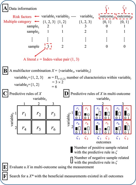
Diagram of the multi-outcome interaction identification problem. (A) Data information, (B) Multifactor combination, (C) Predictive rules, (D) Predictive rules in multi-outcome, (E) Evaluation of multifactor combination in multi-outcome, and (F) Determination of best multifactor combination in multi-outcome.
Materials and methods
Multi-outcome interaction identification problem
The purpose of the multi-outcome interaction identification problem is to identify an interaction between multiple variables (≥2 risk factors) related to multi-outcome (≥2 outcomes) (Figure 1). A variable includes the multiple characteristics denoted as {1, 2, …} [11] (Figure 1A). A sample includes multiple variables and multi-outcome in the data set. A literal s is defined as an index-value pair (i, v), with i denoting an index and v denoting a characteristic in a variable. In the present study, we focus on two-order interactions (i.e. the interaction between two variables) and two outcomes. A predictive rule in multi-outcome is an interaction between the variables in multi-outcome, which is defined as an interaction containing conjunctive rules (r, ζk): si∩sj → ζk, where i ≠ j, implying an interaction between a conjunction of two literals (si, sj) denoted as r, and ζk is the multi-outcome (k = {1, 2}, ζk = 1 represents the positive and ζk = 0 represents the negative). A multifactor combination X between two variables contains M predictive rules (r1, r2, …, rM), where M is the number of combinations between two variables Si and Sj (i ≠ j), ∀r ∈ Si∪Sj (Figure 1B–D). The multi-outcome interaction identification problem is performed by searching for an X with the beneficial measurements (Figure 1E and F) in all outcomes.
MOAI
A novel algorithm for multi-outcome interaction identification problem, called MOAI, was proposed in the present study. MOAI was inspired by MDR [3], SNPRuler [4] and MCDA-MDR [17]. MOAI evaluated the interaction between two variables via highlighting the explanatory variables combination for multi-outcome according to the proportion difference in binary characteristics. M predictive rules within an interaction in multi-outcome were categorized into either predicted positive or negative groups (i.e. explanatory variable). Therefore, in multi-outcome, MOAI can determine whether there is a significant interaction between the response variable (positive/negative groups) and explanatory variable (predicted positive/negative groups) in a two-way contingency table. Strategic dominance is used to compare two multifactor combinations to determine which one is better with respect to measurement. A multifactor combination X1, which is not dominated by any multifactor combination X, is regarded as a candidate and is added into a Pareto set. MOAI used the cross-validation (CV) to avoid the overfitting of training data and the reducing of false positives in the statistical analysis. The 5-fold CV is used to repeat the process of identifying candidates five times. Consequently, five Pareto sets can be obtained. Finally, MOAI pools all candidates from five Pareto sets and counts the number of occurrences of each candidate; the multifactor combinations with the highest number of occurrences are outputted as optimal multi-outcome interactions. The diagram of MOAI is represented in Figure 2. MOAI includes the following eight steps:
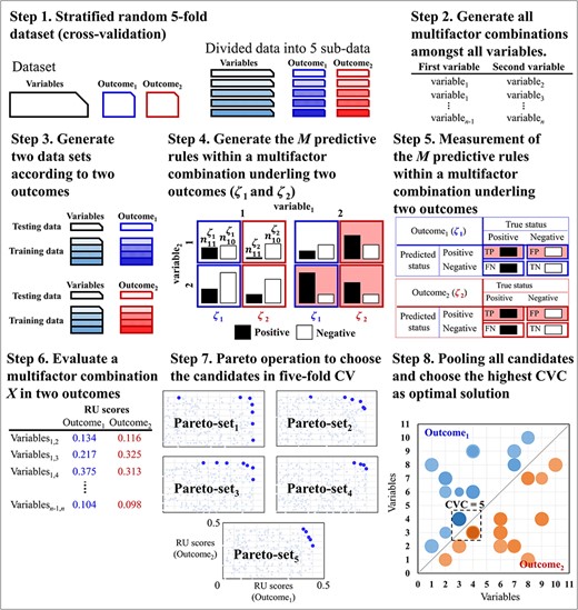
Schematic of the MOAI procedure. In steps 1–6, the blue and red colors indicate outcome1 and outcome2, respectively. In step 7, the points with light colors are the two RU scores of all interactions, and the points with dark colors are the two RU scores of the selected candidates in the kth Pareto set. In step 8, the size of the bubble is the average of the RU scores of the Pareto sets containing the specific interaction. The dark color indicates higher CVC.
Step 1: The data set is divided into five sub-data for a 5-fold CV. For a process in a 5-fold CV, one sub-data are used as the testing data, and the remaining four sub-data are used as training data. The process uses the training data to determine the candidate set (i.e. a set of multifactor combinations) throughout the six steps as following steps 2–7, and the relevant testing data are used to assess the quality of a multifactor combination X in the candidate set. In step 1, five Pareto sets are generated in an empty space, and a Pareto set is relevant to the process in a 5-fold CV.
Step 2: Generate all two-order multifactor combinations among all variables. The set consisted of all two-order multifactor combinations between two variables generated from all variables.
Step 3: Generate two data sets according to two outcomes. In the kth-fold CV, where k = {1, 2, …, 5} is the number of the process being executed in the 5-fold CV, the training and testing sub-data are copied into two data sets. The first data set includes the first outcome information (ζ1), and the second data set includes the second outcome information (ζ2).
Step 4: Generate the M predictive rules within a multifactor combination X underling two outcomes, i.e. M = μi × μj, where i ≠ j, μi and μj are the number of characteristics within the ith and jth variables, respectively. In the mth predictive rule, |${n}_{m1}^{\zeta }$| and |${n}_{m0}^{\zeta }$|are, respectively, the display of counts for the positive and negative within a ζ outcome, where ζ = {ζ1, ζ2} and m = {1, 2, …, M}. Counts for the positive and negative within the ζ1 outcome use the first data set of step 3, and counts for the positive and negative within the ζ2 outcome use the second data set of step 3.
Step 5: Measurement of the M predictive rules within a multifactor combination X.
Step 5.2: Each predictive rule is categorized into either predicted positive (|$\overline{P}$|) or predicted negative (|$\overline{N}$|). The mth predictive rule is categorized to |$\overline{P}$| if |${\theta}_m^{\zeta }$|≥1 [3]; otherwise, the mth predictive rule is categorized to |$\overline{N}$|, where m = {1, 2, …, M}.
Higher U(X, ζ) scores indicate stronger interactions between risk factors.
Step 7: Pareto set filter operator to choose the candidates. Two RU scores of a multifactor combination X in two outcomes (i.e. U(X, ζ1) and U(X, ζ2)) can be calculated from step 6. Pareto set filter operator selects the candidates with high RU scores by strategic dominance. The strategic dominance compares the two RU scores of a multifactor combination X with another multifactor combination X′ to determine which one is better. Pareto set filter operator involves two steps.
Step 7.1: A multifactor combination X is compared with all candidates in the kth Pareto set, where k = {1, 2, …, 5} is the number of the process being executed in 5-fold CV; if the kth Pareto set is empty, X is added to the kth Pareto set; if X is not dominated by any candidate, go to step 7.2; otherwise, start to perform the next evaluation of interaction (i.e. step 3).
Step 7.2: A multifactor combination X is compared with all candidates in the kth Pareto set; if a multifactor combination X dominates X′, X′ is discarded from the kth Pareto set. An interaction X is regarded as a candidate and is added to the kth Pareto set when all candidates are compared. All candidates are collected in the kth Pareto set. After evaluating all multifactor combinations within a process in kth-fold CV, the next sub-data are used as the testing data, and the remaining four sub-data are used as the training data, and we should perform steps 2–7 until all processes in a 5-fold CV are completed. Consequently, the five Pareto sets can be obtained.
Step 8: Pooling all candidates from five Pareto sets and counting the number of occurrences of each candidate (i.e. a multifactor combination). In the pooling, an occurrence frequency of a multifactor combination X in a 5-fold CV is counted, which is known as the CVC. A multifactor combination X with the highest CVC is determined as an interaction; if many multifactor combinations occur equally frequently of occurrences, these multifactor combinations are determined as the interactions (step 8 of Figure 2).
Statistical analysis
Statistical analysis is introduced in supplementary file.
Real-world data sources
Cancer tissue samples and analyzed data from 89 patients with surgically treated CRC diagnosed between January 2006 and December 2007 were collected at Kaohsiung Medical University Hospital under the approved protocol (KMUH-IRB-20130167). The median follow-up interval of the CRC study population was 66 (22–84) months. The 34 metastases and 46 mortality events were observed during the study period, and 38 patients were censored. All baseline characteristics were retrospectively collected from medical records. Baseline characteristics, including age at diagnosis, gender, BMI, DM, tumor stage, grade, lymph node invasion, vascular invasion, perineurial invasion, serum CEA and serum vaspin level, were included (Table 1). Tumor staging was performed according to the American Joint Committee on Cancer tumor-node-metastasis staging system [30], and the histological grade was classified according to the World Health Organization histological criteria [31]. Metastasis was defined as the patient who had distant metastasis within the follow-up interval, and the survival interval was calculated from the date of surgery until the date of first distant metastasis. Mortality was defined as patients dying during the follow-up interval, and the survival interval was calculated from the date of surgery until the date of death. Patients with no metastases who died within the follow-up interval were tracked from the date of surgery until the end of the study.
Baseline characteristics of study population (N = 89); P-value estimated using chi-squared or Fisher’s exact test
| Factors | Total | Metastases (n = 34) | P-value | Mortality (n = 46) | P-value |
|---|---|---|---|---|---|
| Age ≥ 65 years | 43 (48.3%) | 28 (44.1%) | 0.686 | 14 (63.0%) | 0.008 |
| Male | 59 (66.3%) | 34 (73.5%) | 0.366 | 25 (73.9%) | 0.177 |
| BMI ≥ 24 | 35 (39.3%) | 18 (50.0%) | 0.162 | 19 (34.8%) | 0.490 |
| DM | 28 (31.5%) | 15 (38.2%) | 0.397 | 10 (39.1%) | 0.167 |
| Stages III and IV | 44 (49.4%) | 18 (76.5%) | <0.001 | 15 (63.0%) | 0.015 |
| Grade III | 8 (9.0%) | 6 (5.9%) | 0.671 | 3 (10.9%) | 0.787 |
| N1-2 | 41 (46.1%) | 18 (67.6%) | 0.002 | 15 (56.5%) | 0.067 |
| Vascular invasion | 43 (48.3%) | 20 (67.6%) | 0.008 | 16 (58.7%) | 0.070 |
| Perineurial invasion | 55 (61.8%) | 28 (79.4%) | 0.013 | 20 (76.1%) | 0.008 |
| CEA ≥ 5 | 47 (52.8%) | 26 (76.5%) | <0.001 | 34 (73.9%) | <0.001 |
| Vaspin ≥ 30% | 43 (48.3%) | 24 (70.6%) | 0.002 | 34 (73.9%) | <0.001 |
Bold type indicates the significant difference (P-value < 0.05).
Immunohistochemistry (IHC)
IHC is introduced in supplementary file.
Evaluation of immunohistochemical staining
Evaluation of immunohistochemical staining is introduced in supplementary file.
Results
Simulation experiments
Disease models with marginal effect and without marginal effect were used to simulate the interaction between two variables for evaluating the algorithm performance for multi-outcome interaction identification. GAMETES [32] tool was used to randomly generate a data set consisting of 1000 variables (disease loci) in which a specific variable pair (objective variable1 and variable2) was generated according to the multilocus penetrances of the disease model, and other variables were generated with both minor allele frequencies (MAFs) and heritability (h2) values (Figure 3). The MAFs and h2 values affect the phenotypic variation to generate the different interaction structures. Data sets are then sorted according to the characteristic combination of objective variable1 and variable2. In each characteristic combination, the zeros (i.e. positive group) and ones (i.e. negative group) in the original outcome were, respectively, counted. A new outcome2 containing zeros and ones was randomly generated according to the frequencies of zeros and ones in the original outcome. Therefore, outcome2 has the same disease model setting as the original outcome, but the values of outcome2 and the original outcome may not be the same in a sample. In each disease model, 100 data sets were randomly generated by the above approach. The BMDR (2020) [15], MDR-LR (2018) [8], MDR-NMI (2019) [16], SNPRuler (2010) [4] and MCDA-MDR (2019) [17] were used to compare the MOAI with respect to the performance of two outcome interaction identification. MOAI can directly identify a specific variable pair (goal detection) in two outcomes. Other five algorithms need to identify a data set based on the original outcome (outcome1) and a data set based on generated outcome (i.e. outcome2). A goal detection of the five algorithms indicates that a specific variable pair is successfully identified in both two data sets based on outcome1 and outcome2. Identification success rates can be calculated by observing the frequency of goal detection within a specific variable pair (objective variable1 and variable2) for each of the 100 data sets.
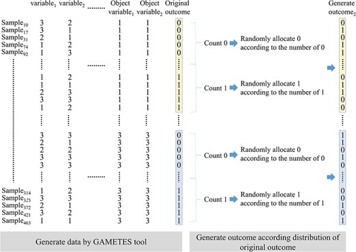
Diagram of a simulated data set.
Comparison of six algorithms in disease models with marginal effects
Parameter settings of multilocus penetrances, h2 and MAFs of six disease models with marginal effects were obtained from the existing literature [33, 34] and are shown in Supplementary Table S1 available online at http://bib.oxfordjournals.org/. In each disease model, the process of simulating 100 data sets based on the parameter settings of a disease model was introduced in the Simulation experiments section. A success rate of specific variable pair identification (identification success rate) with a disease model in 100 data sets is successfully calculated according to the solutions identified by an algorithm. Each correct identification belongs to a particular CVC (i.e. CVC = 1, 2, …, 5) as calculated. Therefore, the number of correct identifications in each CVC can be calculated.
Comparison of identification success rates of six algorithms is shown in Figure 4. For CVC = 2–5 (gray and black bars), the identification success rates of MDR-LR were close to MDR-NMI and MCDA-MDR in six models. BMDR can only identify the disease models 1 and 4, and the identification success rates were 16 and 28, respectively. MOAI has superior identification success rates than MCDA-MDR, SNPRuler, MDR-NMI, MDR-LR and BMDR. The CVC = 5 (Figure 4; black bar) indicates that the algorithm strongly determines an interaction X as a multi-outcome interaction. The results of CVC = 5 demonstrated that MOAI outperforms the other five algorithms. The Wilcoxon signed-rank test was used to evaluate the difference between MOAI and other algorithms. In Table 2, a significant difference between MOAI and another algorithm was determined when the P-value was <0.05. R+ is the number of times when MOAI outperformed another algorithm in six disease models with marginal effects. R− is the number of times when MOAI performed less than another algorithm in six disease models with marginal effects. R= is the number of times when MOAI had the same performance with another algorithm in six disease models with marginal effects. MOAI exhibited the highest R+, and all P-values were <0.05 in both CVC = 2–5 and CVC = 5 of six models with marginal effects. The results demonstrated that MOAI could effectively identify multi-outcome interaction in disease models with marginal effects.
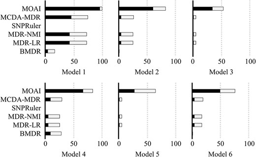
Comparison of MCDA-MDR, SNPRuler, MDR-NMI, MDR-LR, BMDR and MOAI when disease models with marginal effects were used. The bars represent the identification success rate, the black areas represent the correct identification with CVC = 5 and the gray areas represent the correct identification with CVC = 2–4.
Comparison of MCDA-MDR, SNPRuler, MDR-NMI, MDR-LR, BMDR and MOAI in disease models with marginal effects using the Wilcoxon signed-rank test
| MOAI versus | R− | R+ | R= | P-value |
|---|---|---|---|---|
| CVC = 2–5 | ||||
| MCDA-MDR | 0 | 6 | 0 | 0.028 |
| SNPRuler | 0 | 6 | 0 | 0.028 |
| MDR-NMI | 0 | 6 | 0 | 0.028 |
| MDR-LR | 0 | 6 | 0 | 0.028 |
| BMDR | 0 | 6 | 0 | 0.028 |
| CVC = 5 | ||||
| MCDA-MDR | 0 | 6 | 0 | 0.028 |
| SNPRuler | 0 | 6 | 0 | 0.028 |
| MDR-NMI | 0 | 6 | 0 | 0.028 |
| MDR-LR | 0 | 6 | 0 | 0.028 |
| BMDR | 0 | 6 | 0 | 0.028 |
R−, negative ranks; R+, positive ranks; R=, ties, bold value indicates the significant improvement (P-value < 0.05).
Comparison of six algorithms in disease models without marginal effects
Details of multilocus penetrances, h2 and MAFs of 30 disease models without marginal effects were obtained from the literature [4] and are presented in Supplementary Tables S2–S4 available online at http://bib.oxfordjournals.org/. In each disease model, the 100 simulation data sets based on the parameter settings of a disease model were generated according to the process presented in the Simulation experiments section. Identification success rate indicates the frequency of specific variable pair identifications through the 100 simulation data sets.
Identification success rates of MCDA-MDR, SNPRuler, MDR-NMI, MDR-LR, BMDR and MOAI in the 30 disease models without marginal effects are presented in Figure 5. For CVC = 2–5 (gray and black bars), the MDR-LR, MDR-NMI and SNPRuler have similar identification success rates in 30 models. MCDA-MDR has a superior performance to BMDR, MDR-LR, MDR-NMI and SNPRuler. Moreover, the results indicated that MOAI had higher identification success rates than MCDA-MDR, SNPRuler, MDR-NMI, MDR-LR and BMDR. At CVC = 5 (Figure 5; black bar). MOAI exhibited high identification stability in disease models without marginal effects, indicating that the MOAI strongly determines the specific variable pairs in multi-outcome.

Comparison of MCDA-MDR, SNPRuler, MDR-NMI, MDR-LR, BMDR and MOAI when disease models without marginal effects were used. The bars represent the identification success rate, the black areas represent the correct identification with CVC = 5 and the gray areas represent the correct identification with CVC = 2–4.
Wilcoxon signed-rank test results demonstrated that MOAI was not inferior to another algorithm in 30 disease models with marginal effects (Table 3, R−). MOAI showed that all P-values have <0.05 in both CVC = 2–5 and CVC = 5, indicating a significant difference when MOAI was compared with another algorithm. Results demonstrated that the MOAI could effectively identify multi-outcome interaction without marginal effects.
Comparison of MCDA-MDR, SNPRuler, MDR-NMI, MDR-LR, BMDR and MOAI in disease models without marginal effects using the Wilcoxon signed-rank test
| MOAI versus | R− | R+ | R= | P-value |
|---|---|---|---|---|
| CVC = 2–5 | ||||
| MCDA-MDR | 0 | 29 | 1 | <0.0001 |
| SNPRuler | 0 | 29 | 1 | <0.0001 |
| MDR-NMI | 0 | 29 | 1 | <0.0001 |
| MDR-LR | 0 | 29 | 1 | <0.0001 |
| BMDR | 0 | 29 | 1 | <0.0001 |
| CVC = 5 | ||||
| MCDA-MDR | 0 | 28 | 2 | <0.0001 |
| SNPRuler | 0 | 28 | 2 | <0.0001 |
| MDR-NMI | 0 | 28 | 2 | <0.0001 |
| MDR-LR | 0 | 28 | 2 | <0.0001 |
| BMDR | 0 | 29 | 1 | <0.0001 |
R−, negative ranks; R+, positive ranks; R=: ties, bold value indicates the significant improvement (P-value < 0.05).
Application of MOAI to a TCGA colorectal adenocarcinoma (COAD) data set
To evaluate the role of protein expression in CRC, we examined 199 colorectal tumor samples with comprehensive protein expression data measured using reverse phase protein array (RPPA) from the TCGA-COAD data set (https://www.cbioportal.org/study/summary?id=coadread_tcga_pan_can_atlas_2018) [35]. The median follow-up interval of the study population was 20.2 (11.2–38.1) months. The 100 metastases and 80 mortality events were observed during the study period, and 77 patients were censored. A total of 199 COAD patients with comprehensive protein expression measurements were analyzed. The protein expression of each gene was classified into underexpression and overexpression by using the median score of protein expression. The RPPA data (level 3) downloaded from cBioportal were the protein expression normalized z-score that ranged from −5.11 to 14.19. The RPPA data were pre-processed by the dichotomous procedure before MOAI computation. The protein expression of each gene was cut off by z-score threshold ±2.0 (default), those with protein expression <−2 or >2 were dichotomized as abnormal alteration and the remaining were considered to be normal expression. Disease progression and overall mortality events were considered as survival outcomes. We evaluated the multi-outcome interaction for COAD patients using the TCGA-COAD data set and compared the identification performance between MCDA-MDR, SNPRuler, MDR-NMI, MDR-LR, BMDR and MOAI.
The results of MCDA-MDR, SNPRuler, MDR-NMI, MDR-LR and BMDR for the TCGA-COAD data set are shown in Supplementary Table S5 available online at http://bib.oxfordjournals.org/. The five methods could not detect a strong interaction of COAD in both metastasis and mortality. MOAI algorithm identified MSH2 and NRAS as multi-outcome interactions due to the highest CVC (=5) and highest RU scores among all multifactor combinations. Supplementary Figure S1, available online at http://bib.oxfordjournals.org/, shows the summary of MSH2 and NRAS combination associated with the risk of metastases in COAD patients. The RR and odds ratio (OR) for disease progression and overall mortality were computed according to different protein expressions (exposure) presented in Supplementary Table S6 available online at http://bib.oxfordjournals.org/. The MSH2overexpression and NRASoverexpression combination showed protective effects in both disease progression and overall mortality of COAD, which is consistent with previous studies. MSH2 overexpression was included in DNA mismatch repair, which is associated with better survival outcomes in CRC [36, 37]. In addition, NRAS has been reported to take part in the phosphorylation of multiple downstream pathways of colon cancer. NRAS isoforms 1–4’s upregulation was associated with better prognosis outcomes in colon cancer [38].
Application of MOAI to a CRC multi-outcome case–control data
To evaluate the role of vaspin in CRC, we examined 89 colorectal tumor samples by using the IHC assay and correlated the vaspin expression level with the clinicopathological characteristics of patients. The vaspin expression level in CRC tissues was classified into two groups. Tissues with scores of ≤30% were categorized as having low vaspin expression, and tissues with scores of >30% were categorized as having high vaspin expression. Table 1 presents the distribution of baseline characteristics in patients with CRC. Patients with metastases and deceased patients have several similarities in baseline characteristics distribution. Both were relatively significantly higher proportions in advanced stage (67.6% metastases and 63.0% died), perineural invasion (79.4% metastases and 76.1% died) and high-level expression of CEA (76.5% metastases and 73.9% died) and vaspin (70.6% metastases and 73.9% died). The CoxPH results for metastases and mortality of CRC are summarized in Supplementary Tables S7 and S8 available online at http://bib.oxfordjournals.org/. A wide 95% CI was found in both metastasis and mortality multivariate CoxPH models, especially in advanced stage estimation, which indicates that the findings derived from the CoxPH model were less certain due to the sample distribution. For interaction identification, the results showed that CoxPH regression is restricted to multi-outcome interaction term estimation between multiple factors due to its parametric assumption [13].
The results of MCDA-MDR, SNPRuler, MDR-NMI, MDR-LR and BMDR for the multi-prognostic outcome interaction identification of CRC in metastasis and mortality are shown in Supplementary Table S9 available online at http://bib.oxfordjournals.org/. The five methods did not detect a strong interaction of CRC in both metastasis and mortality. Figure 6 shows the multi-prognostic outcome interaction identification of CRC in metastasis and mortality using MOAI. The optimal multifactor combination between vaspin and CEA in metastasis and mortality was determined as a multi-outcome interaction due to the highest CVC (=5) and highest RU scores among all multifactor combinations. As depicted in Figure 6, the IHC results indicated that a high vaspin expression in CRC was significantly positively correlated with high CEA levels (Figure 6A and B; P-value < 0.001) in patients with metastases. In addition, a higher vaspin expression was significantly correlated with higher CEA level (Figure 6A and C; P-value < 0.001) in patients with poor mortality outcomes. The RR and OR of vaspin, CEA and their combination are summarized in Supplementary Table S10 available online at http://bib.oxfordjournals.org/. The analysis results showed that a combination of CEA ≥ 5 and vaspin ≥ 30 has the highest RR and OR in metastases and mortality events when compared to a combination of CEA < 5 and vaspin < 30. The combination of CEA ≥ 5 and vaspin ≥ 30 demonstrated higher RR and OR than vaspin and CEA separately in both metastases and mortality. As shown in IHC-staining figures, high CEA (≥5) showed higher vaspin expression than low CEA (<5) subgroup in both metastases (Figure 6B) and mortality (Figure 6C) in patients with CRC. The immunostaining evidence revealed that our found multi-outcome interaction could effectively identify the difference between non-metastases/survived and metastases/deceased patients, which could offer multi-prognostic outcome risk estimation for CRC.

(A) Summary of sample distribution according to vaspin and CEA combinations for metastases and mortality outcomes. IHC staining of vaspin was classified into four categories according to vaspin and CEA subgroup for (B) metastasis and (C) mortality patients.
Discussion
According to our review of the relevant literature, the present study is the first report of a multi-outcome interaction associated with a complex multifactorial disease. First, we demonstrated the applicability of MOAI for the identification of multi-outcome interactions by using simulated high-dimensional multi-outcome data with disease models. Second, we used MOAI to identify multi-outcome interaction between risk factors associated with CRC. Estimating an interaction simultaneously occurring in multi-outcomes poses several challenges. Small effect sizes or sample size data may result in low power estimation [39]. Survival outcome was overlapped in a longitudinal timeline, commonly sharing risk increments with each other. If there is a risk factor interaction in multi-outcome, the algorithm has to identify the potential risk factor interactions for each outcome separately. Consequently, our experiments show that it is difficult for the algorithms to identify simultaneous interactions in two outcomes. A previous study proposed an integrated binary classification approach by relabeling disease groups with common markers; however, it could reduce the entropy among variables’ interaction effects [40]. Hence, appropriately estimating multi-outcomes remains a limitation in complex disease. The development of MOAI was motivated by the limitations of estimating the interaction simultaneously occurring in multi-outcomes and by the success of Pareto set filter operator for identifying multi-outcome interaction.
CEA is a well-known independent prognostic biomarker for CRC, with increasing serum CEA levels being associated with poor prognosis [41]. Our previous work has demonstrated the positive correlation between vaspin and CEA in patients with CRC [42]. The current study findings demonstrated the interaction between vaspin and CEA in prognostic outcomes. As shown in Figure 6, we found that vaspin ≥ 30% was obviously higher in proportion in the CEA ≥ 5 subgroup (compared with CEA < 5 subgroup) among metastases and mortality patients. MOAI enabled a visual way to abstract the prognostic interaction characteristics in both metastases and mortality for CRC, especially for the multifactor combination via visualization as shown in Figure 6.
RU measurement (Equation (4)) was proposed based on the chi-squared test to evaluate the importance of the interaction between risk factors [4]. Moreover, RU measurement has been successfully applied to the study of single-outcome interaction identification in our previous study [17]. RU measurement function has two key parameters to influence the RU score, including γζ and δζ. γζ is calculated by (TPζ + FPζ + FNζ + TNζ)/TPζ; it is decreased by an increasing of TP. The decreased γζ could increase the RU score. The magnitude of type-2 error (false negative) could be decreased by the decrease in γζ. On the other hand, δζ is calculated by FPζ/TPζ; it is increased by a decrease in FP. The type-1 error (false positive) could be decreased by the increased δζ. Therefore, the high RU value indicates the lower type-1 and type-2 errors. Our results demonstrated that a common interaction with the two RU values in two outcomes could be successfully selected by the Pareto set filter operator. Consequently, this characteristic of RU measurement enables MOAI to evaluate multi-outcome interactions between risk factors. In the present study, we focused on the balanced data set to identify multi-outcome interaction. The study of the large difference between cases and controls that influence MOAI is the further challenge to address the unbalanced data problem, such as the 1:n ratio between case and control. Future work needs to improve the RU measure for unbalanced data and to use the extensive unbalanced data set to demonstrate effective performance.
Regarding the computational efficiency, among the k-fold CV and m SNPs, evaluating all two-order multifactor combinations require the total computational time of k × (m choose 2). In each multifactor combination, the n combinations between two risk factors need to be evaluated. MDR requires a total computational time of {k × (m choose 2) × n} × 2 for two outcome identification processes. In MOAI steps, the Pareto set filter operator requires a total computational time of l. Therefore, MOAI requires a total computational time of k × {(m choose 2) × n + l} for two outcome identification processes. In our experiments, with a data set, including 1000 SNPs and 400 samples, MDR was determined to take an average of 26.5 s to run a single-outcome identification process on an Intel Core i7 3.6 GHz CPU with a 16 GB memory. Furthermore, for the total implementation time of the two outcomes identification processes, MDR takes an average of 54.2 s. On the other hand, MOAI took an average of 37.6 s to identify the two-outcome interaction.
When identifying the multi-outcome interaction between risk factors, our results demonstrated that MOAI performs favorably on both simulated and real-world data sets because MOAI has the following advantages: (i) MOAI can consider multi-outcome for identifying the interaction between risk factors. The multi-outcome interaction might explain differences in a disease risk and effect on the multiple disease pathogenesis. (ii) MOAI applies CV to avoid the overfitting of a training model (i.e. selecting the optimal multifactor combination) and reduces the false positives in the statistical analysis. (iii) MOAI is nonparametric (distribution-free), making it suitable for small samples; thereby, it can be used to test the differences between independent samples. Nonparametric methods do not need to assume the distribution of data before statistical analysis, which can avoid the small effect size problems in identifying multi-outcome interaction [3]. (iv) MOAI is model-free, indicating that it does not assume a specific disease model of inheritance because the characteristics of multi-outcome interaction between risk factors are usually unclear [3].
The present study proposed a MOAI for identifying multi-outcome interaction in complex disease and success to identify interactions between vaspin and CEA on CRC multi-prognostic outcomes with clinical evidence. This novel method of identifying multi-outcome interactions still has the problem of high-dimensional calculations because MOAI needs to evaluate all two-order multifactor combinations among the k-fold CV. Considering a large number of risk factors, the computational overhead in the current version is large, but it can be greatly reduced by limiting the combination of checks to relatively few biologically reasonable combinations. The combination of new strategies using powerful computation approaches is also encouraging, including GPU-based MDR [43], the greedy search strategy [44] and DE-based MDR [45]. We have begun to solve the problem of high-dimensional calculations by merging better optimization algorithms. MOAI only applies to population-based observations. Extending this to series-based designs requires further development of the MOAI algorithm.
This study developed a computational method, known as MOAI, to address the multi-outcome interaction identification problem.
MOAI was motivated by the limitations of the process of estimating the interaction that simultaneously occurred in multi-outcomes and by the success of the Pareto set filter operator for identifying multi-outcome interaction.
We demonstrated that the MOAI could successfully identify multi-outcome interaction in simulated high-dimensional multi-outcome data with epistatic effects and real-world CRC data.
The immunostaining evidence revealed that the multi-outcome interaction we found could effectively identify the difference between non-metastases/survived and metastases/deceased patients, which offer multi-prognostic outcome risk estimation for CRC.
MOAI contributes a scheme to identify the multi-outcome interaction associated with complex multifactorial diseases.
Acknowledgements
We thank the editor and reviewers for their help and comments during the preparation of the manuscript.
Funding
Ministry of Science and Technology, Taiwan (110-2222-E-346-002- and 109-2314-B-037-038); Kaohsiung Medical University Hospital (grant KMUH106-6R34).
Yu-Da Lin is an assistant professor and his research focuses on mining interaction rules in epidemiology and information-related tasks (theory and visualization). His responsibilities include conceptualization, methodology, writing - review & editing, project administration. His affiliation is with the Department of Computer Science and Information Engineering, National Penghu University of Science and Technology, Magong, Penghu, 880011, Taiwan.
Yi-Chen Lee is an associate professor at the Department of Anatomy at Kaohsiung Medical University, Taiwan. His responsibilities include data collection, immunohistochemistry and evaluation of staining. His affiliation is with the Department of Anatomy, School of Medicine, College of Medicine, Kaohsiung Medical University, Kaohsiung 80756, Taiwan.
Chih-Po Chiang is an assistant research fellow and his responsibilities include manuscript revision and modification. His affiliation is with the Division of Breast Oncology and Surgery, Department of Surgery, Kaohsiung Medical University Hospital, Kaohsiung Medical University, Kaohsiung 80756, Taiwan.
Sin-Hua Moi is an assistant researcher and her responsibilities include statistical analysis, data mining, data integration and model construction. Her affiliation is with the Center of Cancer Program Development, E-Da Cancer Hospital, I-Shou University, Kaohsiung 824, Taiwan.
Jung-Yu Kan is an attending surgeon and her responsibilities include data collection and data curation. Her affiliation is with the Division of Breast Oncology and Surgery, Department of Surgery, Kaohsiung Medical University Hospital, Kaohsiung Medical University, Kaohsiung 80756, Taiwan.
