


Abstract
Given a group of genomes, represented as the sets of genes that belong to them, the discovery of the pangenomic content is based on the search of genetic homology among the genes for clustering them into families. Thus, pangenomic analyses investigate the membership of the families to the given genomes. This approach is referred to as the gene-oriented approach in contrast to other definitions of the problem that takes into account different genomic features. In the past years, several tools have been developed to discover and analyse pangenomic contents. Because of the hardness of the problem, each tool applies a different strategy for discovering the pangenomic content. This results in a differentiation of the performance of each tool that depends on the composition of the input genomes. This review reports the main analysis instruments provided by the current state of the art tools for the discovery of pangenomic contents. Moreover, unlike previous works, the presented study compares pangenomic tools from a methodological perspective, analysing the causes that lead a given methodology to outperform other tools. The analysis is performed by taking into account different bacterial populations, which are synthetically generated by changing evolutionary parameters. The benchmarks used to compare the pangenomic tools, in addition to the computational pipeline developed for this purpose, are available at https://github.com/InfOmics/pangenes-review. Contact: V. Bonnici, R. Giugno Supplementary information: Supplementary data are available at Briefings in Bioinformatics online.
Introduction
Large-scale genome comparison at different phylogenetic resolution aims to identify homologous genes and their biological relevance by means of their presence/absence within a group of genomes. The acquisition of genetic material varies within the species. In prokaryotic genomes, such as bacteria, it may act through vertical and/or horizontal gene transfer [65]; moreover, genes are often duplicated or lost. The combination of all these mechanisms makes the phylogenetic analysis and the study of genetic diversity difficult [54]. In [68], authors compared six bacterial genomes, belonging to the Streptococcus agalactiae species. They found a significant amount of genes not shared among the six, while other genes were present in every genome. This led the authors to introduce the term pangenome, inspired by the Greek word pan whose meaning is whole, to refer to the whole set of genes acquired by a species. A species can be represented by the composition of its pangenome made of (i) core genes, found in every individual; (ii) genes acquired by at least two individuals of the species, named dispensable genes; and (iii) singleton genes, found in at most one individual. Recently, such a classification has become less stringent [12] and therefore the genes are classified according to the percentage of genomes in which they appear or by comparing the size of homologous core families with most of populated dispensable clusters.
Medini et al. [48] have found that, by increasing the number of genomes considered in a pangenomic study, the number of newly discovered genes decreases asymptotically. This fact led to introduce the concepts of close and open pangenomes. The closure of a pangenome is reached when no new genes are discovered, w.r.t. the current known pool when a new individual is added. On the contrary, open pangenomes continue to show genetic expansion.
The importance of pangenome information arises in terms of clinical applications. Pangenomic studies have been helpful to identify drug targets in vaccines and antibacterials [50, 62], to investigate pathogens in epidemic diseases [32], to detect strain-specific virulence factors [15] and to distinguish between lineage and niche-specific bacterial population [75]. Core genes are actors of basic biological processes and of the main phenotypic traits, while accessory genes concern functions that can confer selective advantages, such as environmental adaptation. Gene gain can facilitate the acquisition of new metabolic pathways [27], the adaptation of habitats and the emergence of drug-resistant variants [52]. The presence or absence of genes belonging to specific pangenomics can be associated with a wide range of phenotypic manifestations [20, 49]
The retrieval of a pangenome is an NP-hard problem [51], mainly due to the fact that all-against-all comparisons between gene sets are required to solve the task. The core of a computational pangenomic instrument is to detect the presence of homologous groups within several genomes. Starting from gene sets, one for each individual, gene clusters are built by grouping homologues (paralogous and orthologous) genes. Homologous genes split into paralogs and orthologs. Paralog elements are genes duplicated within the same genomes. Orthology relates two genes diverged that occurred through a speciation event [26] and with conserved functions. A group of homologous genes, which have conserved their common ancestral function, is also called a gene family. After the retrieval of gene clusters, a pangenomic matrix reports membership of homology groups, that is to say families, to individuals. Supplementary modules for input processing, data integration and presentation complete the pangenome workflow.
In this work, we review gene-oriented approaches for characterizing pangenomes and compare them on the ability to correctly identify gene families. Pangenomic tools relay on different methodologies and heuristics aiming to improve homology evaluation. We use the term gene-oriented since we focus on approaches that represent genomes as sets of genes, in contrast to alternative representations in which the structural variation of genomic sequences is taken into account [74]. Other studies have focused on the biological aspects of the topic [70] or have limited work on listing the functionality of the tools [10, 36, 72]. We selected 16 tools that represent the evolution and the current state of the art in pangenomic analyses: EDGAR [5, 6], Panseq [40], PGAT [8], PGAP [77], PanOCT [28], PanFunPro [46], GET_HOMOLOGOUES [12], ITEP [3], LS-BSR [60], PanGP [76], Roary [53], micropan [63], BPGA [11], PanX [18], PanGeT [73] and PanDelos [7]. We examined the features and methodology used by the tools for the recovery of genetic homology. Moreover, the tools that allow computational batch benchmarks, such as PGAP, PanOCT, Roary, micropan, GET_HOMOLOGUES, PanX, PanGeT and PanDelos, were compared on their ability to recover pangenomic content in terms of computational performance and statistical significance. We run comparisons on synthetic bacterial population datasets, which differ in the compositional properties of the produced pangenomes. A group of datasets is generated using a cutting edge tool called ALF [13]. This approach is based on the rules of evolution; however, it lacks the generation of synthetic pangenomic contents in terms of singletons and low abundant gene families. The 2nd approach, presented in [7], uses a simpler genome evolution model, but the distributional content of the generated pangenomes reflects the known real cases. We generated several benchmarks by varying the model parameters that reflect the variation in gene abundance and the alteration of the sequence. We used statistical measures to analyse the quality of the homology groups produced by the tools. They focus on the difference between the expected number of gene families present in a given benchmark and the amount detected by the tools. In addition, we run tools on a benchmark of three bacterial species (Escherichia coli, Salmonella enterica and Xanthomonas campestris) and two genus (Mycoplasma and Prochlorococcus) which have previously been used for pangenomic studies [7, 17].
Architecture of pangenomic workflows
Figure 1 depicts the architecture of a typical pangenomic workflow. A comprehensive architecture starts from unannotated genomic sequences provided as complete assemblies or as partial contigs (Figure 1A). A gene detection phase (Figure 1B) extracts the genetic content and produces gene sets associated with genomes. Clustering of homologous genes (Figure 1C) is performed by means of gene similarities, at sequence or functional level. Then, relationships between gene clusters and the genomes they belong to are combined into a pangenomic matrix. The matrix expresses pangenomic compartments, such as core and dispensable gene sets. The presentation level (Figure 1D) provides instruments to investigate the raw matrix content. Tools can be independent of parameters, such as cut-off and thresholds applied to sequence similarity, arbitrary defined by the user or implicitly set as default behaviours (for example default BLAST E-value threshold).
![Architecture of a pangenomic workflow. Images regarding presentation visualizations are taken from [11, 24, 46, 64, 65].](https://oup.silverchair-cdn.com/oup/backfile/Content_public/Journal/bib/22/3/10.1093_bib_bbaa198/1/m_bbaa198f1.jpeg?Expires=1749145909&Signature=SZ60~u974tUMygXj33~4xLhNX6YOgAAAx5~ZY-~6uBgh7G0poDT~xqKuxr6bqUliWUxqITXBaLb6FZkVN9DamS6ogOIWsj88NONkK~F3nCTrJwm4loVfZz8S2n1B7tm3CRaBqWkZYW~fxa8214I5EBuMpDdmfY7lZE-UobYvW1kUkIk97ZDp7R5SYIga8r-PpBPWBiE9zkslLh6rv9KPj867azEVwn9hNsu9wowxOG8bjgs3k46I45ea8OzJzC71b3yosYgriFGoXrEx8MSOksmKDC-stvdPqlMAauLXQOWg7PdJeO1xSlZ20Tt-~K9goagnE9RM1Ooz8dYInSTPWA__&Key-Pair-Id=APKAIE5G5CRDK6RD3PGA)
Gene detection
Large-scale pangenomic workflows analyse newly sequenced genomes; therefore, a preliminary step is needed to locate and extract their coding regions. Common ab initio gene prediction algorithms are Prodigal [34] and Prokka [61]. Available tools cannot process raw data. They require that genomes must be assembled at least at contig level, also allowing for incomplete sequences.
Homology clustering
Homology clustering is the core mechanism of pangenomic investigation. This processing phase receives as input sequences of genes, at the level of nucleotides or peptides, and their relationship with the genomes.
The homology is mainly searched in terms of similarity of the genetic sequences. Given a gene present in a genome, the goal is to find the most similar genes within the other genomes. Such similarity can be computed by means of alignment between the sequences or via alignment-free approaches. The most used instrument for alignment is the well-known BLAST tool [35]. Contrary to the alignment, it is possible to calculate other similarity measured based mainly on Markov models or on the |$k$|-mer genomic composition. Once a similarity method is chosen, the search for the homology can be computed in several ways. A comprehensive database of the analysed genetic sequences can be built, and the most similar sequences of a given gene are searched by querying the database. Alternatively, pairs of genomes are taken into account, and for each gene belonging to one of the two genomes, the corresponding most similar genes in the other genome are selected. Such a selection may be unidirectional or bidirectional. The former is simply performed by defining a similarity threshold. The latter requires that the two genes belonging to the two genomes must be the most similar sequence to each other. This technique is also referred to as bidirectional best hit.
The search for paralogous genes is in many cases performed by searching for the most similar sequences within the same genome. However, tools may be equipped with ad hoc procedures to find this type of homology, for example using a different similarity threshold between orthologous and paralogous genes (see Section 3 for a detailed description of these methods).
Some methodologies directly rely on the similarity score; others exploit the benefits of clustering or community detection algorithms to refine the homology relationships. In addition to the sequence similarity, prior knowledge regarding genes can be taken into account, such as the gene families, functional annotations and domain composition of the analysed sequences.
Presentation of pangenomic information
The multifaceted techniques for presenting pangenomic information, listed below, are a key aspect for tracing the evolutionary history of genomes and highlighting the variation and functional enrichment of genes.
Pangenomic matrices. Homology detection results into pangenomic matrices that report the presence/absence of each retrieved gene cluster within each input genomes. This information is used to understand the composition of core and dispensable gene sets. Visual representations of quantitative sharing of genes between input genomes are presented by heat maps and Venn diagrams.
Pangenomic profiles. Profiles report the amount of gene families that are in common between a certain number of input genomes. Given an input of |$n$| genomes, a profile provides for each possible distinct number of individuals, ranging from 1 to |$n$|, the number of gene families that belong to exactly |$n$| genomes. It displays the number of singletons, core families and accessory genes (which appear in a range of 2 and |$n-1$| individuals). Pangenomic profiles are usually visualized as histograms, where the |$x$|-axis is the number of genomes and the corresponding reported value is the amount of gene families. Pangenomic profiles, also called gene frequency distribution, take the form of a U-shape when generated by neutral processes of genome evolution [31].
Pangenomics trends. Trends aim to summarize the difference in the pangenomic content discovered on the variation in the number of genomes taken into consideration. Given |$n$| individuals, the number of core gene families and the size of the whole pangenome are computed by varying the number of genomes, k= |$1,2,\dots ,n$|. At each different count |$k$| of queried genomes, homology detection is performed for every possible combination of |$k$| genomes. By increasing the |$k$| value, the number of gene groups tends to increase until the pangenome closes. Conversely, the number of core clusters decreases. In most of pangenomic studies, the development of the core genome can be approximated to an exponential decay function and, likewise, to the development of the pangenome by fitting to a Heaps’ law [68, 69]. The two models describe the slopes with which, on increasing the number of analysed genomes, the number of newly discovered genes and gene clusters slowly increases and decreases, respectively, up to an upper/lower limit.
Genetic variation and lineage. Genetic variation also results from single nucleotide polymorphisms (SNPs) within families and SNPs may be used as discriminating features for building phylogenetic trees of genes. Variations are studied by means of multiple alignments of sequences grouped within the same genetic family. Phylogenetic information is used to study the genetic lineage of genes families. The lineage aims to capture the evolution of a gene family by detecting the set of mutations that caused the lineage. A concept strictly related to phylogenetic trees is the analysis of gain/loss of genes on the phylogenetic branching, in order to identify evidence of horizontal gene transfer.
Synteny and genome browsing. The position of a gene within a genome is studied by means of synteny analysis and browsing of the genome. These analyses are proposed to study conservation of gene ordering and genomic neighbourhood preservation in relation to evolutionary genomic rearrangements. Gene loci are displayed in genome browsers, highlighting the difference between core and dispensable genes, for visual investigation and/or integration with external positional genomic tracks.
Phylogenomics. Phylogenomics is focused on the study of the evolution of whole genomes. Phylogenomic trees are constructed by resembling the entire genome sequence or by inferring trees after a phylogenetic analysis of their genes. Core and dispensable genes are exploited in order to investigate different phylogenomic resolutions. Dispensable genes facilitate the recovery of group and subgroups by clustering the genomes that share this type of genes, then dividing the genomes that do not share a sufficient amount of dispensable genes. As for the core genes, they are present in each genome analysed; therefore, their contribution to clustering is not based on presence/absence but concerns the similarity of sequence between genes of the same family. As an alternative to grouping based on sets of genes, genomes can be clustered by a global notion of similarity calculated over the entire genomic sequence.
Enrichment and pathway analysis. Enrichment is obtained for specific pangenomic compartments, such as core, in order to identify interesting functional properties or metabolic contexts. Enrichment analysis can also be performed by mapping genes to pathways and identifying which biological functions are involved.
Pangenomic tools
In this section, we review the implementation and methodological characteristics of the 16 compared tools, summarized in Tables 1 and 2. Most of the tools are stand-alone software, usually implemented through a scripting language (such as Bash, Perl, Python and R) that glue in-house procedures with external tools. Some software takes the advantages of parallel architectures, such as commodity multiprocessor computers or more expensive computer clusters, in order to speed up the computation time. Few platforms are provided as online resources that allow navigating pre-computed results, and one of them grants to analyse user-provided input via a web-based application.
Main features of exiting gene-based pangenomic tools ordered by the date of their 1st publication. Implementation details, type of input and most common modules for the presentation of results. Distribution column: DB online database, WA web application, SA stand-alone software. Parallelism column: MP multiprocessor computers and CC computer clusters
| Implementation | Input level | Presentation features | |||||||||||||||
|---|---|---|---|---|---|---|---|---|---|---|---|---|---|---|---|---|---|
| Distribution | Languages | Parallelism | Assemblies/contigs | Gene features | Gene similarities | Gene clusters | Visual pangenomic matrices | Pangenomic profiles and trends | Genetic variation | Genetic lineage | Synteny | Genome browsing | Phylogenomics | Enrichment analysis | Pathway analysis | ||
| Tool | Year | ||||||||||||||||
| EDGAR | 2006,2016 | DB,WA | Perl,CGI,R | x | x | x | x | x | x | x | |||||||
| Panseq | 2010 | SA,WA | Perl | MP | x | ||||||||||||
| PGAT | 2011 | DB | Perl,CGI,PostgreSQL | x | x | x | x | x | x | ||||||||
| PGAP | 2012 | SA | Perl | x | x | x | x | x | x | ||||||||
| PanOCT | 2012 | SA | Perl | x | |||||||||||||
| PanFunPro | 2013 | SA,WA | Perl,R | CC | x | x | x | x | |||||||||
| GET_HOMOLOGOUES | 2013,2017 | SA | Perl,R | MP,CC | x | x | x | x | |||||||||
| ITEP | 2014 | SA | Python,Bash | x | x | x | x | x | |||||||||
| LS-BSR | 2014 | SA | Python | MP | x | ||||||||||||
| PanGP | 2014 | SA | C++ | x | x | ||||||||||||
| Roary | 2015 | SA | Perl | MP | x | x | x | x | x | ||||||||
| micropan | 2015 | SA | R | x | x | x | x | ||||||||||
| BPGA | 2016 | SA | Perl | x | x | x | x | x | x | x | x | ||||||
| PanX | 2016 | DB,SA | Perl | CC | x | x | x | x | x | ||||||||
| PanGeT | 2017 | SA | Perl | x | x | ||||||||||||
| PanDelos | 2018 | SA | Python,Bash,Java | x | |||||||||||||
Summary of the main computational methodologies used by the reviewed tools in order to retrieve pangenomic content. PanGP is not included in the list since it does not provide an internal homology detection procedure
| Tool | Alignment based | Alignment free | Bidirectional best hist | Paralog specific | Prior knowledge | Protein domains | Clustering | Parameter free |
|---|---|---|---|---|---|---|---|---|
| EDGAR | x | x | x | |||||
| Panseq | x | |||||||
| PGAT | x | |||||||
| PGAP | x | x | x | x | ||||
| PanOCT | x | x | x | x | ||||
| PanFunPro | x | x | x | x | ||||
| GET_HOMOLOGUES | x | x | x | |||||
| ITEP | x | x | x | |||||
| LS-BSR | x | x | ||||||
| Roary | x | x | x | x | ||||
| micropan | x | x | x | |||||
| BPGA | x | x | ||||||
| PanX | x | x | ||||||
| PanGeT | x | x | ||||||
| PanDelos | x | x | x | x | x |
Table 2 shows that most methods rely on alignment-based measures, as an alternative some tools use non-alignment algorithms. Roary combined the two approaches, using the latter one to perform a preliminary filtering. On top of sequence similarity, most tools exploit the advantages of clustering techniques (or community detection) for the detection and refinement of gene families. Only a few tools process additional information (besides the similarity of the sequences), such as prior knowledge or domain composition. Half of the methodologies avoid bidirectional best hits, perhaps due to some debates regarding them [14, 71] (i.e. high duplication levels can lead to multiple homology hits that do not satisfy the bidirectionality). Surprisingly, only three tools implement methodologies independent of user-defined parameters. On the contrary, many approaches rely on the default settings of the embedded instruments, such as BLAST.
EDGAR [5, 6] is an online database framework for a comparative pangenomic analysis. Pre-computed pangenomics information is made available. More than 2000 genomes belonging to 160 phyla were analysed and their pangenomic contents were visualized via interactive charts or downloaded as textual files. End users have no access to the internal bioinformatic pipelines. The web interface takes also in input a user-defined set of genomes. It allows the retrieval of orthologous gene sets. EDGAR automatically selects the cut-off for sequence similarity that is applied to normalized BLAST best-hit approach, named SRVs [41]. Classical BLAST bidirectional strategy classifies as similar those genes having reciprocal/bidirectional best hist (BBH) [1]. BBH suffers from gene pool composition; thus, a normalized version is provided as BLAST score ratio values (SRV), where self-alignment bit scores are used as normalization factors [57, 60]. For a given gene, a maximum BLAST bit score value is calculated by querying the gene sequence on itself. Hence, the maximum value is used for the normalization of the comparisons between the gene and other genetic sequences. Given a set of |$n$| genomes, |$n^2$| pairs of genomes are compared. For each pair, SRVs are extracted between the genes of the two genomes and a |$97$| quantile of their density function is used as threshold to apply for homology extraction. Once the thresholds have been calculated, one for each pair, a genome is selected as reference and the core genes are calculated by means of iterative pairwise comparisons of the reference gene set with the gene sets of the other genomes. The pangenome calculation is performed in a similar way, except that newly discovered genes are added to the reference gene set. The inferred SRV values allow EDGAR to perform a pangenomic content extraction that is free of any user-defined cutoff.
Panseq [40] is a pipeline written in Perl which compares an input of genetic sequences with a reference dataset in order to identify novel sequences and classify them. The MUMmer alignment algorithm [16] is used to scan along with the reference dataset with a user-defined identity threshold. Sequences are scanned and added up to the database in sequential order. After the creation of the reference dataset, sequences are split into fragments and their similarity is calculated by comparing the fragment via the BLASTn software. The process defines a discriminatory power of each fragment in order to determine fingerprints in the form of sequence loci that present variations. It returns homology relationships between fragments. It is provided as stand-alone software, which exploits the parallelism of MUMmer and BLASTn, and as an online version equipped with pre-computed results.
PGAT (prokaryotic-genome analysis tool) [8] has an online interface to retrieve gene presence/absence from an input genome w.r.t. the supported genome list (nine organisms). Gene families are computed by mapping protein sequences to open reading frames (ORF) in a six-frame translation, and the thresholds are applied to the length of alignment and the identity of sequences calculated via BLAST.
The PGAP (pangenome analysis pipeline) approach [77] offers two different strategies for gene clustering. The pipeline is focused on tracing the evolutionary history of strains and genes, by pointing out sequence variations and function enrichment. It takes as input gene sequences (nucleotide and peptide levels) of every individual and functional annotation information, which includes the description of the gene function and the COG classification [67]. A fast gene clustering method detects homologs by taking BLASTALL scores of protein sequence alignments as input to the MCL clustering algorithm [23]. Such an algorithm is based on a simulation of (stochastic) flow in graphs. An alternative method, slower but more sensitive to orthologs, uses BLAST for paralog detection and InParanoid (piped with MultiParanoid for detection of clusters between strains) for orthologs search. Similarly to BBH, InParanoid compares pairwise of proteomes to find orthologs [4]. Genetic variations, such as indels and synonymous/non-synonymous mutations, are detected within each gene cluster by means of the MAFFT algorithm over protein sequences. Species evolution analysis is proposed via phylogenetic trees. Gene family presence/absence profiles are used as a multi-dimensional representation of genomes and passed to clustering algorithms. The neighbour-joining and UPGMA approaches provided in PHYLIP [59] and the maximum likelihood algorithm are used for the clustering. Enrichment analysis is performed by taking into account representative (most frequent) COG and gene description annotations for each gene cluster.
PanOCT (pangenome ortholog clustering tool) [28] is designed for analyse closely related prokaryotic species or strains. Multiple copies of an ancestral gene result in paralogous and co-orthologous elements. The copies that are likely to be functionally equivalent are those with a similar transcriptional regulation, identified as genomic context. The methodology takes into account information about conserved gene neighbourhood (GCN), i.e. the contextual loci ordering, to separate recently diverged paralogs into orthologs clusters. CGN information is combined with protein sequence similarity (computed with BLASTP) into a weighted graph. Clusters are inferred from the graph by searching for cliques between proteins having best reciprocal hits. It uses frame-shift detection to cope with situations where assembly errors may have resulted in the fusion of neighbour genes. The tool takes as input protein sequences, genomic loci and pre-computed BLASTP similarities. It does not provide any visual instrument; the output is a set of text files reporting clustering results.
Protein domains are the base information of PanFunPro [46]. This protein-centered pipeline extracts ORFs from unannotated genomic sequences and searches for known protein domains imported form public databases. Hidden Markov model profiles of matched elements are integrated with CD-HIT clustering [43] of unmatched proteins. CD-HIT provides an iterative clustering by ordering sequences in decreasing length. It computes similarity by means of the multiplicity of the |$k$|-mers contained in the sequences. The aim of the PanFunPro methodology is to perform functional enrichment analysis using the ontology of protein domain.
GET_HOMOLOGUES [12] is a fully automated package for scalable microbial pangenomic analyse, provided with a high customizable pipeline. Construction, interrogation and high-quality visualization of pangenome data are provided. Lineage specificity of genes and gene family expansions investigation are available through basic comparative genomic analyses. A modified version of AutoFACT (a comprehensive sequence database)[38] is used for proteome annotation. The pipeline firstly computes BLAST scores of proteomic sequences, by means of BLASTP. Alternatively, BLASTN is used to work with nucleotide similarity. Additionally, clustering stringency can be adjusted by scanning for the composition of protein domains, imposing the limit of coverage of the alignment and selecting only the syntenic genes. Clusters of homologous genes are computed by a consensus of three algorithms: a modified bidirectional best-hit, COGtriangles[39] and OrthoMCL[42]. OrthoMCL computes the reciprocal best hits from an all-versus-all protein comparison and extracts gene families by applying MCL. COGtriangles finds orthologs by extracting clusters of orthologous in three-by-three matches of proteomes, resulting in a faster procedure than OrthoMCL.
ITEP (integrated toolkit for exploration of microbial pangenome) [3] focuses on the examination of protein families. The tool computes the similarities based on the protein domains retrieved from external databases or the de novo identification. Protein families are computed by creating a similarity graph between proteins. Similarities are measured by means of BLASTP. Alternatively, OrthoMCL, or any user-specified methodology, can be used. The MCL clustering algorithm is run on top of the graph in order to extract protein families. Multiple alignments of proteins are computed as well as trees of protein families. Results of TBLASTN runs are stored in order to identify specific mutations, such as frameshifts, insertions and nonsense mutations. A connector to the NCBI CDD [47] resource is provided in order to query protein domains for specific ontologies. A key feature of the tool is the integration of these comparative genomic analyses with the development of draft metabolic networks. Reconstruction of metabolic networks is evaluated by means of boolean gene–protein–reaction relationships.
A large-scale BLAST score ratio pipeline is presented in LS-BSR [60]. The methodology measures coding region similarity by means of a normalized BLAST score. The intent is to overcome the limitation of length dependency of BLAST e-value calculation in order to apply universal cutoff. Coding regions are extracted from input genomes, concatenated and de-replicated using USEARCH [21], which provides an implementation of global alignment as an alternative to the most used BLAST local sensitivity. The survival coding regions are aligned to the genome of provenance (by using TBLASTN, BLASTN or BLAT) in order to calculate reference bit scores. Then, each sequence is aligned with each input genome and query scores are retrieved. The BSR value is defined as the ratio between the query score and the reference score. Thus, LS-BSR results in a parameter-free approach because the inferred BSR value overcomes to a user-defined cutoff. The package provides supplementary scripts to operate over the produced pangenomic matrices. In this way, classical pangenomic plots and group-specific selection of coding regions can be performed. Data visualization is not directly implemented, but the output is ensured to be compatible with external tools.
PanGP [76] proposed sampling strategies to overcome time requirements for extracting pangenomic profiles from already-computed gene families. Sampling is guided by a measure of genome diversity in order to avoid redundant combinations. Three different measures are proposed; they are based on a fast-computed phylogenetic distance between genomes, the discrepancy in number of genes among individuals and the diversity in the number of gene families.
Roary [53] is a stand-alone large-scale pangenomic instrument able to analyse thousands of prokaryotic genomes. It is order of magnitude faster than other tools (PGAP, PanOCT and LS-BSR). Coding regions are extracted from the input and converted into protein sequences. An iterative initial clustering step is performed with CD-HIT. Then, an all-against-all comparison between sequences with a user-defined sequence identity is performed with BLASTP. The MCL software clusters the sequences by following normalized BLASTP scores, and the results are merged with the CD-HIT pre-clustered data. Resultant homologous groups are split by distinguishing between paralogs and orthologs. The task is performed by applying a |$k$|-means clustering guided by a conserved gene neighbourhood metric.
Micropan [63] uses a bidirectional distance function based on BLAST+ scores for sequence comparison. Gene families are retrieved with a hierarchical clustering that uses linkage functions and threshold cutoffs. Distances are computed for every pair of gene sets, resulting in an expensive computational step. Alternatively, protein domains are searched with the HMMER3 software, and genes are clustered by their non-overlapping domains. The package provides functions for viewing pangenomic profiles, estimating pangenome size and openness/closeness. Clustering of genomes by means of their pangenomic content is performed with a weighted measure of genomic fluidity [37], computed as Jaccard or Manhattan distances. Genomic fluidity can be visualized in pangenomic trees [64]. A principal component analysis of the computed pan-matrix (which maps the retrieved gene clusters to the input genomes) is proposed to study genome diversity and reveal which gene clusters are the best discriminators between genomes.
BPGA (bacterial pangenome analysis tool) [11] is one of the most recent tools for bacterial pangenomic studies. It mainly focuses on providing adequate functionality for pangenomic analyses, while the search for orthologous genes follows the state-of-the-art approaches. The clustering of orthologous genes is performed by default through the USEARCH software, although OrthoMCL or CD-HIT can be used. The choice of USEARCH is due to the time performance of the tools. Tests on 28 strains of S. pyogenes have not shown significant differences between the three orthologous tools for the essential aspects of pangenomic studies. Alternatively, BPGA allows the user to provide pre-computed clustering profiles in the form of binary matrices. The package provides analysis modules that can be run after the ortholog clustering. Representative protein sequences of core, accessory and singleton genes can be extracted. Phylogenetic trees are built in three different ways, by alignments of concatenations of cone genes, in silico MLST of housekeeping genes, or from binary presence/absence matrices. Representative sequences are mapped via BLAST on the COG and KEGG databases, and ontology summary distribution is retrieved. Genes with atypical C+G-content are searched since they are considered potential cases of horizontal gene transfer [44, 58]. A subset analysis, for specific groups of genes, can be performed.
With PanX [18], authors provide the most recent online resource for exploring pangenomic analyses. The pipeline takes the advantages of DIAMOND [9], a sequence comparison tool that is an order of magnitude faster and more sensitive than BLAST. All-against-all similarity is post-processed via orthoAgogue [22], a fast parallel modified version of OrthoMCL in order to detect orthologous genes. Then, a phylogenetic analysis of each gene cluster is performed to detect paralogs.
PanGeT [73] is a recent pangenomic tool mainly based on BLAST scores. Two modalities are allowed: at the nucleotide level by BLASTN alignment and at the proteomic level by BLASTP. At the nucleotide level, coding regions are extracted from input genomic FASTA files. Then, the set of coding regions of each genome is aligned with every other genome sequence. The detection of homologous coding regions is assisted by two cutoffs regarding H-values (homology values) [29] and reciprocal best hits. The results are mainly provided via a graphical representation of core and dispensable genes within the input genomes.
PanDelos [7] combines the calculation of genes similarities by comparing genetic sequences with the retrieving of gene families as communities in a homology network. The tool is intended to be parameter-free, since no fixed thresholds or similar concepts are required. Such a property allows to apply the tool to the set of genomes that are at different phylogenetic distances. An alignment-free measure is used for computing sequence similarity. It is based on the generalized Jaccard distance between the multiplicity vectors of the |$k$|-mers which are present in the sequences. A dynamic threshold, which depends on the number of shared |$k$|-mers between two sequences, is applied to the Jaccard measure to discard the unlikely homologies. The reciprocal best hits form a homology network. Given a genome, paralog relationships are supported by minimal similarities obtained in comparing the given genome with the other genomes. Families are extracted by finding genes communities within the network in such a way that paralog information is consistent within each group. PanDelos does not provide any graphical or interactive interface. It takes as input the set of genetic sequences and returns the computed gene families.
Comparisons
Pangenomic tools were compared in order to evaluate their performance in the recovery of homologous groups on the variation of the parameters listed in the previous sections. Bulk computational tests were performed by synthetically generating bacterial populations and then measuring the quality of the gene families detected by the tested tools. We have excluded from the tests tools that require mandatory interactive steps (BPGA), do not allow user-defined input data (EDGAR), need a sophisticated installation process for which dependency resolution fails (ITEP), do not provide results on gene homology (LS-BSR), perform only secondary analysis (PanGP) or are not publicly available (PanFunPro and PGAT).
Two synthetic datasets, generated with different modalities, have been taken into account. Their creation and content are discussed in the next session. The description of the measures used to compare the performance of the tools is given in Section 4.2, while the results of the comparisons are reported in Sections 4.3 and 4.4.
We developed a computational workflow in order to automatize the batch tests needed for the extensive evaluation required by this review. The workflow is developed in Python3 and available at https://github.com/InfOmics/pangenes-review. The workflow receives as input a generated population or generates new populations by means of ALF [13] (see next section). Datasets are converted into input formats specific to each tested tool. Tools are run with a 2 hours timeout, and their output is converted into a standardized format such that the creation of reports is fully automatized. More details regarding the pipeline are reported in Supplementary Data Section 1.
Datasets
The creation of synthetic datasets is a key factor in studying the performance of the methodologies [66]. ALF [13] is the most complete and reliable tool for creating pseudo bacterial genomes and for tracking the evolution of gene sequences, an important feature for extracting the final composition of the gene families within the resulting population. The techniques used by ALF to evolve genomes are based on well-known mathematical theories, Zipflan distribution, used to model insertions and deletions in genetic sequences. Similarly to ALF, EvoSimulator [2] models synthetic genome evolution but does not allow insertions and deletions at the sequence level; therefore, it was not used for this comparison. A recently released tool, simurg [25], is focused on the generation of bacterial pangenomes; however, its evolutionary model does not include sequence indels but only substitutions and gene duplication.
ALF is not designed to emulate specific evolutionary behaviours of pangenomic studies, it is actually lacking in the generation of poorly abundant gene families. For this reason, in addition to ALF, the dataset used to evaluate pangenomic tools in [7] was taken into consideration in this study. Both approaches follow the same principle which is, starting from a single genome of origin, a phylogenetic tree is constructed by applying evolutionary rules. The rules define the structure of the tree and the level of sequence variation between a genome and its descendants. Unlike AFL, the approach in [7] is able to generate synthetic data that most reflect the pangenomic content of the living bacterial population (in particular the U-shape of a pangenomic profile), which have been extensively studied in [31]. For further details regarding the shape of pangenomic profiles generated by the two approaches see Supplementary Data Figures 1–14 and Supplementary Data Figures 15–22, for the singleton-less and the singleton-enriched datasets, respectively.
In what follows, the benchmarks generated by means of ALF are referred to as singleton-less dataset, while the term singleton-enriched is used to refer to the data presented in [7]. Both approaches involve the generation of random events; therefore, fixed seeds have been used for random processes in order to guarantee the reproducibility of the experiments.
A real genome Mycoplasma has been used as the genome of origin for both methodologies. Moreover, additional singleton-enriched populations were created by taking the Mycoplasma genitalium G37 (NC_000908) as the point of origin for the synthetic evolution. The choice of the Mycoplasma species is due to the fact that it is the most studied organism for the construction of minimal synthetic genomes [33]; moreover, it is among the species for which specific pangenomic studies have already been done [45].
In addition, the tools have been evaluated by taking into account genomes of living organisms that are publicly available through NCBI1 and which have already been used for pangenomic studies [7, 17]. The genomes belong to seven isolates of the S. enterica species and 14 isolates of the X. campestris species, as well as 10 isolates of E. coli species, 64 isolates of Mycoplasma genus and 26 isolates of the Prochlorococcus genus (from the original list of 31 genomes, five were filtered out because their sequence was not available in NCBI). The list of accession numbers of such genomes is given in the Supplementary Data file (Section 8).
The singleton-less dataset
Starting from the genome of origin, the descendant genome populations were generated by modifying the parameters with which genetic sequences evolve, the number of insertions and deletions in the nucleotide sequence of the genes, referred to as indel rate, duplication and rate of loss genes.
ALF was used with default parameters disabling any non-vertical transmission event and varying the duplication, loss and indel rates. Each benchmark was generated by varying the value of one of these three rates and fixing the values of the remaining two. The duplication rate, i.e. the percentage of genes duplicated in deriving one genome from another, ranged between 0%, 0.1%, 1% and 5% with a default value equals to 0%. The loss rate, i.e. the percentage of genes that are not transmitted from a genome to a descendant of it, varied between 0.3%, 1%, 3% and 10% with a default value of 0.3%. Indel rate, i.e. the probability of insertions and deletions in the nucleotide sequence of each transmitted gene, varied among 0.3%, 1%, 2% and 3%, with a default value equal to 0.3%. The default values of loss and indel were chosen based on the known mutation rates in microbes [19]. A default value of 0% for these two parameters generates identical sequences that result in a trivial case study. On the contrary, the default duplication value of 0% allows to study the vertical transmission focusing only on the variation of the sequence. The range of values used for all the three parameters was chosen empirically in order to produce synthetic populations with reasonable genetic content. In addition, the birth rate and death rate were set at fixed values of 0.2% and 0.15%, respectively. These two rates are used to simulate the origin and extinction of bacterial species [30]. These rates were chosen after an extensive evaluation of them such that the resultant pangenomic profiles show trends that fit as closely as possible to the expected behaviour. In fact, ALF is able to emulate the presence of core genes and disposable families that are present in most genomes; however, it cannot generate singletons and less abundant disposable genes (see Supplementary Data Figures 1–14).
ALF, in generating a population of 100 individuals, creates a phylogenetic tree including death and survival individuals, depending on the death and birth rates used and such that the number of survivors is equal to 100. Duplication, loss and indel rates are applied at each step of evolution. A certain number of individuals, between 5, 10, 20, 35 and 75, have been selected from the phylogenetic trees generated following two different modalities. The 1st modality, referred to as roots, selects the survival genomes that are the closest to the root genome. The 2nd modality, called random, randomly picks up the selected genome from the whole phylogenetic tree. The fixed amount of 20 individuals was used to vary the duplication, loss and indel rates, and the default values of such rates (reported above) were used to generate populations with a different number of individuals. Therefore, a total of 17 phylogenetic trees was obtained and for each tree, two populations (roots and random) were extracted. Further details on generating singleton less data sets are provided in Supplementary Data Section 2.
The singleton-enriched dataset
From [7], the synthetic populations generated from the Mycoplasma genitalium G37 genome were taken into consideration. The methodology used in the study is similar to the AFL’s approach, from a single genome a population derives from the transmission of genes from a parent to a child genome. However, unlike the ALF, the methodology also creates new sequences that are added up to the genetic makeup of a derived genome. This behaviour allows the formation of pangenomic profiles in which singletons and low abundant gene families are more similar to the expected U-shape. A fixed value of 0.1% of gene loss, 0.01% of gene duplication and 1% of gene addition were used to generate the benchmarks. Eighty percent of the transmitted genetic sequences were modified by applying two different variation percentages, 0.5% and 1%. A phylogenetic tree of 2000 individuals was generated, from which sets of 50 genomes were selected by two modalities. The 1st modality selects the 50 closest individuals to the roots genomes. The 2nd modality selects 50 among the genomes at the periphery, leaves, of the tree.
Synthetic data set composition w.r.t. living bacterial population
Supplementary Data Table 6 reports the phylogenomic distances among a selection of 64 Mycoplasma genomes belonging to different species. The distance was calculated by using the well-established software CVTree [55] which is based on an alignment-free measure. The average distance among the 64 real isolates is 0.64. Instead, the average distance regarding only the five Mycoplasma genitalium isolates is about 0.022.
The roots extracted from the generated singleton-less datasets show low genomic distances, almost 0.016, which makes them similar to same-strain real cases (see Supplementary Data Table 2). On the contrary, random populations extracted from this type of data set show an average distance of 0.12 which makes them an example of intermediate analysis between same species and same strain cases (see Supplementary Data Table 3). For singleton-enriched datasets, they show an average distance of about 0.5, ranging from 0.22 to 0.94, which makes them high realistic emulations of same species real cases (see Supplementary Data Tables 4 and 5).
Measures for comparisons
A central task performed by tools for the discovery of pangenomic content is the retrieval of gene families which implies the detection of paralogous and orthologous homologies. Thus, a good measure for understanding the quality of the output produced by a pangenomic tool consists in analysing its ability to detect the right set of homologous relationships. However, tools can detect extra relations or, more important, they may miss some of these homologies. The lack of relatively few relations may split gene families into two or more clusters significantly impact the resulting pangenomic profiles. Therefore, measuring the divergence from the obtained profiles from the expected one is a key factor in the analysis of pangenomic tools.
The use of a synthetic dataset allows to know the exact set of homologies between the input genetic sequences and to compare such a set with the output of pangenomic tools in a statistical way. A homology is defined as a semantic relationship between two genes in a such way that they belong to the same gene family. Therefore, given the set of genes belonging to a specific family, the set of pairwise relationships between them constitutes the true values of the homology. However, the fact that two genes do not belong to the same family must also be taken into consideration. Therefore, the following sets of relations can be obtained by comparing the output of a pangenomic tool with the true known values: true positives, namely the set of homologies detected by a tool that are true values; true negatives, the set of homologies discarded by a method that do not exist in the known set of homologies; false positives, the set of homologies output of a tool but which are not true values; false negatives, the set of homologies not detected but which are in the true values. On top of these sets, some statistical measures can be computed. The precision is the fraction of true positive w.r.t. the set of homologies found by a tool. The recall is the fraction of true values that are actually retrieved. The |$F_1$|-score combines these two measures into a single value between 0 and 1 so that the higher the value the better the performance of the tool. These measures take into account the true homology values which, however, represent a small fraction of the possible number of pairwise relations that can be formed. The reason is that thousands of genes are analysed but families are composed of only a few decades of elements. Therefore, a measure that specifically reports the correct discarding of homologies is helpful. The true negative rate is the fraction of non-existing homologies that are also discarded by a tool.
Furthermore, we calculated the rand index [56] (referred to as |$R$|) which is an alternative to the |$F_1$|-score for measuring the similarity between two data clusters, the golden truth and the families retrieved by a given approach, and it is more related to the concept of accuracy.
Given a gene family, the number of genomes involved in the family is equal to the number of distinct genomes such that at least one gene of the family resides on one of those genomes. A pangenomic profile reports for each possible amount of genomes, ranging from 1 to the total number of input genomes, the number of gene families involving the given amount. The leftmost information corresponds to the number of gene families involving only one genome; thus, they are singletons or groups of paralogous genes. The rightmost information of the profile provides the number of core gene families and the count reported between these two values informs about disposable genes and how many genome they include. Given a synthetic dataset and the output of a pangenomic tool, the c-diff measure informs about the divergence between the real pangenomic profile and the one obtained by the tool [7]. The measure is computed by summing the differences between the values of the two profiles corresponding to the same amount of involved genomes. Formally, a pangenomic profile is defined as a distribution |$\rho : \mathbb{N} \mapsto \mathbb{N}$| which gives how many gene families are involved in a specific number of genomes. Let |$\mathbb{G}$| be the set of gene families, and let |$\phi : \mathbb{G} \mapsto \mathbb{N}$| be a function which informs about the number of genomes that are involved by a gene family, and let |$n$| be the number of analysed genomes, then |$\rho (i) = |\{ g_i: \phi (g_i) = n \}|$|, for |$1 \leq i \leq n$|. Given two pangenomic profiles, |$\rho _1$| and |$\rho _2$|, the c-diff measure is defined as |$c(\rho _1, \rho _2) = \sum _{1\leq i \leq n} |\rho _1(i) - \rho _2(i)|$|.
Here, we introduce the weighted c-diff measure which, differently from the unweighted version, multiplies the difference between the real number of families including a given number of genomes and the effective amount detected by a tool to the specific number of involved genomes. This means that the difference regarding singletons does change, while the difference between families involving 2 genomes has doubled, and, in general, the difference between families with |$n$| genomes is multiplied by |$n$|. Formally, the weighted c-diff measure is defined as |$\check{c} = \sum _{1\leq i \leq n} \big ( i \cdot |\rho _1(i) - \rho _2(i)|\big )$|.
Comparisons on the singleton-less dataset
Table 3 shows the divergence computed by applying the c-diff measure between the tested tools and the expected pangenomic profiles obtained for the roots benchmarks of the singleton-less dataset. Each tool decreases performance by increasing the level of variation, regardless of the type of variation. Moreover, performance decreases as the number of genomes increases. There are some exceptions to these trends, such as Panseq whereby the trend is confirmed only by the increase in the indels rate and the number of genomes.
C-diff for roots benchmarks of the singleton-less dataset. Values of c-diff obtained by varying the ALF parameters of indel rate, loss rate, duplication rate and number of selected genomes from the dataset. For each experiment, the best tools are highlighted in gray. An N is reported if the tool that reached the 2 hours timeout or exited with errors
| Indel | Loss | Duplication | Selected genomes | ||||||||||||||
|---|---|---|---|---|---|---|---|---|---|---|---|---|---|---|---|---|---|
| Tool | 0.3 % | 1 % | 2 % | 3 % | 0.3 % | 1 % | 3 % | 10 % | 0 % | 0.1 % | 1 % | 5 % | 5 | 10 | 20 | 35 | 50 |
| GET_HOMOLOGUES | 65 | 99 | 257 | 296 | 65 | 29 | 61 | 33 | 65 | 48 | 47 | 161 | 5 | 18 | 65 | 102 | 175 |
| PanDelos | 0 | 0 | 0 | 7 | 0 | 0 | 31 | 6 | 0 | 10 | 46 | 232 | 0 | 1 | 0 | 2 | 225 |
| PanGeT | 52 | 84 | 131 | 200 | 52 | 51 | 52 | 54 | 52 | 50 | 32 | 113 | 10 | 28 | 52 | 99 | 188 |
| Panseq | 228 | 320 | 449 | 479 | 228 | 214 | 680 | 435 | 228 | 215 | 220 | 166 | 196 | 223 | 228 | 277 | 2,214 |
| PanX | N | 1 | 24 | 26 | N | 5 | 14 | 10 | N | 9 | 23 | 109 | N | 3 | N | 16 | 17 |
| PGAP | 196 | 277 | 419 | 520 | 196 | 211 | 216 | 138 | 196 | 184 | 204 | 352 | 63 | 109 | 196 | 363 | 628 |
| PanOCT | 2 | 0 | 5 | 16 | 2 | 9 | 47 | 40 | 2 | 10 | 30 | 119 | 0 | 1 | 2 | 5 | 12 |
| micropan | 596 | 608 | 611 | 626 | 596 | 599 | 546 | 428 | 596 | 619 | 603 | 641 | 35 | 1 | 596 | 6 | 37 |
| Roary | 5872 | 5954 | 6092 | 6349 | 5872 | 5756 | 6185 | 4682 | 5872 | 6037 | 6125 | 7018 | 3404 | 3111 | 5872 | 9313 | 16,743 |
Pangenomic profiles regarding the random benchmarks of the singleton-less data set with 10 genomes. Pangenomic profiles regarding the singleton-less dataset generated with default values of variation (0.3% indel rate, 0.3% loss rate and 0% duplication rate) from which 10 genomes were extracted randomly from the 100 individuals phylogenetic tree. For each possible number of genomes (1 to 10) that may be involved by a gene family, the table reports the amount of gene families involving the specific number of genomes. The real value refers to the actual number of families in the synthetic dataset
| Genomes | Real value | GET_HOM. | micropan | PanDelos | PanGeT | PanOCT | Panseq | PanX | PGAP | Roary |
|---|---|---|---|---|---|---|---|---|---|---|
| 1 | 0 | 60 | 20 | 11 | 3 | 2 | 1496 | 19 | 206 | 6677 |
| 2 | 19 | 89 | 663 | 333 | 2 | 0 | 23 | 116 | 635 | 10 |
| 3 | 0 | 2 | 1 | 5 | 1 | 0 | 105 | 0 | 2 | 1 |
| 4 | 0 | 0 | 1 | 1 | 1 | 0 | 113 | 0 | 2 | 0 |
| 5 | 0 | 0 | 2 | 1 | 1 | 0 | 0 | 1 | 4 | 0 |
| 6 | 0 | 1 | 0 | 2 | 3 | 1 | 22 | 0 | 3 | 0 |
| 7 | 2 | 8 | 14 | 316 | 43 | 6 | 340 | 4 | 29 | 0 |
| 8 | 11 | 79 | 648 | 327 | 615 | 660 | 0 | 110 | 622 | 0 |
| 9 | 13 | 30 | 0 | 13 | 0 | 0 | 0 | 9 | 0 | 0 |
| 10 | 645 | 546 | 6 | 11 | 0 | 0 | 0 | 507 | 0 | 0 |
| Total fam. | 690 | 815 | 1355 | 1020 | 669 | 669 | 2099 | 766 | 1503 | 6688 |
The use of alignment-free measures could be a determining feature, in fact two of the three tools (Pandelos and PanX) that use such a type of measure show good performances. The other two tools showing good results, GET_HOMOLOGUES and PanGeT, are both based on alignment. Roary uses a combination of alignment-free and alignment-based approaches and does not bring good rewards on this dataset.
C-diff for random benchmarks of the singleton-less dataset. Values of c-diff obtained by varying the ALF parameters of indel rate, loss rate, duplication rate and number of selected genomes from the dataset
| Indel | Loss | Duplication | Selected Genomes | ||||||||||||||
|---|---|---|---|---|---|---|---|---|---|---|---|---|---|---|---|---|---|
| Tool | 0.3 % | 1 % | 2 % | 3 % | 0.3 % | 1 % | 3 % | 10 % | 0 % | 0.1 % | 1 % | 5 % | 5 | 10 | 20 | 35 | 50 |
| GET_H. | 349 | 757 | 1473 | 1767 | 349 | 322 | 252 | 211 | 349 | 383 | 393 | 452 | 80 | 323 | 349 | 382 | 399 |
| PanDelos | 2402 | 2395 | 2343 | 2400 | 2402 | 2356 | 3086 | 2411 | 2402 | 2443 | 2629 | 3080 | 1249 | 1598 | 2402 | 2851 | 2774 |
| PanGeT | 1339 | 1325 | 1291 | 1287 | 1339 | 1284 | 1196 | 668 | 1339 | 1355 | 1361 | 1480 | 132 | 1329 | 1339 | 1337 | 1325 |
| Panseq | 3422 | 3615 | 3881 | 4112 | 3422 | 3300 | 4140 | 3202 | 3422 | 3481 | 3598 | 3910 | 1666 | 2747 | 3422 | 3417 | 3829 |
| PanX | N | N | N | N | N | N | N | N | N | N | N | N | N | 360 | N | N | N |
| PGAP | 2254 | 2376 | 2634 | 2815 | 2254 | 2198 | 3818 | 3003 | 2254 | 2308 | 2372 | 2565 | 919 | 2129 | 2254 | 2420 | 2604 |
| PanOCT | 1339 | 1331 | 1309 | 1304 | 1339 | 1280 | 1210 | 788 | 1339 | 1355 | 1357 | 1486 | 20 | 1333 | 1339 | 1337 | 1321 |
| micropan | 686 | 685 | 709 | 684 | 686 | 686 | 691 | 669 | 686 | 685 | 686 | 692 | 38 | 1,969 | 686 | 2,003 | 2,025 |
| Roary | 12,898 | 12,873 | 12,839 | 12,873 | 12,898 | 12,618 | 10,438 | 7850 | 12,898 | 13,152 | 13,763 | 15,848 | 4055 | 7358 | 12,898 | 16,963 | 22,491 |
|$F_1$|-scores regarding the random benchmarks of the singleton-less dataset. Values of |$F_1$|-score obtained by varying the ALF parameters of indel rate, loss rate, duplication rate and number of selected genomes from the dataset
| Indel | Loss | Duplication | Selected Genomes | ||||||||||||||
|---|---|---|---|---|---|---|---|---|---|---|---|---|---|---|---|---|---|
| Tool | 0.3 % | 1 % | 2 % | 3 % | 0.3 % | 1 % | 3 % | 10 % | 0 % | 0.1 % | 1 % | 5 % | 5 | 10 | 20 | 35 | 50 |
| GET_H. | 0.430 | 0.368 | 0.302 | 0.237 | 0.430 | 0.288 | 0.159 | 0.055 | 0.430 | 0.292 | 0.415 | 0.239 | 0.684 | 0.436 | 0.430 | 0.470 | 0.449 |
| PanDelos | 0.414 | 0.369 | 0.280 | 0.244 | 0.414 | 0.245 | 0.146 | 0.051 | 0.414 | 0.254 | 0.417 | 0.262 | 0.634 | 0.428 | 0.414 | 0.473 | 0.456 |
| PanGeT | 0.397 | 0.372 | 0.239 | 0.187 | 0.397 | 0.227 | 0.055 | 0.028 | 0.397 | 0.288 | 0.409 | 0.225 | 0.684 | 0.445 | 0.397 | 0.463 | 0.426 |
| Panseq | 0.271 | 0.243 | 0.167 | 0.139 | 0.271 | 0.172 | 0.109 | 0.039 | 0.271 | 0.166 | 0.282 | 0.190 | 0.507 | 0.282 | 0.271 | 0.338 | 0.299 |
| PanX | N | N | N | N | N | N | N | N | N | N | N | N | N | 0.374 | N | N | N |
| PGAP | 0.451 | 0.386 | 0.293 | 0.240 | 0.451 | 0.269 | 0.145 | 0.051 | 0.451 | 0.295 | 0.427 | 0.247 | 0.662 | 0.451 | 0.451 | 0.496 | 0.468 |
| PanOCT | 0.404 | 0.393 | 0.282 | 0.227 | 0.404 | 0.232 | 0.073 | 0.039 | 0.404 | 0.295 | 0.421 | 0.242 | 0.688 | 0.450 | 0.404 | 0.472 | 0.443 |
| micropan | 0.002 | 0.002 | 0.002 | 0.002 | 0.002 | 0.002 | 0.002 | 0.001 | 0.002 | 0.002 | 0.002 | 0.002 | 0.651 | 0.458 | 0.002 | 0.503 | 0.474 |
| Roary | |$3E^{-4}$| | 0.011 | 0.015 | 0.015 | |$3E^{-4}$| | 0.018 | 0.039 | 0.022 | |$3E^{-4}$| | 0.016 | 0.017 | 0.012 | |$3E^{-4}$| | |$8E^{-4}$| | |$3E^{-4}$| | |$1E^{-4}$| | |$1E^{-4}$| |
C-diff values over the singleton-enriched data set generated from the M. genitalium genome. Experiments are reported by extraction modality (roots and leaves) and by variation percentage (0.1% and 0.05%). Best values are highlighted in gray
| Roots - 0.1% | Roots - 0.05% | Leaves - 0.1% | Leaves - 0.05% | |
|---|---|---|---|---|
| GET_H. | 41 | 47 | 93 | 77 |
| Panseq | 500 | 489 | X | X |
| PanDelos | 37 | 28 | 308 | 165 |
| PanX | 15 | 31 | 39 | 36 |
| PGAP | 605 | 533 | 626 | 603 |
| PanOCT | 608 | 1144 | 2251 | 2264 |
| micropan | 562 | 689 | 1470 | 1503 |
| PanGeT | 440 | 440 | 1707 | 1462 |
| Roary | 263 | 653 | 7103 | 11,774 |
Supplementary Data Tables 11–24 show in detail the pangenomic profiles produced by the tools in the singleton-less dataset. Tools that show the best performance extract pangenomic profiles similar to the real one and the total number of detected families is closed to the real amount. In contrast, low performance tools, such as Raory, PGAP and Panseq, split core families into multiple groups. The split results in an increase in the total amount of families, most of which are singletons or involve very few genomes.
With the selection of random genomes, instead of roots, the pangenomic profiles are less core biased, but the presence of singletons and families involving few genomes is still missing. Supplementary Data Tables 25–38 show the profiles of the datasets and those obtained by running the tools. Table 4 reports the results obtained for the dataset composed by 10 genomes. The dataset has a total of 690 gene families, most of which are core genes. GET_HOMOLOGUES and PanX show the best performances, in fact, they capture many of the core genes; however, about a hundred are missing which are divided into smaller groups. This splitting bias does not concern PanGeT and PanOCT; in fact, they are the only two tools that recognize a smaller number of families than the expected amount. Roary provides low-quality results due to the fact that it is unable to cluster genes into families and, consequently, reports only an overestimated number of singletons.
The rest of the tools were not able to detect core genes but show a preferable number of genomes between 7 and 8. This behaviour is probably related to the fact that these tools have detected a higher number of singletons or similar families. GET_HOMOLOGUES and PanX show the same preference but it is not predominant as for the other tools. This phenomenon is linked to the heterogeneity of the distances between the analysed genomes. Two of the 10 genomes are relatively similar to each other and show high genomic distances with respect to the other sequences of the population (see Supplementary Data Figure 12). Under these conditions, many of the tools are unable to handle the heterogeneous similarity between the analysed genomes. A possible cause of the good performance of GET_HOMOLOGUES and PanX is due to the fact that both tools use OrthoMCL, although in a different combination with other techniques. PanX suffers in terms of computational requirements, in fact, has reached the execution timeout in almost every benchmark relating to this type of data set.
Table 5 summarizes the results in terms of c-diff obtained for the singleton-less datasets extracted with the random approach. The phenomena discussed for the data set with 10 genomes can be almost applied to every dataset extracted with this specific approach (see Supplementary Data Tables 7 and 8). According to the c-diff measure, GET_HOMOLOGUES is strongly better than the other tools. However, this measure does not reflect the reason why the gene families were divided into smaller groups or, in an opposite perspective, how likely the tool has recognized the right families. Table 6 shows that if homology relationships are examined, other tools have comparable performance to GET_HOMOLOGUES. This suggests that the tool hits recognition of core families because of very few and selective relationships that are missed by the other approaches. Table 6 also shows that there is a general low-performance result for this type of dataset. Indeed, the highest values of |$F_1$|-score are obtained under the best conditions for analysis, i.e. for low levels of variation and duplication of genetic sequences. The same trend is also shown with regard to the selection of closely related genomes, the roots of the phylogenetic tree (see Supplementary Data Tables 9 and 10), but the |$F_1$|-scores are generally higher w.r.t. the random data set (here they can reach the value 0.90).
|$F_1$|-scores over the singleton-enriched data set generated from the M. genitalium genome. Experiments are reported by extraction modality (roots and leaves) and by variation percentage (0.1% and 0.05%). Best values are highlighted in gray
| Roots - 0.1% | Roots - 0.05% | Leaves - 0.1% | Leaves - 0.05% | |
|---|---|---|---|---|
| GET_H. | 0.942 | 0.934 | 0.978 | 0.954 |
| Panseq | 0.795 | 0.823 | N | N |
| PanDelos | 0.999 | 0.999 | 0.988 | 0.986 |
| PanX | 0.991 | 0.985 | 0.976 | 0.959 |
| PGAP | 0.809 | 0.806 | 0.867 | 0.819 |
| PanOCT | 0.942 | 0.986 | 0.060 | 0.069 |
| micropan | 0.003 | 0.006 | 0.002 | 0.003 |
| PanGeT | 0.996 | 0.996 | 0.979 | 0.968 |
| Roary | 0.962 | 0.981 | 0.421 | 0.408 |
An in-depth analysis of the results (see Supplementary Data Tables 39–66) shows that the good performance of GET_HOMOLOGUES, in terms of c-diff and |$F_1$|-score, are less relevant when other statistical measures are taken into account. It shows the highest values of true positives. However, it reports the highest values of false positives, which means that it merges genes form different families into heterogeneous groups of genetic sequences. In accordance with this behaviour, it has high or average values of true negative rates. The analysis also shows that the low performance of Roary is mainly due to the low number of true positive, while it has average results on the other metrics.
Supplementary Data Tables 67 and 68 show the running time of the tools when executed on this data set. PanDelos is the tool with the lowest running time, which is on average one order of magnitude less w.r.t. the other methods. The results also show that GET_HOMOLOGOUES, which is on average the method with the best results in terms of quality of the retrieved gene families, is the slowest or the second slowest software.
Comparison on the singleton-enriched dataset
Tables 7 and 8 show the results, respectively c-diff and |$F_1$|-score, obtained on the singleton-enriched datasets evolved from the genomes generated by the M. genitalium reference. With some exceptions, the greater the evolutionary distance of the genomes analysed, the worse the performance of the instruments compared in terms of c-diff values. In fact, better results are shown for the roots benchmarks with 0.1% of the variation. GET_HOMOLOGUES, PanX and PanDelos are the tools that work best on these datasets in terms of c-diff measure. However, an in-depth analysis of the pangenomic profiles produced by the tools, of which an extraction is reported in Table 9 (see also Supplementary Data Tables 69–72), shows that PanDelos outperforms the other tools in extracting core families, and more in general families involving a large number of genomes. The tool overestimates the number of singletons, as well as the amount of families involving a low number of genomes. For families involving 45 to 50 genomes, PanDelos perfectly matches the real pangenomic profiles, while exceeding real values for families involving 1 to 6 genomes. The weighted c-diff values, reported in Table 10, help to study this phenomenon. The weighted measure highlights the ability of PanDelos, succeeded by GET_HOMOLOGUES and PanX, to detect large families. These performances are partially explained by the |$F_1$|-scores reported in Table 8. The |$F_1$|-scores regarding GET_HOMOLOGUES are lower than those for PanX, PanGeT and Roary, which is in contrast with the weighted and unweighted c-diff values. Notably, the two best performing tools in this dataset are PanDelos and PanX which are also the only two tools that do not rely on a similarity based on alignment.
Pangenomic profiles for the singleton-enriched dataset generated from the M. genitalium genome. Values that correspond to the trend of the real pangenomic profile are highlighted in gray
| Genomes | Real families | GET_H. | PanDelos | PanX | PGAGP | PanOCT | micropan | PanGeT | Roary |
|---|---|---|---|---|---|---|---|---|---|
| 1 | 936 | 982 | 1187 | 945 | 1467 | 15 | 579 | 8 | 2407 |
| 2 | 301 | 316 | 333 | 305 | 307 | 48 | 153 | 9 | 1665 |
| 3 | 148 | 151 | 156 | 150 | 151 | 129 | 80 | 7 | 849 |
| 4 | 108 | 110 | 113 | 108 | 112 | 256 | 46 | 18 | 940 |
| 5 | 48 | 49 | 53 | 48 | 49 | 27 | 22 | 0 | 392 |
| 6 | 31 | 32 | 33 | 31 | 31 | 60 | 14 | 0 | 255 |
| |$\dots $| | |||||||||
| 45 | 3 | 3 | 3 | 3 | 3 | 0 | 0 | 4 | 2 |
| 46 | 11 | 11 | 11 | 9 | 9 | 0 | 0 | 10 | 3 |
| 47 | 17 | 17 | 17 | 18 | 16 | 0 | 1 | 17 | 3 |
| 48 | 33 | 31 | 33 | 32 | 27 | 0 | 1 | 39 | 1 |
| 49 | 63 | 61 | 63 | 59 | 56 | 0 | 0 | 92 | 2 |
| 50 | 545 | 533 | 545 | 536 | 491 | 0 | 5 | 499 | 2 |
Weighted c-diff values over the singleton-enriched data set generated from the M. genitalium genome. Experiments are reported by extraction modality (roots and leaves) and variation percentage (0.1% and 0.05%). Best values are highlighted in gray
| Roots - 0.1% | Roots - 0.05% | Leaves - 0.1% | Leaves - 0.05% | |
|---|---|---|---|---|
| GET_H. | 1300 | 1357 | 1060 | 1146 |
| Panseq | 121661 | 10366 | N | N |
| PanDelos | 696 | 28 | 448 | 693 |
| PanX | 3317 | 850 | 1002 | 772 |
| PGAP | 46547 | 4103 | 4284 | 4227 |
| PanOCT | 87789 | 38378 | 39030 | 41683 |
| micropan | 267941 | 31300 | 36641 | 37935 |
| PanGeT | 29377 | 5101 | 8362 | 7173 |
| Roary | 10934 | 15955 | 66368 | 71921 |
The original dataset contains populations extracted from a different origin genome, the M. pneumoniae. This genome has a higher number of genes; therefore, the generated populations contain more genes. The result of the comparison on these datasets is not shown here, but it is available in Supplementary Data Section 7. Only PanDelos, PanX, PGAP and Roary were run for each of these datasets within the 2 hours timeout. Like the tests performed on the populations generated from the M. genitalium reference, PanDelos and PanX obtained the best results, thus confirming the preeminence of the alignment-free measure combined with clustering or community detection algorithms.
Comparisons on living organisms
Figure 2 shows the pangenomic profiles obtained by the tools for each of the collection of genomes of living organisms (see Supplementary Data Section 8). We report only pangenomic curves of the tools that ended the analysis without reporting any error or those that were able to extract a non-empty pangenome content. The experiments were run without setting timeouts.
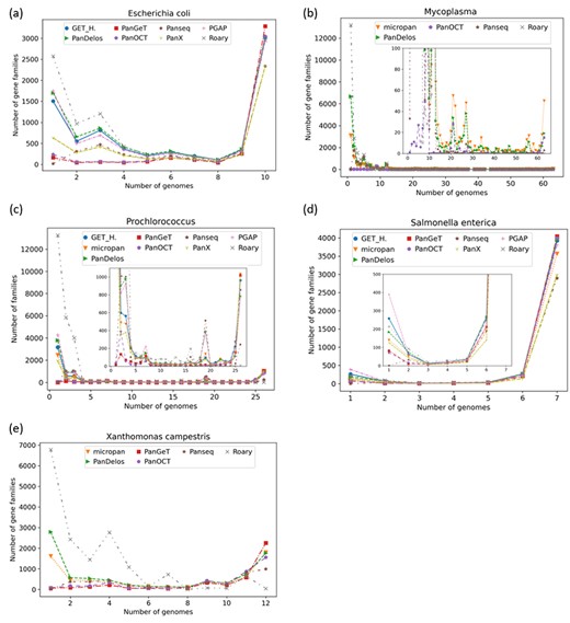
Pangenomic profiles obtained by running the pangenomic tools on collections of genomes belonging to living organisms.
Roary tends to detect a higher number of families when they are involved in a few genomes, while it does not detect core genes. PanSeq does not detect core genes and, in some cases, singletons too. Micropan and PanDelos are on average the tools that extract the highest number of singles, after Roary, but return a large number of core genes. For all collections, the tools generally extract U-shaped profiles, except for the genus Mycoplasma. Tools consistently differ in the number of singletons, families of genes involving few genomes and core families. However, they tend to converge in the right middle part of the profile, with the exception of the core genes.
Discussion and Conclusions
Pangenomic tools are provided as stand-alone software or online platforms. The benefits of the 1st ones are the possibility to embed them into sophisticated frameworks and modify their behaviour changing the source code. An advantage of online platforms is the easier usage and their continuous update. However, they are restrictive in terms of reproducibility and their computational power is often restricted. When using stand-alone tools, reproducibility is assured by the fact that an exact copy of the software used for a given analysis can be retrieved. Homology detection strategies are the core of pangenomic analyses, and they arise critical aspects of computational workflows. Alignment scores are not bijective and sequence similarity is highly dependent on contextual factors. Interpretation of a similarity value between two genes, in relation to a background set of sequences, changes w.r.t. background composition. Good pangenomic methodologies try to solve this problem by applying strategies that include normalized scores, context depended cutoffs, acquisition of additional information such as protein domains and clever usage of BLAST. The use of information not based on sequence similarities, such as protein domains and synteny data, can help accomplish this task.
Alignment of genetic sequences is a useful methodology when comparing closely related genomes for which no singletons or low abundant gene families emerge. Indeed, GET_HOMOLOGUES outperforms other pangenomic tools in this type of benchmark. Different results are obtained using a more realistic scenario as regard synthetic bacterial populations at heterogeneous genomic distances and with an expected presence of low abundant families. In these populations, high performances are achieved by mixing alignment-free measures with clustering (or community detection) techniques. PanDelos and PanX are the tools that show better results in these situations, i.e. on the benchmarks that best resemble real pangenomic contents.
As for performance in terms of execution time, most tools show a strong demand for time requirements. This is due to the use of established approaches, such as BLAST, as a basis for calculating homology between genes. The homology calculation represents the main computational funnel. Time requirement forces that the methodologies limit the number of comparative computations performed at the expense of more sophisticated and precise comparisons. Some, such as EDGAR, use computer clusters to speed-up the computation, but this approach is very expensive. Solutions capable of operating on relatively inexpensive gaming computers may be adopted; they are developed to work with the GPU-GP hardware which is now incorporated in almost all mid-range machines.
Finally, the presented study highlights the need for computational tools for the generation of synthetic populations with realistic pangenomic contents. Such an instrument should combine current knowledge regarding genome evolution in terms of sequence variations acquired during genetic transmissions and acquisition/formation of new genes.
Tools for discovering the pangenomic content in gene-oriented analyses show different performances depending on the properties of the genomes analysed.
Synthetic benchmarks help analyse the performance of tools in relation to the properties of the input genomes.
Methodologies based on alignment-free calculation of gene homology and clustering/community detection techniques have performance advantages over others.
Methods for constructing synthetic benchmarks lack important functionality for studying the extraction of pangenomic content.
Funding
VB and RG are partially supported by GNCS-INDAM and JPND (2019-466-037).
Footnotes
Vincenzo Bonnici is a temporary assistant professor in Computer Science and Bioinformatics at the University of Verona, and senior member of the InfOmics laboratory.
Emiliano Maresi is a PhD student at The Microsoft Research, University of Trento Centre for Computational and Systems Biology.
Rosalba Giugno is an associate professor in Computer Science and Bioinformatics, referent of the Master Degree in Medical Bioinformatics, and PI of the InfOmics laboratory at University of Verona.
References
