


Abstract
The genome-wide discovery of microRNAs (miRNAs) involves identifying sequences having the highest chance of being a novel miRNA precursor (pre-miRNA), within all the possible sequences in a complete genome. The known pre-miRNAs are usually just a few in comparison to the millions of candidates that have to be analyzed. This is of particular interest in non-model species and recently sequenced genomes, where the challenge is to find potential pre-miRNAs only from the sequenced genome. The task is unfeasible without the help of computational methods, such as deep learning. However, it is still very difficult to find an accurate predictor, with a low false positive rate in this genome-wide context. Although there are many available tools, these have not been tested in realistic conditions, with sequences from whole genomes and the high class imbalance inherent to such data.
In this work, we review six recent methods for tackling this problem with machine learning. We compare the models in five genome-wide datasets: Arabidopsis thaliana, Caenorhabditis elegans, Anopheles gambiae, Drosophila melanogaster, Homo sapiens. The models have been designed for the pre-miRNAs prediction task, where there is a class of interest that is significantly underrepresented (the known pre-miRNAs) with respect to a very large number of unlabeled samples. It was found that for the smaller genomes and smaller imbalances, all methods perform in a similar way. However, for larger datasets such as the H. sapiens genome, it was found that deep learning approaches using raw information from the sequences reached the best scores, achieving low numbers of false positives.
The source code to reproduce these results is in: http://sourceforge.net/projects/sourcesinc/files/gwmirna Additionally, the datasets are freely available in: https://sourceforge.net/projects/sourcesinc/files/mirdata
Introduction
MicroRNAS (miRNAs) are critical and key regulators of gene expression [1]. They play important regulatory roles in many fundamental biological processes such as disease development and progression. For example, recent studies demonstrated that miRNAs can serve as tumor suppressors in cancer [2], thus they can assist in diagnosis, prognosis prediction and better therapeutic assessment [3]. However, it is very hard to identify new miRNAs experimentally and this difficulty has led to the development of computational approaches for prediction [4, 5].
The computational prediction of novel miRNAs involves identifying small RNA sequences having the highest chance of being real miRNA precursors (pre-miRNAs). The known pre-miRNAs (deposited in miRBase or MirGeneDB) are usually just a few in comparison to the millions of hairpin-like sequences that have to be analyzed in full genome data. In the past few years, a very large number of strategies have been proposed for tackling this problem. On one side, the advent of high-throughput sequencing technology provided the opportunity of identifying almost all miRNAs that are expressed in a transcriptome. Thus, the discovery of novel miRNAs from RNA sequencing data became very important, giving rise to lots of tools that required this type of data to provide a prediction [6–13]. However, those methods can only detect miRNAs that are expressed in a very specific experimental condition, missing other new candidates because of lack of expression in that particular experiment. On the other side, many different approaches appear that could be used only with the raw genomic sequences. Particularly, methods based in machine learning (ML) have shown to be well suited to this prediction task [14, 15]. In [16] the authors state that existing methods have limited capacity to detect miRNA sequences and precursors with low similarity to the reference set, while ML models can capture more general features that overcome this weakness. This is because most of the ML methods identify candidates in non-coding and non-repetitive regions of the genome by using features that are extracted from typical properties of known pre-miRNAs. These features can be the number of loops, average length or minimum free energy when folding the secondary structure, among many others [17–19]. ML methods learn how to classify according to the values of these features and, moreover, their interactions. This is learnt automatically from the training data and for each species.
Several reviews have analysed the advantages of ML methods for pre-miRNA prediction. For example, the study in [20] reviews 20 tools published before 2018, where 11 out of 20 are ML-based. This was a bibliographic review of papers and tools, which classified and ranked them according to citation number in order to determine development trends in miRNA tools. Differently, our work is not theoretical but rather a practical comparison among several recent ML prediction methods. In [15], 29 pre-miRNA ML-based prediction tools published in the past 10 years are presented and assessed with a number of artificial datasets of varying levels of class imbalance. That is, method performance was analyzed throughout the ratios between the number of known pre-miRNAs and the other sequences, ranging from 1:1 (no imbalance) up to 1:2000 (high imbalance). However, while this review included several algorithms, only small and curated datasets were used, without experiments in realistic genome-wide scenarios. There are no comparisons among ML-based methods with the realistic imbalance existing in genome-wide data. In this context, the class imbalance problem becomes critical and affects the predictors [21]. A very large imbalance ratio (IR) is present between the positive class (a few known pre-miRNAs) and unlabeled data in the rest of the genome, and putatively belonging to the negative class. This quite simple but very important fact may bias the model to the majority class. Therefore, most existing ML proposals for this problem, although reporting very high accuracy, might not be completely reliable in such a scenario. In order to fulfill this lack of comparisons in a realistic scenario, in this study we review and systematically compare the performance of novel pre-miRNA classifiers based on ML, along several publicly available genome-wide datasets of animals and plants, with the real IR of each genome and under the same experimental conditions.
ML classifiers
The first ML methods proposed for miRNA prediction were supervised classifiers. The supervised approach needs both positive (known pre-miRNA) and negative (non-pre-miRNA) sequences in order to build a binary classifier for discriminating between them. The classifier builds a model that must be capable of predicting whether a new point, that is an unlabeled sequence whose class is previously unknown, belongs to one class or the other one. For training the model, the main structural features of known pre-miRNAs are extracted [19]. Support vector machines (SVM) were the first and most widely applied algorithm for this task [22]. In this study, we use a supervised approach of SVM that relies only on the positive-labeled data for building a classification frontier, the one-class SVM (OC-SVM). It was shown that this approach can perform better than standard (two-classes) SVM in pre-miRNA prediction [23, 24].
The first model that has been proposed for pre-miRNA prediction with semi-supervised learning was deepSOM [25]: an architecture with several levels of self-organizing maps (SOMs) [26]. During training, each input data point is assigned to a map unit and weights are adapted in an unsupervised way. When there is no further adaptation of the weight vectors in this SOM, only the data assigned to the neurons having at least one positive class sample (the pre-miRNA neurons) are chosen for training the next map. An important drawback of this model is that a very large number of pre-miRNAs candidates got high scores, thus causing a drop in the precision. The deep ensemble-elasticSOM (deeSOM) [21] introduced two key improvements to the deepSOM. First, each layer can be defined as an ensemble of independent SOMs. All positive samples are fed to every initial SOM while unlabeled samples are randomly split between each one of the members of the ensemble. This allows to reduce the imbalance at SOMs in the ensemble, each one learning a different unlabeled subspace. The second improvement was an algorithm to adaptively adjust the size of each SOM layer depending on the performance of previous layers. This changed the distribution of samples on each layer, allowing a further depuration of pre-miRNA candidates.
The first pre-miRNA predictor for genome-wide based on graphs was miRNAss [27]. This method receives as input a set of labeled feature vectors, which represent sequences and their class: positive for known pre-miRNAs or unlabeled for the rest. An initial graph is built from all the sequences. Then, the nodes topologically far away from the positive examples are labeled as negative examples. Prediction scores are estimated for all the sequences, taking into account that (i) topologically close sequences in the graph must have similar prediction scores; and (ii) the scores have to be similar to the values given for true pre-miRNAs in the label vector. Finally, using the prediction scores assigned to the labeled examples, an optimal threshold is estimated in order to separate the pre-miRNAs candidates from the other sequences.
In the past years, the emergence of deep learning models has led to significant improvements in many fields [28]. These models had been used in several bioinformatics applications, such as the prediction of new miRNAs and their targets [29]. Deep learning is inspired by the representation of biological neural networks and it can be considered today among the best paradigms of ML approaches for supervised classification. A deep neural network can be built from several layers of nonlinear feedforward networks. One of the layer types that are commonly used include latent variables organized layer-wise in deep generative models such as the restricted Boltzmann machines (RBM) [30]. Very recently, in [31, 32] a deep neural network based on RBM (deepBN) for pre-miRNA prediction was proposed, achieving the best performance in comparison to other state-of-the-art methods [15]. Instead of using handcrafted features like the ones in the models described before, there are other deep neural architectures that can learn the features automatically from raw data. The convolutional neural networks (CNN) have been used to classify RNA families (DeepMir) [33] and to identify miRNAs mirtrons [34]. These works use a one-hot-encoding scheme to convert a RNA sequence of |$1 \times N$| nt in an |$4 \times N$| matrix to feed the networks. In other recent work, a long-short term memory neural network (LSTM) was used to learn patterns from the raw sequences and to classify pre-miRNAs (deepMiRGene) [35], where each sequence is coded in a novel way altogether with the predicted folding structure from RNAfold library. Although DeepMir and deepMiRGene reported interesting results in previous works [33, 35], our preliminary tests with genome-wide data showed that training do not converge. Datasets used in the original works were smaller and with very low imbalance. Therefore, in this study the training algorithms were adapted to generate balanced training batches, allowing the classifiers to adjust the error gradient with a similar weight to both classes. These adapted models will be further referred to as balanced-batches DeepMir (bb-DeepMir) and balanced-batches deepMiRGene (bb-deepMirGene).
Materials and experimental setup
Genome-wide data
Full genome datasets from five species were used: Caenorhabditis elegans (CEL), Drosophila melanogaster (DME), Anopheles gambiae (AGA), Homo sapiens (HSA) and Arabidopsis thaliana (ATH). Each dataset requires several weeks of pre-processing in order to extract the hairpins and calculate their features. All sequences and features have been made public to be used as benchmarks for model comparison [36]. We have used these datasets because they include the following: a model organism for animals, CEL; a model organism for plants, ATH; and the genome of HSA given its size and importance. Moreover, included genomes have different numbers of miRNAs, hairpins and imbalances, as can be seen in Table 1. The processing pipeline in [36] was designed to extract and fold all hairpin sequences from the chromosomes and mitochondrial genes. Hairpins are regions of RNA transcripts that fold back on themselves to form short stem-loop structures, which may have bulges and mismatches. This is a very specific characteristic of the pre-miRNAs. The number of bulges and mismatches, even their position in the hairpin, are specific and distinctive characteristics of a pre-miRNA. Unfortunately, non-pre-miRNA sequences can also form hairpins. To extract them, the raw genome of each species was analyzed with a window of 500 nt of length, that is, larger than any known pre-miRNA of the analyzed species. These windows were shifted in small steps to generate overlapped sequences. This cutting strategy ensured that no hairpin was lost. The secondary structure of each sequence was predicted using RNAfold 2.1.8. Any sequence that did not fold properly as a hairpin was discarded. The structures that optimized the folding minimum free energy (MFE) [37] were checked to fulfill a minimum length of 60 nt and 16 base pair matches. For the positive class, BLAST was used to match all the known pre-miRNAs deposited in miRBase v21. All other hairpins are considered as unlabeled class. It can be seen that the number of microRNAs and the total amount of unlabeled hairpins for each of the genomes analyzed are very different for each species. If the number of miRNAs is normalized over the genome size (in pair bases), ATH has a similar ratio to CEL and DME, but it is much higher than HSA and AGA. These relationships hold if the number of miRNAs over the total amount of unlabeled hairpins is calculated for each analyzed genome, which is named imbalance ratio in Table 1.
Genome-wide datasets. Details on the number of labeled and unlabeled sequences. The IR is computed as the ratio between them.
| Dataset | Positive sequences | Unlabeled hairpins | IR |
|---|---|---|---|
| CEL | 249 | 1,737,349 | 1:6977 |
| DME | 307 | 2,066,807 | 1:6732 |
| AGA | 66 | 4,268,407 | 1:64,672 |
| HSA | 1710 | 48,099,855 | 1:28,128 |
| ATH | 304 | 1,355,663 | 1:4459 |
| Dataset | Positive sequences | Unlabeled hairpins | IR |
|---|---|---|---|
| CEL | 249 | 1,737,349 | 1:6977 |
| DME | 307 | 2,066,807 | 1:6732 |
| AGA | 66 | 4,268,407 | 1:64,672 |
| HSA | 1710 | 48,099,855 | 1:28,128 |
| ATH | 304 | 1,355,663 | 1:4459 |
Several features were extracted from these stem loops with miRNAfe [19], such as the ratio of each base in the sequence, the proportion of guanine-cytosine on the sequence, the ratio between guanine and cytosine, the length of the sequence, the number of stem loops and the number of nucleotides in the stem region, among many other. These features were used in OC-SVM, deepBN, deeSOM and miRNAss. Instead, bb-deepMiRGene and bb-DeepMir models do not use hand-engineered features but the raw sequence of each hairpin. The prediction of the secondary structure of each sequence, provided by RNAfold, is used by bb-deepMiRGene as well. Additional details of the feature extraction process can be found in [3] and a detailed description of the features inself is provided in the Supplementary Material, Table S1.
Performance measures
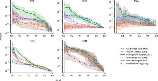
Precision-recall curves for all the methods and datasets. Precision is in log scale. Bold curves are the mean of cross-validation results while the shaded area is the 10–90 percentile range.
Experimental setup
The models with published source code were trained and tested using our genome-wide datasets. Experimental evaluation was designed taking into account the practical considerations of the genome-wide pre-miRNA discovery task. Given that the computational cost of the methods are very high with genome-wide data, hyper-parameter optimization strategies, such as grid-search, can be prohibitive. Thus, the hyper-parameters used for each model are those published by the original authors. These are summarized in the Table S2 of Supplementary Material.
Each ML model was trained independently for each species in Table 1, and evaluated with an 8-fold cross-validation (CV) scheme, for each genome individually, to get an unbiased estimation of performance on unseen data. Each sequence from each genome was labeled either as a positive class (known pre-miRNAs) or unlabeled class. Each fold consisted of independent and non-overlapped training (7/8) and testing (1/8) partitions, each testing partition with the same IR as in the full genome. The pre-miRNA candidate scores obtained by the models for the samples in the test partitions were compared with the known labels to assess model performance. Friedman test and critical difference diagram with post hoc Nemenyi test were used to assess the statistical significance of differences in the |$\hat{AUC}_{PR}$| achieved by each model.
Results
The precision-recall curves for the prediction of novel pre-miRNAs in the genome-wide datasets are shown in Figure 1, for OC-SVM, deepBN, bb-deepMiRGene, miRNAss, deeSOM and bb-DeepMir. These curves were generated using the scores provided by each method. In these figures, the higher the curve the better. As it can be seen, the curves show a low precision when recall is high (bottom right corner of each sub-figure), where most of the candidates are, in fact, false positives. This is considered as a baseline, that is, the model obtains R=1.0 at the cost of classifying all test sequences as positive. As the score threshold is increased (from right to left), low-quality candidates are discarded, rapidly improving precision, but at the cost of losing recall.
In the CEL dataset, it can be seen that bb-DeepMiRGene has an outstanding performance, which can be due to the fact that, differently from the others, this method uses information of both sequence and secondary structure. This indicates that taking into account both information sources seems to be very important for finding good and precise pre-miRNAs candidates. In contrast, in spite that bb-DeepMir is also based on deep learning, it uses only sequence information and has the lowest score. Regarding deepBN, in spite of having reported very good results for pre-miRNA prediction in other scenarios, in this genome-wide dataset the large class imbalance seems to have affected its performance. For high recall, it can be seen that bb-DeepMiRGene reaches the best values, followed by OC-SVM and miRNAss. Regarding high precision, where recall is low, it can be seen that OC-SVM and deepBN lower its performance. These models are not able to deliver a small number of candidates with low FP. Regarding deeSOM, it seems to be the method with a more balanced trade-off between recall and precision.
For the DME dataset, bb-DeepMiRGene and OC-SVM work better again. On this dataset, only bb-deepMiRGene and deeSOM could reach good precision results. In the case of the AGA dataset, it should be noted that there is a very low number of known mirnas, only 57, which seems to deeply affect most of the classifiers. Only bb-deepMiRGene and deeSOM could reach high precision values. The HSA dataset is the largest one and miRNAss needed to build a very large adjacency matrix, which make it not applicable in practice for this amount of sequences. In general, similar behaviours as the dataset before can be observed, except for bb-DeepMir, which reaches here good precision values. Since this data set has a relatively large number of known miRNAs (1,710) and bb-DeepMir uses only sequence information, it seems that there are many similar patterns that are easily found by this method. Here, again, bb-deepMirGene is the best method. Finally, in the ATH dataset, almost all models behave similarly except for bb-DeepMir, which has a very low precision score for moderate recall but reaches a good precision at low recalls.
For a global comparison among all the methods, an assessment of performance was done by measuring the maximum |$F_1$|, maximum MCC score and the |$\hat{AUC}_{PR}$| for each model in each genome (Table 2). In the CEL genome, both |$F1_m$| and |$MCC_m$| measures clearly indicate bb-deepMiRGene as the best method (in bold). In this genome, the following methods with high performance are deeSOM, miRNAss and bb-DeepMir, however, at a long distance from the best one. Regarding |$\hat{AUC}_{PR}$|, bb-deepMiRGene is clearly the best one in this genome. In DME, the best method is deeSOM according to |$F1_m$| and |$MCC_m$|, closely followed by the deep models bb-DeepMir and bb-deepMirGene. According to |$\hat{AUC}_{PR}$|, the last one is by far the best one. In the AGA dataset, bb-deepMiRGene is again the best one, followed by deeSOM and OC-SVM. According to |$\hat{AUC}_{PR}$|, the best one is deeSOM, although very close to bb-deepMiRGene. In the largest genome, HSA, again bb-deepMiRGene, bb-DeepMir and deeSOM are the best ones. Finally, in ATH the best method according to |$F1_m$| is miRNAss and deeSOM is the best according to |$MCC_m$|. In |$\hat{AUC}_{PR}$|, again bb-deepMiRGene is the best one.
Summarized performances for all methods and datasets. |$F1_m$| and |$MCC_m$| are the best F1 and MCC along the precision-recall curve. |$\hat{AUC}_{pr}$| is the logarithmic ratio of the area under the precision-recall curve.
| CEL | DME | AGA | HSA | ATH | |||||||||||
|---|---|---|---|---|---|---|---|---|---|---|---|---|---|---|---|
| |$F1_m$| | |$MCC_m$| | |$\hat{AUC}_{pr}$| | |$F1_m$| | |$MCC_m$| | |$\hat{AUC}_{pr}$| | |$F1_m$| | |$MCC_m$| | |$\hat{AUC}_{pr}$| | |$F1_m$| | |$MCC_m$| | |$\hat{AUC}_{pr}$| | |$F1_m$| | |$MCC_m$| | |$\hat{AUC}_{pr}$| | |
| OC-SVM | 0.012 | 0.047 | 0.342 | 0.002 | 0.015 | 0.292 | 0.013 | 0.033 | 0.240 | 0.004 | 0.014 | 0.197 | 0.153 | 0.121 | 0.625 |
| deepBN | 0.009 | 0.025 | 0.220 | 0.000 | 0.002 | 0.044 | 0.001 | 0.007 | 0.002 | 0.006 | 0.016 | 0.241 | 0.143 | 0.148 | 0.595 |
| deeSOM | 0.037 | 0.063 | 0.378 | 0.075 | 0.120 | 0.166 | 0.019 | 0.023 | 0.367 | 0.028 | 0.035 | 0.365 | 0.172 | 0.187 | 0.649 |
| miRNAss | 0.030 | 0.044 | 0.357 | 0.001 | 0.005 | 0.020 | 0.008 | 0.007 | 0.071 | - | - | - | 0.212 | 0.173 | 0.676 |
| bb-DeepMir | 0.028 | 0.023 | 0.190 | 0.053 | 0.015 | 0.048 | 0.009 | 0.009 | 0.109 | 0.038 | 0.050 | 0.457 | 0.085 | 0.060 | 0.475 |
| bb-deepMiRGene | 0.103 | 0.095 | 0.567 | 0.060 | 0.040 | 0.387 | 0.058 | 0.045 | 0.336 | 0.072 | 0.031 | 0.511 | 0.195 | 0.179 | 0.686 |
As it can be seen in Table 2, the performance of the methods is very variable according to the size and imbalance of the genome data evaluated. Therefore, by using one measure alone, it is very difficult to indicate only one best method for all cases. However, since precision is in takes different orders of magnitude and the |$\hat{AUC}_{PR}$| is logarithmic scale, this measure gives more weight to the methods that reach better precision scores. High precision is very desirable when searching for new pre-miRNAs candidates in order to have less false positives to test. According to |$\hat{AUC}_{PR}$|, it can be seen that bb-deepMiRGene reaches the higher values in most datasets, with exception of AGA, in which deeSOM is the best one. The very large class imbalance effect can be seen specially in AGA, where deepBN, miRNAss and bb-DeepMir cannot reach good results, while on ATH, the scores are high for all models. In order to provide a statistical analysis of results, a Friedman test was done, showing that differences in the |$\hat{AUC}_{PR}$| results are statistically significant (p = 3,3e-15). Critical difference (CD) diagram (Fig. 2) shows that bb-deepMiRGene and deeSOM are the best methods for the genome-wide prediction of pre-miRNAs. OC-SVM can reach a good |$\hat{AUC}_{PR}$|, especially for high recall, but it cannot reach high precision values. These comparative results have shown that while the genome-wide imbalance affected all the methods, deep models (deeSOM and deepMiRGene) were the most robust for all species.
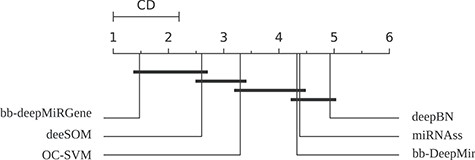
CD diagram for the pre-miRNA prediction methods along all genome-wide datasets.
Another relevant aspect of the methods reviewed, besides performance, is the computational cost. Using the same hardware specifications and the CEL dataset, OC-SVM took, on average, 7s for training each fold. This was the fastest method since it uses only the known positives for training and does not model the negative class. OC-SVM was followed by bb-DeepMir with 10 min and deeSOM with 20 min on average for each fold. However, miRNAss took 23 hs to train one fold because the adjacency matrix must be calculated pairwise among every sequence. Similarly, bb-deepMiRGene took 37.5 hs because of the conversion from sequences to embedding for such large genome data. The cost of predicting new sequences was negligible in all the cases after the models were trained.
Another important issue, from a very practical point of view: how many wet experiments should be done in order to find high-quality and true novel pre-miRNAs in the large quantity of sequences of a full genome? In order to answer this question a detailed analysis of the pre-miRNA candidates provided by the models evaluated is presented in Figure 3. Each sub-figure shows the number of sequences considered as candidates (C = TP + FP) at each score threshold along with the number of TP from the testing partition. At the upper right corner is the initial number of sequences from the test partition presented to each model, including the well-known pre-miRNAs labeled as positives. For example, in the case of the CEL dataset there are 32 TP for 217,138 candidates. At the left of each sub-figure is shown how many testing true positives have remained with the highest score threshold, these are the top pre-miRNAs candidates of each method. As the threshold is increased, from right to left in the figure, the slope in the curves shows that large quantities of low-quality candidates are discarded but TP are reduced very slowly, until only a few TP remains with different numbers of candidates. In summary, for these figures the lower the curve the better is the method.
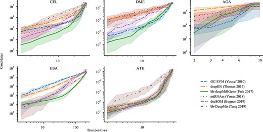
Candidates-TP curves for the five datasets. Bold lines are the mean values for test partitions, and the shaded area is its 10–90 percentile range.
In the CEL dataset, bb-DeepMiRGene could reach the lowest number of candidates for each TP value. For example, if 10 TPs are preserved, the output candidates will be on average 506 for bb-deepMiRGene, 2023 for OC-SVM, 2133 for deeSOM, 2515 for miRNAss, 7337 for deepBN and 17,937 for bb-DeepMir. Similarly, in order to have 2 TPs, the candidates numbers provided by each method will be 34 for bb-deepMiRGene, 520 for OC-SVM, 123 for deeSOM, 310 for miRNAss, 1110 for deepBN and 850 for bb-DeepMir. This means that bb-deepMiRGene provides between 3 and 25 times less candidates than the other methods to discover the same number of TP. As a direct consequence, less wet experiments would be needed to confirm the novel pre-miRNAs. In DME and AGA, it is clear how miRNAss, deepBN and bb-DeepMir produce at least one order of magnitude more FP than the other methods for low TP. In HSA, it seems that there are two groups. First, it can be seen that OC-SVM and deepBN cannot reduce the number of candidates further than 1000. Instead, bb-DeepMir, bb-deepMiRGene and deeSOM reach a very low candidate number, in the order of 100 sequences for 2 TP. In this case, bb-DeepMir seems to reach even lower values but variance is very high. For ATH, all methods but bb-DeepMir have similar behaviour. It is interesting to note that for bb-deepMiRGene and deeSOM, the best 10 candidates would include, on average, 2 TP, which is an outstanding result from a practical point of view.
Finally, all these comparative results illustrate a very important aspect that should be measured in all methods developed and used for pre-miRNA prediction. Drastically reducing the candidates is an important factor to reduce the costs of wet experimental confirmation. The most common case in a real genome-wide application would have millions of hairpins-like sequences, while it is commonly expected that only a few hundreds of them might contain true miRNAs. Thus, in a pre-miRNA classifier the ability for predicting a reasonable number of candidates to be tested in wet experiments is a characteristic of paramount importance. In this regard, the adapted version of bb-deepMiRGene, with balanced batches in the training, and the deeSOM (originally designed for high imbalance) are the best methods for genome-wide pre-miRNA prediction.
Conclusion
In this work we have compared several recent computational models for pre-miRNA discovery. For the first time, the extensive use of genome-wide data from five genomes (C. elegans, D. melanogaster, A. gambiae, H. sapiens and A. thaliana) allowed to compare the models in the same experimental conditions, testing them in a realistic scenario. Experimental results demonstrated that bb-deepMiRGene, a deep-learning network using the sequential and structural information of sequences, outperforms other state-of-the-art methods. This indicates the importance of taking into account both information to train deep learning models for finding pre-miRNAs candidates in genome-wide data. Additionally, deeSOM, a semi-supervised method that uses structural features as input, also reaches good performance, especially taking into account the precision for a low number of candidates.
Six novel pre-miRNA prediction models based on machine learning were tested on five genome-wide datasets.
The models based on deep learning showed the best performances in all datasets.
The deep model that used information of both sequence and secondary structure has obtained the best results for genome-wide data.
Further research on deep learning based methods, with more realistic genome-wide datasets, is needed to improve current pre-miRNAs prediction.
Acknowledgments
We acknowledge the support of NVIDIA Corporation with the donation of the Titan Xp GPU used for this research.
Funding
This work was supported by Agencia Nacional de Promocion Cientifica y Tecnologica (ANPCyT) PICT 2018 3384.
L. A. Bugnon holds a postdoctoral position at sinc(i) since 2017. His research interests include automatic learning, pattern recognition and signal and image processing, with applications to bioinformatics, biomedical signals and affective computing.
C. Yones has a postdoctoral position at sinc(i) since 2017. His research interests include machine learning, data-mining and semi-supervised learning, with applications in bioinformatics.
D.H. Milone is a full professor in the Department of Informatics at Universidad Nacional del Litoral (UNL) and a principal research scientist at CONICET. He is the director of sinc(i). His research interests include statistical learning, signal processing and neural and evolutionary computing, with applications to biomedical signals and bioinformatics.
G. Stegmayer is an assistant professor in the CONICET, Argentina. Her current research interests involve machine learning, data mining and pattern recognition in bioinformatics.
sinc(i) - Research Institute for Signals, Systems and Computational Intelligence. Research at sinc(i) aims to develop new algorithms for machine learning, data mining, signal processing and complex systems, providing innovative technologies for advancing healthcare, bioinformatics, precision agriculture, autonomous systems and human–computer interfaces. The sinc(i) was created and is supported by the two major institutions of highest education and research in Argentina: the National University of Litoral (UNL) and the National Scientific and Technical Research Council (CONICET).
References
