


Abstract
Next-generation sequencing (NGS) technology has revolutionised human cancer research, particularly via detection of genomic variants with its ultra-high-throughput sequencing and increasing affordability. However, the inundation of rich cancer genomics data has resulted in significant challenges in its exploration and translation into biological insights. One of the difficulties in cancer genome sequencing is software selection. Currently, multiple tools are widely used to process NGS data in four stages: raw sequence data pre-processing and quality control (QC), sequence alignment, variant calling and annotation and visualisation. However, the differences between these NGS tools, including their installation, merits, drawbacks and application, have not been fully appreciated. Therefore, a systematic review of the functionality and performance of NGS tools is required to provide cancer researchers with guidance on software and strategy selection. Another challenge is the multidimensional QC of sequencing data because QC can not only report varied sequence data characteristics but also reveal deviations in diverse features and is essential for a meaningful and successful study. However, monitoring of QC metrics in specific steps including alignment and variant calling is neglected in certain pipelines such as the ‘Best Practices Workflows’ in GATK. In this review, we investigated the most widely used software for the fundamental analysis and QC of cancer genome sequencing data and provided instructions for selecting the most appropriate software and pipelines to ensure precise and efficient conclusions. We further discussed the prospects and new research directions for cancer genomics.
Introduction
Next-generation sequencing (NGS) technology has produced a wealth of cancer genomics data, leading to the need for efficient and accurate software and workflow/pipelines for its processing and interpretation. For example, Atlas2 is an integrative workflow specialised for variant calling involving data of three exome capture sequencing methods (SOLiD, Illumina and Roche 454) [1]. GATK4 is a robust variant analysis pipeline and toolkit available for many types of sequencing platforms [2]. The unified analytic framework presented by DePristo allows the discovery and genotyping of variants among multiple samples, simultaneously across five sequencing technologies and three experimental designs [3]. Meanwhile, GenomeVIP is a framework for performing variant discovery and annotation from whole-genome sequencing (WGS) and whole-exome sequencing (WES) data [4]. Furthermore, cloud-based workflow system such as Butler, Rainbow and MC-GenomeKey provide solutions for facilitating population-scale human genomic studies [5–7]. However, detailed analyses of these workflow systems are not available to users, and they either focus solely on the variant discovery or lack the necessary quality control (QC) measures.
Cancer genome analysis comprises raw data pre-processing and QC, sequence alignment and variant calling, followed by variant annotation and visualisation. Although some of these software and pipelines are prevalent and widely used in a few large-scale studies, three issues remain: (i) there is a lack of professional guidance for selecting between suitable software with similar functions; (ii) certain well-known processes are not suitable for particular applications; and (iii) multi-dimensional QC is ignored.
In this review, we discussed how to select suitable software and workflow strategy as well as to conduct quality management according to the four steps detailed in Figure 1: (i) raw sequence data pre-processing and QC, (ii) sequence alignment and QC, (iii) variant detection and filtering and (iv) variant annotation and visualisation. Most research on cancer genome sequencing focuses on only one aspect of the analysis or lacks a detailed description of the quality control. This review will fill in the gaps by providing comprehensive and detailed recommendations for cancer genome sequencing analysis.
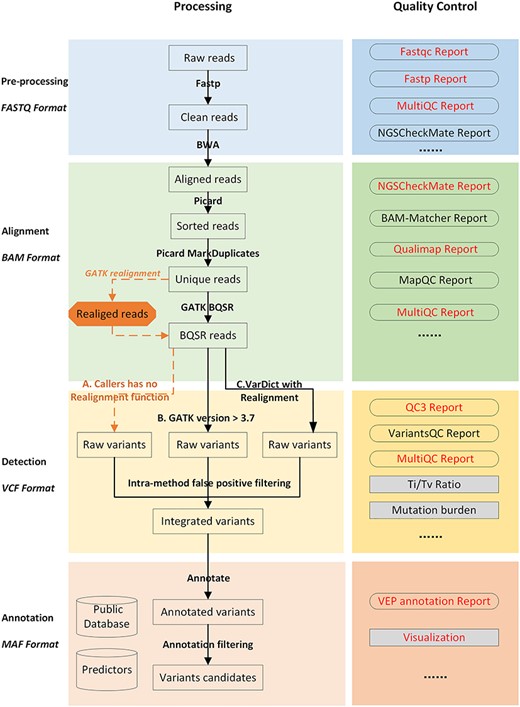
Detailed overview of the NGS data analysis pipeline with quality control. Analysis of cancer genome sequencing data of WGS/WES/Target consists of four steps: (i) raw data processing (shown in blue); (ii) alignment data processing (shown in green); (iii) short variants (SNVs/indels) calling and false-positive filtering (shown in yellow); and (iv) variant annotation and visualisation (shown in orange). Quality control (QC) for each step is listed on the right in a darker colour. Red font is used to emphasise the importance of QC reports. There are two alternative routes after unique reads have been generated. The steps denoted by orange dashed lines indicate that realignment is required when the variant caller has no realignment function. Realignment should not be conducted when choosing a variant caller with realignment function, such as VarDict or GATK version 3.7 or higher. Sample matching checks (orange arrows) can be conducted using NGSCheckMate in ‘Raw data processing’, with BAM-Matcher or NGSCheckMate in ‘Aligned data processing’, and with NGSCheckMate until ‘Variant data processing’. However, this step is only required once, and we recommend that it is conducted during ‘Aligned data processing’.
Raw sequence data pre-processing and QC
The QC and pre-processing of raw sequence data in the FASTQ format are necessary to obtain high-confidence results. QC generates text or graphic reports that identify issues deriving from either the sequencer or the library material, whereas pre-processing trims sequence artefacts (typically platform-specific PCR primers and adapters) and filters out substandard reads to generate clean sequences for subsequent analysis.
Several tools are publicly available for the manipulation of FASTQ files. We have summarised the functions and features of 15 of these open-source tools and have listed the number of citations (as of 9 January 2020; normalised by years since publication) to indicate their popularity in Table 1. Also, we classified these sophisticated tools into three main categories, namely, QC tools, pre-processing tools and all-in-one tools, based on the differences in their methods and design functionalities that facilitate their use by those who lack relevant analytical experience. To further distinguish these tools, we systematically explore and compare the results obtained from three WES cases, therefore allowing us to make recommendations on tool selection and prioritisation according to particular needs.
Raw data analysis tools
| Tool feature | Function | (i) Quality control tools | (ii) Pre-process tools | (iii) All-in-one tools | ||||||||||||
|---|---|---|---|---|---|---|---|---|---|---|---|---|---|---|---|---|
| Software | FastQC | MultiQC | NGS-Bits (ReadQC) | FASTX-Toolkit | Cutadapt | TrimGalore | Trimmomatic | Skewer | PEAT | SOAPnuke | PRINSEQ | NGS QC Toolkit | FaQCs | AfterQC | Fastp | |
| Publication feature | Citations/year | 384.20 | 124.25 | 0.67 | 22.30 | 737.56 | 37.13 | 2148.50 | 64.50 | 4.20 | 26.67 | 270.00 | 178.13 | 11.83 | 16.00 | 86.00 |
| Installation | Installation | B/F | B/C/P | B/C/F | B/F/C | B/P | B/F | B/F | B/C/F | C/F | C | B/F | C | B/C | B/C/F | B/C/F |
| Performance | Time (hh:mm:ss) | 00:03:11 | 00:00:06 | 00:09:17 | NA | 00:10:29 | 00:05:56 | 01:03:22 | 00:22:55 | 00:59:35 | 00:07:08 | 08:23:20 | 01:04:09 | 01:09:17 | 04:02:50 | 00:07:03 |
| Report feature | Format | html; text | html; text; json | qcML, tsv | text | stdout | text | text | stdout | text | text | html | html; text | pdf; text | html; json | html; pdf; json |
| Visualisation | Before | Post | Post | Post | χ | χ | χ | χ | χ | χ | Post | Post | Post | Both | Both | |
| Interactive | χ | ✓ | χ | χ | χ | χ | χ | χ | χ | χ | χ | χ | χ | ✓ | ✓ | |
| Development feature | Multi-threading | ✓ | χ | χ | χ | ✓ | ✓ | ✓ | ✓ | ✓ | ✓ | χ | ✓ | ✓ | ✓* | ✓ |
| Multi-sample | ✓ | ✓ | χ | χ | χ | χ | χ | χ | χ | χ | χ | χ | ✓ | ✓ | χ | |
| Quality profile | Duplicated reads | ✓ | χ | χ | χ | χ | χ | χ | χ | χ | ✓ | ✓ | χ | ✓ | χ | ✓ |
| Overlapping analysis | χ | χ | χ | χ | χ | χ | χ | χ | χ | χ | χ | χ | χ | ✓ | ✓ | |
| Sequencing error profiling | χ | χ | χ | χ | χ | χ | χ | χ | χ | χ | χ | χ | χ | ✓ | ✓ | |
| Processing function | PE or SE | SE | χ | ✓ | SE | ✓ | ✓ | ✓ | ✓ | ✓ | ✓ | ✓ | ✓ | ✓ | ✓ | ✓ |
| Detect adapter automatically | χ | χ | χ | χ | χ | χ | χ | χ | ✓ | χ | χ | ✓ | χ | ✓ | ✓ | |
| Cut adapter | χ | χ | χ | ✓ | ✓ | ✓ | ✓ | ✓ | ✓ | ✓ | ✓ | ✓ | ✓ | ✓ | ✓ | |
| Convert quality | χ | χ | χ | χ | ✓ | ✓ | ✓ | ✓ | ✓ | ✓ | ✓ | ✓ | ✓ | χ | ✓ | |
| Quality filtering | χ | χ | χ | ✓ | χ | ✓ | ✓ | ✓ | ✓ | ✓ | ✓ | ✓ | ✓ | ✓ | ✓ | |
| Trimming 3′ or 5’ | χ | χ | χ | ✓ | ✓ | ✓ | ✓ | ✓ | ✓ | ✓ | ✓ | ✓ | ✓ | ✓ | ✓ | |
| Sequence complexity | χ | χ | χ | χ | χ | χ | χ | χ | χ | χ | ✓ | χ | ✓ | χ | ✓ | |
| UMI | χ | χ | χ | χ | χ | χ | χ | χ | χ | χ | χ | χ | χ | χ | ✓ | |
| Compressed file | ✓ | ✓ | ✓= | ✓≈ | ✓ | ✓ | ✓ | ✓ | ✓ | ✓ | χ | ✓ | ✓= | ✓ | ✓ | |
✓, software has this function; χ, software does not have this function; *, software has this function, but no parameters were provided; #, SE; =, only input; ≈, only output.
B, install with BioConda or running Docker containers built by BioContainers; C, install by compiling from source; D, Docker container independent of BioContainer; F, free from compile by providing a pre-compiled binary file or script of Perl; P, install with pip.
‘Interactive’ row indicates reports that include interactive figures that can respond to user events like mouse hover.
‘Time’ was the average running time of processing 3 WES samples of Illumina paired-end sequencing.
QC tools
Dedicated QC tools such as FastQC and ReadQC (a module in NGS-Bits) are excellent for highlighting potential problems in sequence data [8, 9]. FastQC illustrates QC metrics exhaustively and efficiently by producing graphs and tables in an HTML-based permanent report which includes read and base counts, read length, base composition distribution, GC content distribution and quality score curve statistics. In addition, FastQC checks the quality score encoding scheme and provides warnings and error thresholds that can be defined by the user. Conversely, the ReadQC report is relatively simple, consisting of read and base counts, read length, Q20, Q30 and two plots in qcML format. FastQC was faster than ReadQC in the testing using WES data, owing to the down-sampling strategy in FastQC.
Identifying sequencing quality issues by checking the reports of each sample in a cohort study can be inconvenient. MultiQC solves this problem by creating an individual report that can flexibly integrate quality reports from various QC tools and sample sets, allowing overall trends and deviations in large-scale sample studies to be identified rapidly and efficiently [10]. Therefore, we recommend utilising MultiQC in cohort studies to obtain insights into the quality of all samples and avoid batch effects.
Pre-processing tools
Pre-processing tools manipulate FASTQ files by trimming adapters, filtering low-quality sequences, correcting base errors, etc., to prepare the files for alignment. The most significant of these features are adapter detection and trimming because adapter sequences will be read when the DNA fragment is shorter than the specified sequencing length, resulting in reads with unfavourable adapter sequences, known as adapter contamination. FASTX-Toolkit, Cutadapt, TrimGalore, Trimmomatic, Skewer and SOAPnuke are all common examples of pre-processing software designed to recognise and remove adapters based on sequence-matching algorithms that require a series of adapter sequences [11–15]. Conversely, paired-end adapter trimmer (PEAT) detects adapter sequences with indefinite length and a higher detection accuracy by using an overlap analysis algorithm that exploits overlapping fragments of paired forward and reverse reads [16]. Compared with sequence matching-based algorithms, overlap analysis-based algorithms have the distinct advantage of being able to detect and remove shorter adapters. Because the overlap analysis-based method does not require prior adapter sequences, it is particularly useful for analysing large-scale cancer genomics data from multiple different technical platforms that may use different adapters.
Low-quality sequences should also be discarded from FASTQ files to ensure reliable interpretation; therefore, careful attention should be paid to the quality of the encoding scheme. For instance, Phred33 is encoded with an ASCII character add by 33 (ASCII 0–62) and is used by the Sanger/Illumina 1.9+ sequencer, whereas Phred64 is encoded by 64 (ASCII 59–126) and is used before the Illumina pipeline CASAVA 1.3 [17]. FastQC automatically detects and reports a sequencer version, which can be used to infer ASCII quality encoding [8]. Most raw sequence data pre-processing tools support both quality encoding schemes and can convert from Phred64 to Phred33, except for the FASTX-Toolkit, which can only process Phred64 FASTQ files. In addition, Trimmomatic can convert from Phred33 to Phred64 and can automatically check the quality format if the encoding scheme has not been specified by the user. To provide further insight, we tested these tools with three WES samples of Illumina paired-end sequencing and identified numerous additional beneficial features, including installation, report format and support for paired-end reads of these pre-processing tools (Table 1). This summarised table would help practitioners compare the tools more easily and select one that is most suitable for certain applications; for instance, SOAPnuke can be scaled to multiple working nodes for parallel computing using a Hadoop MapReduce framework to cope with a vast volume of sequencing data [14]. Further, if researchers intend to view the quality trend of multiple samples in a large-scale study, they can quickly locate the software ‘MultiQC’ through the ‘Multi-sample’ line in ‘Development feature’; if data originates from different sequencers or the adapters of sequencing batches are unknown, one can readily find ‘PEAT’, ‘NGS QC Toolkit’, ‘AfterQC’ and ‘Fastp’ to automatically detect adapters through the line of ‘Detect adapter automatically’ in ‘Processing functions’.
All-in-one tools
Neither QC tools nor pre-processing tools alone can address and process all the issues in raw sequence data simultaneously; therefore, the conventional approach is to use FastQC for QC, Cutadapt to remove adapters and Trimmomatic to filter reads as a QC-‘Pre-process-QC (optional)’ workflow. TrimGalore integrates both pre-processing and QC functions by internally using Cutadapt to perform adapter trimming and quality filtering and then FastQC on the resulting files to provide a quality report [15]. However, TrimGalore runs faster than Cutadapt in paired-end sequencing by processing each read individually in single-end mode and then performing a ‘validation’ run for both trimmed files. Such all-in-one tools have significantly improved raw data analysis by performing QC, adapter trimming, quality filtering and many other processes in a single FASTQ file scan, which serves to significantly simplify the work associated with raw data processing.
PRINSEQ is the first all-in-one processing tool available as a command-line program or web interface [18]. However, its lack of support for multithreading and compression formats means that it is very time-consuming when completing statistical reports for large datasets, thus dramatically limiting its use in cancer genomics research. While the NGS QC Toolkit supports both Illumina and Roche 454 platforms and generates an HTML-based report after processing, it runs slowly because its parallel mode uses one thread for each separate input file [19]. Fastp and AfterQC both produce interactive reports before and after pre-processing, thereby enabling users to hover over points or zoom in on figures to permit direct scrutiny. Moreover, both automatically detect and remove adapters using an overlap analysis algorithm [20, 21]. Additionally, both Fastp and AfterQC evaluate sequencing errors in paired-end data and correct possible wrong bases, which is essential for low-frequency variant calling. Unfortunately, AfterQC runs relatively slowly; hence, it is overly time-consuming when processing large FASTQ files, such as high-depth sequence data [20]. Conversely, Fastp has comprehensive functions and can carry out effective manipulations simultaneously and is thus is suitable for automated raw data processing in the routine analysis of cancer genomics data.
In summary, although QC-only tools are highly efficient for reporting quality metrics, all-in-one tools outperform separate QC, pre-processing tools or tools based on a combination of the two via integrating functionalities to address more problems without sacrificing efficiency effectively. As shown in Figure 1, we, therefore, recommend FastQC for producing single sample quality reports, MutltiQC for producing the overall statistics of a set of samples and all-in-one tools for the QC and pre-processing of raw sequence data due to their efficient operation and functionalities.
Sequence alignment and QC
A fundamental part of cancer genome sequencing is the alignment or mapping of short DNA reads to a human reference genome. The main difficulty of this process is mapping each short read to a large reference genome while distinguishing between true variants and sequencing errors. To overcome this challenge and handle growing quantities of short DNA sequence reads, many alignment tools have been proposed since 2008. Fonseca et al. maintained an up-to-date compendium of over 80 aligners, of which at least 40 can be used to align short DNA sequences [22].
Cancer genome sequencing is primarily launched with scope for paired-end short reads. It is essential to consider the input data characteristics that a mapper is designed for when selecting mappers. For instance, mappers (such as Bowtie2 and BWA MEM) that exploit sequencing quality scores can reduce alignment errors by assigning weaker penalties for mismatches in locations with low-quality scores; and the support for paired-end reads helps to detect alignment errors as well as improve sensitivity and specificity [22].
The different output characteristics of each mapper should also be taken into consideration because mapping quality scores and their thresholds vary between mappers. BWA-MEM assigns each read with a mapping quality score between 0 and 70 to reflect the accuracy of its mapping; a higher score represents more accurate mapping results [23]. However, Bowtie and Bowtie2 use a mapping quality range of 1–255, which relates to ‘mapping uniqueness’; a higher mapping quality is assigned to more unique alignments [24, 25].
After the original alignment of short reads, several recalibration steps are carried out, including the sorting of reads by alignment position, the marking or removal of duplicated reads, the remapping of reads around short insertions and deletions (indels) and the recalibration of read quality. These steps are designed to make the alignment more accurate and prepare for the variant calling step; however, if misused, more false positives will be introduced.
A notable example of a recalibration step is local realignment. Indels are common and functionally essential types of sequence polymorphism. Unlike single-nucleotide polymorphisms (SNPs), indels make sequence mapping more complicated, resulting in alignment artefacts that may lead to a high false-positive rate when detecting single-nucleotide variations (SNVs) around indels. Performing local realignment before variant detection significantly improves read alignments, reduces the false-positive rate, provides enhanced performance for detection of indels and results in higher accuracy in the calculation of variant allele frequency (VAF) [26, 27]. DePristo et al.’s research address the benchmarked effects of indel realignment as well as mathematics behind the algorithms [3].
To reduce the false-positive rate in SNV detection and to improve the accuracy of indel detection, the local realignment on indel regions, using tools such as GATK, SRMA and ABRA (Figure 1A), is commonly performed [26–28]. An alternative strategy is the new variant caller VarDict, which internally triggers local realignment in indel regions and simultaneously identifies mismatches as evidence of indels, thereby improving the accuracy of indel detection [29]. In addition, the command ‘mpileup’ in SAMtools utilises a per-base alignment quality score (parameter ‘B’), which is the Phred-scaled probability of a read base being misaligned, to help reduce the number of false SNVs caused by mismatches around indels [30].
It is essential to bear in mind that the performing local realignment repeatedly may cause over-correction. In a work by Guo et al., the consecutive application of BAQ and GATK’s local realignment functions did not reduce the number of false-positive SNPs but, instead, introduced additional false positives [31]. The GATK team have eliminated realignment in the Mutect2 and HaplotypeCaller pipeline for GATK 3.7 and higher and have adopted a strategy of read reassembly in active regions covering indels in their new pipeline (Figure 1B). Similarly, we do not recommend using callers with a realignment function for input files that have been processed using a separate local realignment tool (Figure 1C).
Cancer genome sequencing mainly involves WGS, WES and gene-panel sequencing for specific genes associated with cancer risk. Thus, it is important to determine the different QC parameters for these types of sequencing data.
The main QC parameter for WGS data is average depth (also known as the sequencing coverage), which is required for the accurate and reliable calling of variants and the estimation of VAF. However, average depth is easily skewed by a short region with a significantly higher depth, which can be quickly identified from depth distribution with an extended tail if regions of extremely high depth exist. Thus, it is more meaningful to exclude extremely high-depth regions when calculating average depth.
Because most of the known pathogenic mutations are found in the coding regions, it is more practical to limit data sequencing and analysis to regions of exons or a set of genes relevant to particular cancer [32]. Thus, WES and gene-panel sequencing are being incorporated into clinical practice because they are easier to manage in terms of cost and complexity of subsequent analysis. For capture-based target sequencing technology, it is important to consider capture efficiency. Clark et al. compared three hybridisation techniques for WES, namely, Nextera and TruSeq from Illumina Inc, SureSelect from Agilent Technologies and SeqCap EZ from Roche NimbleGen and found at least 90% capture efficiency in all three [33]. The calculation of capture efficiency is more meaningful when ignoring bases with low sequencing/mapping quality or low depth, as these bases do not provide sufficient evidence for variant calling. Hence, Bamdst and Picard module named CollectHsMetrics estimates the efficiency using a strategy of filtering low-quality reads [34]. Low capture efficiency can indicate low complexity of library, suboptimal probe hybridisation conditions or low stringent washes.
Sample matching is checked at the alignment stage to ensure that data from the same subject are correctly labelled. NGSCheckMate supports input files in FASTQ, BAM and variant call format (VCF) for sample matching verification. However, it is time-consuming for files in FASTQ format as the software needs to search for a k-mer sequence spanning specific SNPs to obtain read counts and calculate VAFs [35]. BAM-matcher is an alternative tool that provides a rapid pairwise comparison of BAM files by comparing the genotypes at pre-determined genomic locations [36]; however, the software does not support sample consistency examination for cohort studies, unlike NGSCheckMate. Alternatively, Somalier is designed to rapidly measure sample relatedness with BAM files by extracting informative genetic variation to a binary format called ‘sketch’ across 17 384 sites. It also supports reads aligned to genome build GRCh37 and GRCh38. However, understanding the HTML report of Somalier requires bioinformatics expertise [37]. Additional tools supporting the sample matching check include Peddy, seqCAT and HYSYS; however, they only check the matching with VCF files [38–40].
Several tools are used to perform QC and manipulate alignment data. For instance, SAMtools provides universal tools for processing mapping data, such as sorting (sort), indexing (index), depth statistics (depth) and alignment viewing (view) [23], whereas Qualimap is a platform-independent application that examines alignment data and provides a holistic view of the alignments to help identify mapping bias [41]. Additionally, MapQC in NGS-Bits inspects mapping information and provides results in the figures and tables [9]. Picard outperforms SAMtools when sorting, marking or removing duplicates from aligned sequences and can be used as an integrated part of GATK in addition to being a stand-alone application.
In summary, the alignment process is an important step in cancer genome sequencing. Although many programs map short DNA sequencing reads to a reference genome, we recommend BWA (BWA MEM) as it works well in conjunction with downstream analysis tools. For example, GATK integrates BWA into their pipelines and calls variants based on mapping scores of BWA. Moreover, BWA has been adopted in many large studies, such as TCGA and Pan-Cancer Analysis of Whole Genomes (PCAWG); we then recommend Picard to sort and remove duplicate reads. Considering the local realignment function of callers in the variation identification step, researchers should be aware whether and how to conduct local realignment and then complete base quality recalibration using GATK. Qualimap could also be used to provide detailed alignment quality statistics, while sample consistency should be checked with NGSCheckMate in tumour-normal pairwise cohort studies or with Somalier in cancer or germline studies, which is essential in cancer genomics research. All of these recommendations concerning the alignment stage are provided in Figure 1.
Variant detection and filtering
The most common application of cancer genome sequencing in clinical settings is the detection of short and structural variants with respect to a human reference genome, which has greatly stimulated the development of variant detection software [29, 42–50]. To improve the accuracy of detection, many callers also provide a corresponding filtering strategy; however, callers usually differ in their detection algorithms, filtering methods and thus output, particularly when handling sequence data with various characteristics (e.g. sequencing platform, capture regions, depth).
To date, a considerable number of studies have been published comparing the sensitivity, accuracy and performance of different variant detection software for WGS data, WES data and gene-panel sequencing data. For instance, Sandmann et al. evaluated eight tools (VarScan, GATK HaplotypeCaller, Platypus, LoFreq, SAMtools, FreeBayes, SNVer and VarDict) using both real and simulated non-matched datasets [51], whereas Krøigård et al. focused on five real tumour-normal paired samples and nine callers (EBCall, MuTect2, Seurat, Shimmer, Indelocator, Somatic Sniper, Strelka, VarScan2 and Virmid) [52]. The sensitivity of callers to sequencing depth has been investigated for both WES and targeted deep sequencing data; Xu et al. compared the performance of five callers (GATK UnifiedGenotyper, MuTect2, Strelka, SomaticSniper and VarScan2) on SNV detection using amplicon and WES data [53]. However, the versions of the tools evaluated in these studies may not be the most recent, and some callers only detect one variant signal (SNVs or indels). Further, there is a lack of ground truth for some real datasets.
Here, we limited our comparison to four continuously updated and commonly used tools, namely, VarDict (version 1.5.7 in Java), Mutect2 (GATK 4.1.1), VarScan2 (version 2.4.3) and Strelka2 (version 2.9.10) because these are always kept up-to-date and can detect both SNVs and indels in one run. We used four tumour-normal samples with ground truth and standard baseline filtering (VAF > 0.01, depth of both tumour and normal data were at least 500×) provided by the National Center for Clinical Laboratories in China (NCCL). The samples were sequenced using an Illumina Hiseq 2500 platform with a target region of 1.76 million bases and an average sequencing depth of 2700×. The test results are shown in Figure 2 (A, tumour-normal matched samples; B, tumour-only samples; C, agreement of callers) and indicate that VarDict performs the best in terms of precision and recall rate for tumour-normal matched samples.
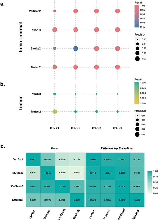
Performace of variant calling tools. (A) Performance of tools (VarDict, Mutect2, VarScan2 and Strelka2) on short somatic variant calling with tumour-normal samples (gene-panel sequencing samples B1701-B17NC, B1702-B17NC, B1703-B17NC, B1704-B17NC). (B) Performance of tools (VarDict and Mutect2) on short somatic variant calling tools with tumour-only samples (gene-panel sequencing samples B1701, B1702, B1703, B1704). The size of the circle correlates with precision: larger size corresponds to the higher precision of the tool. The colour of the circle represents the recall rate: darker colour (pink in tumour-normal samples; blue in tumour-only samples) means a higher recall rate. (C) Pairwise comparisons between VarDict, Mutect2, VarScan2 and Strelka2 for the gene-panel sequencing of B1701. The matrix depicts agreement between the variant callers. The numbers in the first four columns were calculated from variants without baseline filtering (Raw), while the numbers in the last four columns were calculated from baseline filtered variants (VAF ≥ 0.01, depth ≥ 500). In each horizontal line, the number reflects the fraction of calls identified by the caller that was also reported by the other callers. For instance, 0.6554 in the first line indicates that Mutect2 reports 65.54% of the calls reported by VarDict. The colour reflects the degree of agreement: greater colour intensity indicates higher agreement between the two callers.
We further reviewed available and relevant published literature evaluating variant detection tools in cancer genomes and analysed the results for the four different tools we have examined. We conclude that, firstly, the low overall inter-caller agreement is observed without variant screening criteria. Sandmann et al. showed that most variants could only be identified by one tool, with results supported by two callers only accounting for around 10% of the results supported by one caller, suggesting that each tool yields many false positives. The agreement is even lower for indels [51]. Secondly, the sensitivity of each caller varies on the sequencing depth. SNV detection by Shimmer and Somatic Sniper is greatly affected by depth; EBcall, Virmid, MuTect2 and Strelka are relatively conservative; and Seurat and Indelocator are more sensitive for indels than EBcall and Strelka. Improved depth correlates with the consistency of each caller; thus depth can improve the accuracy of software to some extent [52]. Thirdly, there is a tremendous difference between caller detection limits. LoFreq, FreeBayes, VarDict and SNVer can identify variants with a VAF of ≦5%: MuTect2, 5–10%; VarScan, 15–20%; and SAMtools, >20% [52]. Notably, the consistency of each caller increases with increasing detection limits. Fourthly, no tool except for VarDict can recognise complex variations, with most callers reporting multiple adjacent variants instead of multiple nucleotide variants (MNVs). For example, a true complex ‘Inframe indel’ variant reported in ClinVar, NC_000017.10:g.37880997delinsTTAT, which occurred in the ERBB2 gene exon, was only called by VarDict (Figure 3); however, variants occurring close to or at the same genome position (chr17:37880997) were detected by Mutect2 and VarScan2 as two individual variants (‘TTA’ insertion at chr17:37880996 and ‘G > T’ SNV at chr17:37880997) and were identified by Strelka2 as ‘G > T’ at chr17:37880997. These results show that VarDict can intuitively detect and represent complex mutations, unlike other callers which require further manual review.
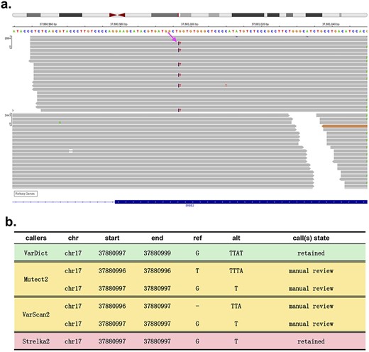
A complex multinucleotide variant at chr17:37880997 in the human reference genome hg19. (A) Integrative Genomics Viewer (IGV) screenshot of reads covering the variant. Each read is represented by a grey bar. The purple vertical lines on reads represent insertion events, and the different bases are coloured. For example, the red ‘T’ represents a single-nucleotide variant (SNV) from G to T. (B) Calls of VarDict, Mutect2, VarScan2 and Strelka2.
An effective strategy for improving the accuracy of variant detection is to integrate the variants called by multiple callers, for instance, adopting the union or intersection of results from various callers for SNVs and selecting indels that are called by at least two of three callers to ensure a higher accuracy [54]. Open-source callers based on this idea are already available, such as CAKE and GenomeVIP [4, 55].
Although filtering variants cannot remedy true-negatives, some strategies can be conducted to reduce the number of false positives. Most variant callers have corresponding filtering methods; not all methods are suitable for particular studies. This has been observed in the case of GATK’s Variant Quality Score Recalibration (VQSR), which uses at least 5000 variants that coincide with a known mutation set (HapMap) to train a Gaussian mixture model and then distinguishes true variants from false positives [56]. Variants from WGS or WES (of region size of at least 50 M) data work well; however, anything smaller, such as that from gene-panel sequencing, may encounter difficulties or errors. Similarly, the best practice of somatic SNV and indel calling in GATK introduces ‘panel of normal’ (PON), which requires blood samples from at least 40 healthy young people. Furthermore, the most critical selection criteria for ‘normals’ are technically similar to those of tumours (same exome or genome preparation methods and sequencing technology). The rigorous standards of running VQSR and building a PON pose significant challenges to research in small- to mid-sized laboratories. Therefore, although we recommend using multiple callers to detect variants, we strongly discourage filtering false positives using a crossover method.
In this study, we also performed the mutual verification between variant callers for tumour samples without matched controls (Figure 2B), revealing a dramatically high false-positive rate and indicating that variant detection in an individual tumour sample requires more work and exploration.
The focus of QC during variant calling is the heterozygosity/homozygosity ratio, transition/transversion (Ti/Tv) ratio and mutation load, which help understand variants from a sample level. For WGS data, the heterozygosity/homozygosity ratio for variants in Hardy-Weinberg equilibrium is 2.0, with a striking bias indicating errors such as unpaired tumour-normal samples [31]. The Ti/Tv ratio which is approximately 3.0 for SNVs in exons and around 2.0 for non-exons is another QC indicator of overall SNV quality that differs by genomic region [57]. In addition, the mutation number per million bases is an essential indicator of false-positive rates, with Alexandrov showing that the prevalence of somatic mutations varies from 0.001 to over 400 per million bases between and within cancer categories with adequate samples [58].
Currently, there are only a few analysis tools that comprehensively focus on variant calling QC for different applications and purposes; however, many variant callers provide modules for checking certain aspects. For example, a module named ‘Calculate Contamination’ in GATK 4.0 provides fractional contamination to inform downstream filtering, whereas SnpEff, QC3 and VariantQC in NGS-Bits are tools for profiling variant quality that provide the Ti/Tv and non-reference homozygosity ratios as well as cross-sample contamination checks [9, 59, 60]. Picard provides modules processing VCF files such as FixVcfHeader, MergeVcfs and SortVcf. In addition, NGSCheckMate can achieve faster sample consistency checking using VCF files. However, VCF files must be generated by variant callers; if sample mismatches are found in the calling stage, the previous processing steps make no sense but are a waste of resource, especially the multi-step alignment and variant calling which cost much time and storage. Therefore, although FASTQ and VCF files can also be used to detect sample consistency, applying BAM files is a compromise strategy which can not only save time but also find mismatches as early as possible to avoid dirty work.
Variant annotation and visualisation
Variant annotation is the aggregation and summarisation of data relevant to a candidate genomic alteration and is a crucial step in cancer genome sequencing that is crucial for the ultimate prediction of functional effects. Importantly, variant annotation can decipher variants from miscellaneous aspects of basic information (such as gene symbols and functional classification) to disease-specific predictions and drug sensitivity derived from databases to pinpoint a small subset of potential disease-causing mutations for further interpretation.
Genetic variant databases of large-scale populations, such as 1000 Genomes, GnomAD (The Genome Aggregation Database), ESP6500 (NHLBI GO Exome Sequencing Project v. 6500) and ExAC (Exome Aggregation Consortium) aggregate populations and allele frequency, allowing investigators to distinguish somatic mutations from germline variations [61–64]. GnomAD contains WGS samples from more than 15 496 individuals and WES samples from over 123 316 individuals and is currently recognised as the most significant genetic variant research database. Databases associated with genetic diseases include ClinVar, HGMD (The Human Gene Mutation Database) and OMIM (Online Mendelian Inheritance in Man). ClinVar is a freely accessible archive of relationships between human genome variations and phenotypes with evidence from expert reviews [65–67], whereas HGMD collates all published gene lesions related to human inherited disease from approximately 250 journals. OMIM contains mutations identified in published materials from research worldwide. COSMIC (Catalogue of Somatic Mutations in Cancer) contains variants related to human cancer and is currently the most comprehensive expert-curated global dataset for exploring the effect of somatic mutations on cancer. In addition, prediction tools such as SIFT, PolyPhen2, GERP++, CADD and REVEL are used to evaluate the malignancy and pathogenicity of missense variants [68–72]. Table 2 summarises the commonly used databases and prediction tools that facilitate access to and communication about variation and disease.
Databases and predictors used in annotations
| Databases or software | Name | Public | Samples or variants | Type | URL | |
|---|---|---|---|---|---|---|
| Frequency database | For variant frequency in WGS | 1000 Genomes: The 1000 Genomes Project dataset [61] | Yes | ~84.40 million variants from 2504 samples | WGS | http://www.internationalgenome.org/data |
| Kaviar: Known VARiants [73] | Yes | ~170.00 million variants from 77 781 samples | ~132 000 WGS, ~644 000 WES | http://db.systemsbiology.net/kaviar/ | ||
| Haplotype Reference Consortium database [74] | Yes | ~40.00 million variants from 32 000 samples | Panels | http://www.haplotype-reference-consortium.org/ | ||
| 69 Genomes Data: Allele frequency in 69 human subjects | Yes | 69 samples | WGS | https://www.completegenomics.com/public-data/69-genomes/ | ||
| gnomAD: The Genome Aggregation Database [62] | Yes | 138 632 samples | 15 496 WGS | https://macarthurlab.org/2017/02/27/the-genome-aggregation-database-gnomad/ | ||
| For variant frequency in WES | gnomAD: The Genome Aggregation Database (gnomAD) [62] | Yes | 138 632 samples | 123 136 WES | https://macarthurlab.org/2017/02/27/the-genome-aggregation-database-gnomad/ | |
| ESP6500: NHLBI GO Exome Sequencing Project v. 6500 [63] | Yes | 6503 samples | WES | http://evs.gs.washington.edu/EVS/ | ||
| ExAC: Exome Aggregation Consortium dataset [64] | Yes | 60 706 samples | WES | http://exac.broadinstitute.org/ | ||
| Functional prediction tools | For functional variant prediction in WGS | (Software) GERP++: Genomic Evolutionary Rate Profiling [70] | Yes | ~9.00 million variants | WGS | http://mendel.stanford.edu/SidowLab/downloads/gerp/ |
| (Software) CADD: Combined Annotation Dependent Depletion [71] | Yes | ~9.00 million variants | All | https://cadd.gs.washington.edu/ | ||
| (Software) DANN: A deep learning approach for annotating the pathogenicity of genetic variants [75] | Yes | — | All | https://dbpia.nl.go.kr/bioinformatics/article/31/5/761/2748191 | ||
| (Software) Fathmm: Functional Analysis Through Hidden Markov Models [76] | Yes | ~9.00 million variants | Coding and noncoding | http://fathmm.biocompute.org.uk/ | ||
| (Software) EIGEN: A spectral approach integrating functional genomic annotations for coding and noncoding variants [77] | Yes | ~9.00 million variants | Coding and noncoding | http://www.columbia.edu/~ii2135/eigen.html | ||
| (Software) GWAVA: Eigen scores [78] | Yes | — | Noncoding | https://www.sanger.ac.uk/science/tools/gwava | ||
| For functional variant prediction in WES | dbNSFP: An annotation database for assembled non-synonymous SNPs [79] | Yes | — | WES | https://sites.google.com/site/jpopgen/dbNSFP | |
| For functional splice variant prediction | scsnv: A likelihood score that a variant affects splicing [80] | Yes | — | Splicing | https://www.ncbi.nlm.nih.gov/pmc/articles/PMC4267638/ | |
| SPIDEX: Splicing Index [81] | Yes | — | Splicing | http://tools.genes.toronto.edu/ | ||
| Disease database or tools | For disease-specific variants | ClinVar: Clinical Variants [65] | Yes | ~0.43 million variants | Coding | https://www.clinicalgenome.org/data-sharing/clinvar/ |
| COSMIC: The Catalogue of Somatic Mutations in Cancer [82] | Yes | ~3.00 million variants | Coding and noncoding | https://cancer.sanger.ac.uk/cosmic/ | ||
| ICGC: International Cancer Genome Consortium | Yes | ~68.00 million variants | Coding | https://icgc.org/ | ||
| For variant identifiers | dbSNP: The NCBI database of genetic variation [83] | Yes | ~60.00 million variants | WGS | https://www.ncbi.nlm.nih.gov/snp/ | |
| OMIM: Online Mendelian Inheritance in Man [67] | No | ~0.03 million variants | WGS | https://omim.org/ | ||
Currently, there are four leading tools used to annotate DNA variants: Annovar, SnpEff, VEP (Variant Effect Predictor) and Oncotator (Table 3) [59, 84–86]. Annovar can flexibly annotate SNVs or SNPs, indels and CNVs according to continuously updated publicly available resources and user-contributed datasets. Also, Annovar annotates variants by gene-based, region-based and filter-based methods and can handle gene definitions from RefSeq, UCSC, Ensembl and GENCODE. Moreover, Annovar can accept variants in VCF as input and convert variant lists in VCF into a specific format using its internal scripts.
Annotators for variant annotation
| Annotator | Language | Human reference genome | Input format | Output format | Prepare input function | Download database function | Self-build database | Filtering function | Statistics filtering | Variant type | Web-interface |
|---|---|---|---|---|---|---|---|---|---|---|---|
| VEP | Perl | GRCh38(HG38)/GRCh37(hg19) | VCF | VCF | χ | ✓ | ✓ | ✓ | χ | SNVs;indels;CNVs;SVs | χ |
| Oncotator | Python | GRCh37(hg19) | VCF;TCGAMAF;MAFLITE | VCF;MAFLITE | χ | χ | ✓ | χ | χ | SNVs;indels | ✓ (http://www.broadinstitute.org/oncotator) |
| SnpEff | Java | GRCh38/GRCh37(hg19) | VCF | VCF | ✓ | ✓ | χ | χ | ✓ | SNVs;indels | χ |
| Annovar | Perl | GRCh38/GRCh37(hg19) | VCF; Annovar input | VCF; Annovar output | ✓ | ✓ | ✓ | ✓ | χ | SNPs; indels;CNVs | ✓ (http://asia.ensembl.org/Tools/VEP) |
Meanwhile, Oncotator integrates data from 14 public resources to annotate SNVs and indels with data relevant to cancer studies and has been used in the Broad Institute’s Cancer Genome Analysis pipeline; thus it is crucial for several large-scale projects conducted by TCGA, NHGRI and TARGET. Oncotator is also available as a python module for local use and is accessible as a web service that can deal with multiple input formats, including VCF, TCGAMAF (mutation annotation format) and MAFLITE. However, due to its processing of the ‘INFO’ field, the MAF files generated from the VCF files of various callers (such as VarDict and GATK) display different column titles, column numbers and column order [87]. Thus, to ensure the consistency of the annotation results, variants in VCF need to be converted into the MAFLITE format, requiring additional manual scripts. Oncotator only supports the GRCh37 (hg19) human reference genome, and no update has been released for over 3 years.
SnpEff is a toolbox that performs genetic variant annotation and functional effect prediction, whereas SnpSift manipulates the variants annotated by SnpEff, thus filtering large genomic datasets and identifying the most significant variants. ClinEff is an innovative tool released as a professional version of the SnpEff and SnpSift suites and is more suitable for clinical uses and production operations [88, 89]. However, ClinEff suites only process VCF input files and produce VCF files with a new field, ‘ANN’, while requiring additional configuration before annotation which may require professional IT knowledge.
Lastly, VEP annotates SNPs, indels, CNVs and SVs (structural variants) by providing up to 32 variant classifications and the corresponding filtering or statistical scripts. VEP also reads both compressed (gzipped) and uncompressed input files of multiple formats, such as VCF and HGVS identifiers, and returns annotations in tab-delimited, VCF and JSON formats. Simultaneously, VEP generates an HTML file containing statistics on the annotation results, presenting a general report of command line parameters, running time and information about the number of variants, genes, transcripts and regulatory features overlapped by the input variants.
Due to the different algorithms, transcripts and reporting strategies, the results of various annotation tools differ significantly in their transcript and genome features. For instance, VEP reports all possible transcripts, whereas Annovar only returns the transcripts with the most severe consequence according to its internal precedence, as demonstrated by McCarthy et al. [90]. We, therefore, recommend utilising VEP to annotate tumour-normal paired cancer genome variants due to its advantage of filtering scripts suite and providing a statistical report and then utilize Vcf2maf converting variants in VCF to TCGA MAF [91], which is often required by many subsequent software such as MuSiC2 for detecting significantly mutated genes, MutSigCV for identification of driver genes and Hotspot3D for determining protein structure [92–94].
The visual inspection of aligned reads to validate and interpret candidate variants is an essential aspect of cancer genome sequencing. Visualisation tools display aligned reads with mapping characteristics (e.g. mapping quality, depth, strand) and variants with annotation information from various databases in a user-friendly, smooth, intuitive and responsive method. We have divided the most prevalent visualisation tools into web servers and stand-alone applications. Ensembl Genome Browser, JBrowse Genome Browser, UCSC Genome Browser and VEGA Genome Browser are web servers that display the uploaded data in the context of online resources while avoiding the hassle of downloading and complex installation [95–98]. These servers can deal with user-defined tracks by either uploading a file or specifying a remote URL; however, they require additional data handling such as indexing and sorting files into a fixed format that may be difficult for inexperienced practitioners. Due to limitations such as network bandwidth, cybersecurity and privacy issues with respect to uploading large sequence data, web-based visualisation tools are more suitable for temporarily viewing data in a small region of interest or exploring published datasets included in public databases. Conversely, Artemis, IGV (Integrative Genomics Viewer) and Savant (Sequence Annotation and Visualisation and Analysis Tool) are stand-alone visualisation tools that can flexibly display variants with interactive browsing and zooming features [99–101]. Although there is no need to access large volume data remotely, these methods do require that annotation resources are downloaded and updated to allow meaningful visualisation and validation. In addition, the high memory and computing requirements for large volume data such as WGS samples require computers or clusters equipped with large memory and storage. Thus, stand-alone visualisation tools are suitable for experienced analysts with an IT background viewing sequence data in large-scale clinical cancer sequencing.
Conclusion and discussion
The process of translating obscure cancer genomic data to clinical practice involves a series of large and complicated steps, including foundational analysis to detect variants, advanced interpretation to reveal molecular profiles and multi-omics approaches to obtain biological insights. We limited this review to foundational analysis, an interdisciplinary area of bioinformatics and computer science, and conducted a comprehensive and systematic investigation of the tools, strategies and published literature regarding cancer genome sequencing, emphasising the importance of QC in each step. Although we investigated and compared many tools for cancer genome sequencing, other aspects, such as sample extraction, library preparation and sequencing processes, are of equal importance. Here, we limited the study to the analyses of sequencing data from Illumina sequencers. QC should be applied in each step of the cancer genome sequencing data analysis, i.e. raw data pre-processing, alignment, variant calling and annotation in different resolutions from a single sample, the cohort level (Figure 1). The recommendations we proposed will serve as valuable guidelines for both skilled and inexperienced practitioners in making decisions regarding the appropriate tools and optimal steps for specific applications, with the anticipation of promoting the development of precision medicine.
Open-source software, workflows and public resources have greatly boosted the mining of cancer genomes; however, there are a variety of tools available for each step of the analysis that can handle a diverse range of genomic data formats (FASTQ, BAM, SAM, VCF, MAF) and are attracting increasing attention to be more widely used in routine analysis. This is illustrated by some of the tools discussed in this review; for instance, NGSCheckMate validates sample identity from FASTQ, BAM and VCF input files and is effective for different data types (WES, WGS and RNA-seq), whereas VarDict detects a wide range of variant signals including SNVs, indels, CNVs and SVs with a single scan of aligned sequences. Similar tools with versatile features also include NGS-Bits, MultiQC and IGV.
There are several other aspects that can potentially influence cancer genome sequencing. Firstly, the entire foundational analysis of genomic data is a coherent process, wherein the results of the first step directly affect the accuracy of subsequent procedures. Therefore, tool developers should provide not only the functions and features of their own tool but also compatibility with upstream tools. Secondly, test datasets (such as NA12878) with various characteristics, ground truth and filtering standards sequenced from real samples should be improved or released to provide uniform and objective evaluation criteria. Thirdly, large-scale studies should aim to eliminate imbalanced population diversity in public databases as Landry et al. found significantly fewer studies in the Asian (29%) and other populations (4%; e.g. African and Latin American) than European populations (67%) [102]. Cancer genome sequencing relies on population-based resources to remove common genomic polymorphisms; therefore, population imbalance may have little effect on cancer investigations in underrepresented populations. However, it is necessary to establish genomic polymorphism databases in specific populations.
Several popular pipelines or software in cancer genome sequencing data analysis cannot be used in all applications and should be selected based on specific research needs.
Local realignment step is very critical in the whole pipeline, but whether this step should be performed depends on the variant caller chosen in the next step.
Quality control should be conducted in each step using appropriate software to ensure accuracy of the analysis.
Funding
National Natural Science Foundation of China (grant number 31771466); National Key R&D Program of China (grant numbers 2018YFB0203903, 2016YFC0503607, and 2016YFB0200300); Special Project of Informatization of the Chinese Academy of Sciences, China (grant number XXH13504-08).
Conflict of interest
The authors have declared that no conflict of interests exist.
Xiaoyu He, Ph.D., Computer Network Information Center, Chinese Academy of Sciences; University of Chinese Academy of Sciences, is mainly engaged in cancer genomics research and construction of the Chinese cancer genome database.
Shanyu Chen, Computer Network Information Center, Chinese Academy of Sciences; University of Chinese Academy of Sciences, Beijing 100190, China.
Ruilin Li, Computer Network Information Center, Chinese Academy of Sciences; Beijing 100190, China.
Xinyin Han, Computer Network Information Center, Chinese Academy of Sciences; University of Chinese Academy of Sciences, Beijing 100190, China.
Zhipeng He, Computer Network Information Center, Chinese Academy of Sciences; University of Chinese Academy of Sciences, Beijing 100190, China.
Danyang Yuan, Computer Network Information Center, Chinese Academy of Sciences; University of Chinese Academy of Sciences, Beijing 100190, China.
Shuying Zhang, Computer Network Information Center, Chinese Academy of Sciences; University of Chinese Academy of Sciences, Beijing 100190, China.
Xiaohong Duan, ChosenMed Technology (Beijing) Co., Ltd., Beijing 100176, China.
Beifang Niu, Computer Network Information Center, Chinese Academy of Sciences; University of Chinese Academy of Sciences, Beijing 100190, China; ChosenMed Technology (Beijing) Co., Ltd., Beijing 100176, China.
