


Abstract
Metaproteomics suffers from the issues of dimensionality and sparsity. Data reduction methods can maximally identify the relevant subset of significant differential features and reduce data redundancy. Feature selection (FS) methods were applied to obtain the significant differential subset. So far, a variety of feature selection methods have been developed for metaproteomic study. However, due to FS’s performance depended heavily on the data characteristics of a given research, the well-suitable feature selection method must be carefully selected to obtain the reproducible differential proteins. Moreover, it is critical to evaluate the performance of each FS method according to comprehensive criteria, because the single criterion is not sufficient to reflect the overall performance of the FS method. Therefore, we developed an online tool named MetaFS, which provided 13 types of FS methods and conducted the comprehensive evaluation on the complex FS methods using four widely accepted and independent criteria. Furthermore, the function and reliability of MetaFS were systematically tested and validated via two case studies. In sum, MetaFS could be a distinguished tool for discovering the overall well-performed FS method for selecting the potential biomarkers in microbiome studies. The online tool is freely available at https://idrblab.org/metafs/.
Introduction
Microbial community (MC) exists widely in nature and plays an irreplaceable role in the ecological system [1], agricultural production [2], industrial manufacture [3] and human health [4–6]. The OMIC-based studies on MC have been carried out for many years [7, 8] to explore species evolutions [9], define taxonomic hierarchy [10, 11], investigate disease-relevant gene [12, 13] and discover new biomarkers, targets or drugs [14–19]. OMIC technologies are developing rapidly [20]; among different OMIC technologies, metaproteomic has emerged to be one of the hottest research field, which provides invaluable insights into (1) the understanding of MC and its interaction with the host environment [21], (2) the identification of MC structure and function during urinary tract infections [22] and (3) the exploration of drug-resistant traits in bacteria [15, 23]. Moreover, the significant changes in the protein abundance of certain bacterial species have been reported as linked to many complex diseases, for example, inflammatory bowel diseases [24].
However, the reliability of these findings depends on the applied computational approaches in these studies [25–30]. As reported, metaproteomic data suffered from two inevitable problems: sparsity and dimensionality [31, 32]. The solution to the issues of dimensionality in metaproteomic data is the usage of data reduction methods. Moreover, identification of specific proteins in metaproteomic is not always easy. In particular, the low efficiency of microbial protein identification [33] is the key difficulty in metaproteomic, and this may attribute to the enormous diversity and individual variations of microbiome and the lack of a suitable database for peptide-spectra matching [33]. The general strategy is to utilize feature selection (FS) methods to reduce the data dimensionality effectively. As for the protein identification redundancy caused by homologous proteins, it could be reduced by grouping proteins according to sequence similarity [34] or shared peptides [35]. As reported, these expected FS methods can maximally identify the relevant subset of significantly differential features [36] and eliminate data redundancy [31]. Therefore, in order to extract the specific subset successfully, an appropriate differential abundance analysis must be employed in microbiome proteomics studies [37]. So far, varieties of feature selection (FS) methods have been proposed to identify the difference of proteins abundance between the case and control group [25, 38, 39]. Over the past few years, more than 13 FS methods have been established for the analysis of metaproteomic data based on mass spectrometry (MS).
Because the theories behind each statistical selection method varied greatly, and performance of methods depended heavily on the data characteristics, the strategies used for feature selection must be selected carefully in data analysis [25, 40]. Thus, it is practical and necessary to distinguish the best method from other methods when analyzing a particular dataset [25]. However, due to the different focus of each criterion, a single criterion is not sufficient to accurately assess the performance of these FS methods. It is recommended to comprehensively consider multiple criteria and evaluate each method’s performance from different perspectives. So far, there are four available well-established criteria, including (a) method’s clustering performance based on the identified significant changes in proteins abundances [41]; (b) method’s robustness based on the identified significantly differential peptides/proteins among multiple datasets [27]; (c) method’s predictive accuracies based on the supervised classification models [42, 43] and (d) method’s capability of identifying the true positive markers based on the spiked microbial proteins [25, 44, 45]. In a word, the evaluation of FS methods’ performance via multiple criteria is essential to choose the well-performed one for biomarker discovery.
A number of tools are available for metaproteomic data analysis, such as MicrobiomeAnalyst [46], MetaComp [47], iMetaLab [21], MetaProteomeAnalyzer [48] and Galaxy framework [49]. iMetaLab, MetaProteomeAnalyzer and Galaxy framework mainly focused on constructing the specific-sample database, peptide/protein identification and quantification and taxonomic and functional annotation in metaproteomic data analysis but can’t provide the statistical methods for identifying significant changes in bacterial species abundance. Only the MicrobiomeAnalyst and MetaComp can perform metaproteomic statistical data analysis to identify proteins with differential abundance [46], but they have no function to evaluate the performance of statistical methods. Moreover, for the basic statistical analysis software for proteomic, such as SPSS [50] and PAST [51], they cannot provide a complete workflow of data processing and performance evaluation of FS method, which leads to their limitations on selecting the superior FS methods in metaproteomic research. In addition, a single criterion is not sufficient to reflect the overall level of the FS method due to the nature of complex metaproteomic dataset [25]. Thus, in order to identify more effective biomarkers in metaproteomics, there is now an urgent need to provide a user-friendly service in metaproteomic data analysis for comprehensively evaluating these statistical methods, which can improve the efficiency of identifying the differential abundance proteins in bacterial species.
In this work, we developed a web server for not only identifying the differential abundance proteins between two distinct groups but also fully assessing the applicability of different FS methods from different perspectives. MetaFS is freely available at the website (https://idrblab.org/metafs/). MetaFS could utilize 13 FS methods for selecting significant features and provide results of performance evaluation by comprehensively considering four different criteria. Moreover, two case studies in the last section of the article demonstrated the innovativeness and practicability of the new service. In summary, MetaFS aims to distinguish the well-performed feature selection method from other methods based on multiple criteria and identify robust and reliable potential biomarkers. MetaFS could provide a useful guidance for selecting appropriate statistical method for metaproteomic biomarkers discovery.
Materials and methods
Feature selection methods analyzed in this study
In this study, 13 FS methods for biomarker discovery of MS-based metaproteomics were analyzed, which contained (1) chi-square, (2) correlation-based feature selection, (3) entropy-based filters, (4) fold change, (5) linear models and empirical Bayes, (6) partial least squares discriminant analysis, (7) orthogonal partial least squares discriminant analysis, (8) relief, (9) random forest recursive feature elimination, (10) significance analysis for microarrays, (11) support vector machine recursive feature elimination, (12) univariate t-test and (13) Wilcoxon rank-sum test. As previously reported, the assumption of normality should be checked for some specific FS methods [52]. In other words, the pretreated data should be tested for normal distribution before selecting some FS methods [52]. The quantile–quantile (QQ) plot is a widely accepted visually method for normality test [53] and can be applied in this study before choosing FS methods. Table 1 demonstrates the categories of these feature selection methods according to the assumption, type and advantage. According to these categories, 13 feature selection methods were grouped in the interface of step 4 in the MetaFS. The detailed descriptions of 13 FS methods including their requirements for data structure are provided in the Supplementary data.
The characteristics of each feature selection method according to the assumption, type and advantage. All feature selection methods are categorized by assumption and type and listed alphabetically
| Full Name | Abbr. | Assumption | Type | Advantage |
|---|---|---|---|---|
| Chi-square | CHIS | Non-normality | Univariate filter | Calculation is simple |
| Independent of classifier | ||||
| Fold change | FC | Non-normality | Univariate filter | Calculation is simple |
| Independent of classifier | ||||
| Significance analysis of microarrays | SAM | Non-normality | Univariate filter | Calculation is simple |
| Independent of classifier | ||||
| The Wilcoxon rank-sum test | Wilcox | Non-normality | Univariate filter | Calculation is simple |
| Independent of classifier | ||||
| Linear models and empirical Bayes | LMEB | Normality | Univariate filter | Calculation is simple |
| Independent of classifier | ||||
| Univariate t-test | t-test | Normality | Univariate filter | Calculation is simple |
| Independent of classifier | ||||
| Correlation-based feature selection | CFS | Non-normality | Multivariate filter | Models feature dependency |
| Independent of classifier | ||||
| Computation is complexity | ||||
| Relief | REF | Non-normality | Multivariate filter | Models feature dependency |
| Independent of classifier | ||||
| Computation is complexity | ||||
| The entropy-based filters | ENTROPY | Non-normality | Multivariate filter | Models feature dependency |
| Independent of classifier | ||||
| Computation is complexity | ||||
| Orthogonal partial least squares discriminant analysis | OPLS-DA | Normality | Multivariate filter | Models feature dependency |
| Independent of classifier | ||||
| Computation is complexity | ||||
| Partial least squares discriminant analysis | PLS-DA | Normality | Multivariate filter | Models feature dependency |
| Independent of classifier | ||||
| Computation is complexity | ||||
| Random forest recursive feature elimination | RF-RFE | Non-normality | Embedded | Models feature dependencies |
| Interacts with the classifier | ||||
| Good predictive model for high-dimensional data | ||||
| Support vector machine recursive feature elimination | SVM-RFE | Non-normality | Embedded | Models feature dependencies |
| Interacts with the classifier | ||||
| Good predictive model for high-dimensional data |
Four criteria for evaluating performance of feature selection methods in this study
Compared with the previous publication on the assessment of FS methods [27], two new and widely accepted criteria (unsupervised clustering performance and robustness performance between features identified) were further added in this study. In total, MetaFS integrated four independent criteria to assess the performance of FS methods.
(a) Method’s unsupervised clustering performance of the identified significantly differential peptides/proteins [54–56]. An appropriate FS method was supposed to preserve or sometimes enlarge the difference in proteomics dataset in two different groups [57]. Based on protein intensities of samples, the unsupervised hierarchically clustering (visualization via heatmap) was therefore frequently applied as an effective metric [57]. In hierarchical clustering analysis, the Manhattan and Euclidean distances were widely applied for estimating the similarity among the samples [58]. Euclidean is the most commonly used distance measurement which can calculate the root of square differences between protein abundances of a pair of samples, while the Manhattan distance calculates the absolute abundance differences. The types of both clustering methods were provided in the MetaFS. Moreover, the heatmap was employed to illustrate the result of clustering analysis. Specifically, the cell with the highest abundance value was set to red and those lower abundance values gradually fading toward green. First, feature selection methods reduced the whole number of proteins studied. Then, these selected markers were reused to perform hierarchical clustering of samples and proteins, resulting in a two-way clustering diagram in which columns (samples) and rows (proteins) are clustered via their similarities in protein intensity profile. The FS method will be considered well-performed under this criterion when there is an obvious separation between two group samples on the heatmap, that is, the red module and the green module are separated obviously. This criterion highlights the clustering performance and is an embodiment of the effectiveness of methods [59].
(b) Method’s robustness of the significantly differential peptides/proteins among multiple datasets [55, 60]. In this criterion, Venn diagram was employed to illustrate the numbers of the overlapped differential proteins. With the help of this criterion, we defined consistency score [55] to characterize the common part of the identified markers in various sections of available data quantitatively. In the identification of markers for given data, with a higher consistency score, it could represent the results to be more robust. The evaluation results of this criterion can reflect the universality of the selected FS method [55] and the reproducibility of identified significantly differential markers [61].
(c) Method’s predictive accuracies based on the supervised classification models [54, 56, 59, 62]. In this case, on the basis of support vector machine (SVM), the area under the curve (AUC) as well as the curve of receiver operating characteristic (ROC) [63–65] was provided. First, differential abundance features are identified by each FS method based on the processed dataset. Secondly, based on these identified features, the SVM models are then constructed. The output of this evaluation criteria is a graph whose x-axis was named as ‘Specificity’ and y-axis was named as ‘Sensitivity’. The specificity represents the true negative rate and the sensitivity refers to the true positive rate. The higher these two values, the better the FS method.
(d) Method’s capability of identifying the true positive markers. As reported, an expected FS method is supposed to screen the full list of differential features relevant to the spiked proteins [66–68]. Thus, the optimal feature set derived from the differential abundance proteins could be applied for measuring each algorithm’s ability on identifying the true positive markers. The ideal set of features should only include features relevant to spiked proteins (true positives). These differential features based on each FS method contain spiked features (true positives) and non-spiked compound-related features (false positives). Then, the number of identified spiked proteins was counted for uncovering the performance of the method [25] and the identification rate of spiked proteins (IRSP) was calculated, whose formula is the number of true spiked proteins identified/the total number of true spiked proteins. IRSP is the most intuitive value, and you can just refer to its value. The FS method with higher IRSP value is reasonably expected to perform better.
Every criterion as well as their relevant measures described above was offered in the MetaFS. Multiple combinations of the criteria may offer a more comprehensive assessment on the FS methods. The results of evaluation of all criteria could be directly displayed and be completely downloaded from the online tool.
Implementation details of the MetaFS tool
The MetaFS was developed on a server equipped with a RAM of 128GB and a CPU E7–4820 × 32 cores which ran the operating system of Cent OS Linux v7.0. In addition, the interface of tool was set up by applying R v3.5.0 and the R/Bioconductor package Shiny which ran on the Shiny Server v1.5.3.838. A variety of R/Bioconductor packages were integrated in the implementation, which included affy, AUC, DiffCorr, d3heatmap, DT, e1071, FSelector, fastlo, impute, ggsci, limma, metabolomics, mixOmics, corrplot, ropls, varSelRF, vsn and so on. Users could easily access MetaFS without any log in requirement via various browsers.
Required input files of MetaFS
The required file is supposed to provide a matrix of sample feature in a format of csv (the input format of PXD002099 is shown in Figure S1a in the Supplementary data). In input file, the unique sample ID as well as the corresponding label information must be listed at first two columns of the required file and kept as ‘SampleName’ and ‘Label’, respectively. The peptide/protein’s abundances across all the samples do not need to be log scaled, and the peptide/protein’s unique ID must be listed on the first row of the input file. Particularly, the correct format of input file can be easily produced using popular quantification software (e.g. MaxQuant). An example file named ‘MetaFS_Unified_Data’ could be downloaded directly from the first ‘HERE’ link under the ‘Upload Quantification Data’ pattern in the first step of MetaFS’s ‘Analysis’ module.
In order to assess the capability of identifying the true positive markers, another specific file is required for further analysis (the input format of PXD002099 is shown in Figure S1b in the Supplementary data). In this file, users only need to provide the concentration matrix of the spiked proteins in samples. All the samples in this file have spiked proteins, and the sample IDs as well as the corresponding classes are requested at the first two columns, whose annotation were ‘Sample ID’ and ‘Label’, respectively. Importantly, the samples should be labeled in two different conditions. Also, the first row must provide the unique IDs of all the spiked proteins. An example file named ‘unified_metafs_gold’ could also be obtained from the second ‘HERE’ link under the ‘Upload Quantification Data’ pattern in the first step of MetaFS’s ‘Analysis’ module.
Output files of MetaFS
The output files included (1) histograms, boxplots and QQ plots before and after pretreatment, (2) a variety of statistical results (.png and .csv) of the significantly differential features via each FS method and (3) various evaluation results on the performance of each FS method via four independent criteria (e.g. Venn diagrams, unsupervised hierarchical clustering, ROC curve and so on). The all resulting files and performance assessment documents in the specific format (.png and .csv) are also downloadable from MetaFS’s ‘Analysis’ page directly. An exemplar output file with evaluation results via each criterion could be downloaded from MetaFS’s ‘Tutorial’ page.
Case studies of MetaFS based on two benchmark datasets
The MetaFS could accept peptide/protein quantification data generated by various popular software (e.g. MaxQuant, Progenesis QI, PEAKS and Scaffold). In this study, two representative metaproteomic benchmark datasets (PXD006224 and PXD002099) were collected for testing and validating the function of MetaFS (Table 2). These datasets were collected from PRoteomics IDEntifications (PRIDE) database [69]. The experimental data including the spiked proteins is very suitable to serve as a reference to validate performances of FS method, because the spiked-in proteins are truly different. FS methods are evaluated based on the number of spiked proteins identified by each FS method. Thus, the PXD002099 dataset containing the spiked proteins was collected to achieve the above purposes. In addition, because of the small number of samples in PXD002099 (3 versus 3), the dataset with larger sample size (PXD006224) was collected to assess consistency among varied feature sets derived from the various sampling datasets.
The spiked proteins and non-spiked proteins benchmark microbial proteomic datasets collected for the analysis of this study. These datasets were collected from PRIDE database
| Datasets | Dataset ID | Dataset description | No. of features | Quantification software tool |
|---|---|---|---|---|
| J Proteome Res. 14:4118–26, 2015 | PXD002099 | Digested UPS1 mixture was spiked into a yeast proteome digest to create five UPS1 concentrations (2, 4, 10, 25 and 50 fmol/μl), 3 runs per spiked concentration [48 spiked proteins] | 1442 | Progenesis |
| Microbiome. 5:144, 2017 | PXD006224 | 60 metabolic phase fecal samples 24 equilibrium phase fecal samples | 9161 | MaxQuant |
Based on above two benchmark datasets, two case studies were conducted, which included (case study 1) comprehensive evaluation of the performance of FS methods on the basis of dataset PXD006224 and (case study 2) assessment of FS methods’ performance based on the spiked-in proteins of PXD002099.
In case study 1, PXD006224 [70] comprised 60 ‘metabolic phases’ fecal samples as well as 24 ‘equilibrium phases’ fecal samples. In total, 9161 proteins were measured for each sample by the MaxQuant software. This dataset with the large sample size was well-suited for assessing consistency among varied feature sets derived from the various sampling datasets [71, 72].
In case study 2, PXD002099 [73] provided information on the true difference between two distinct groups, which was quantified by Progenesis QI software. In particular, 48 UPS1 (universal proteomics standard 1) proteins were spiked into the background proteome with the five different levels of concentration, and each concentration has three replicates conducted via LC-MS platform. To construct a dataset with truly differential proteins between two distinct groups for evaluating performance of FS methods on detecting truly differential proteins, each sample was divided into two categories of the different concentrations of the spiked proteins by combining with each other. In sum, all samples were divided into 10 different datasets by combining with each other. In particular, the ‘low versus high’ concentrations (fmol/μl) of the spiked proteins were 2 versus 4, 2 versus 10, 2 versus 25, 2 versus 50, 4 versus 10, 4 versus 25, 4 versus 50, 10 versus 25, 10 versus 50 and 25 versus 50, respectively.
Moreover, in order to evaluate and select the appropriate FS method for the specific data, it is necessary to upload each quantitative dataset multiple times for generating results based on the different FS methods. Specifically, the analysis procedure included uploading the quantification data, selecting the specific pretreatment methods, selecting the specific imputation methods, choosing the specific feature selection, evaluating the performance of the selected workflow and downloading the corresponding evaluation outputs. As reported, the variance stabilization normalization (VSN) can reduce variations between samples and was identified as well-performed pretreatment method in the analysis of differential abundance [44], and it was applied to pretreat these two benchmark datasets before feature selection in this study. After VSN processing, QQ plot showed that the distributions of the two benchmark datasets were normal in this study, which indicated that all the 13 FS methods studied could be applied to these two pretreated data. To evaluate the performance of all feature selection methods, the same analysis procedure should be conducted repeatedly, except that the FS method should be selected differently. Subsequently, the performance of the various FS methods was further analyzed.
Results and discussion
Web service and operating procedure of MetaFS
In total, the overall process of MetaFS can be divided into five procedures: (1) uploading raw microbial peptides/proteins quantification dataset, (2) pretreatment of raw dataset and normality test, (3) missing values imputation, (4) identification of differential abundance proteins and (5) evaluating the performance of FS methods. Figure 1 showed the workflow of MetaFS, and the details on how to manipulate and process data using MetaFS could be seen in ‘Tutorial’ page of MetaFS. A user manual, with an example data to show the operation procedure of the software, was provided and available for downloading in the ‘Tutorial’ module of MetaFS.

The general workflow of MetaFS. (A) Uploading the mass spectrometry (MS)-based metaproteomic data with the unified proteins abundances matrix; (B) data pretreatment and normality test; (C) imputation of missing values; (D) differential proteins identified based on feature selection method; (E) performance evaluation by multiple criteria.
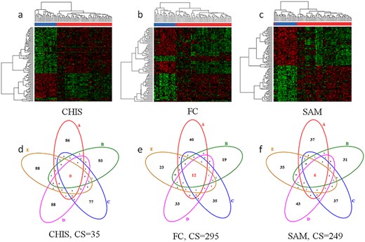
Evaluation results of two criteria on benchmark PXD006224. (1) Method’s clustering performance of the identified significantly differential proteins (heatmap). (a) CHIS’s clustering performance, (b) FC’s clustering performance, (c) SAM’s clustering performance. (2) method’s consistency of the identified significantly differential markers among different datasets (Venn diagram). (d) CHIS’s consistency performance, (e) FC’s consistency performance, (f) SAM’s consistency performance. In heatmap, red indicated control group, and blue represented case group. The Venn diagram demonstrated the number of overlap differential proteins identified based on the five sampling groups (repeating 20 times each group) and the CS indicated the consistency score (the higher the CS value, the better). The number of identified significantly differential proteins was set to 100 for unbiased comparison among feature selection methods.
Step 1: Uploading quantification metaproteomic data
In the step of metaproteomic data uploading, the required file is supposed to provide a matrix of sample feature in the csv format (the input format is shown in Figure S1 in the Supplementary data).
Step 2: Data pretreatment
The pretreatment procedures are required before downstream statistical analysis. Common methods of data pretreatment include transformation, centering, scaling and normalization. Data was often transformed into the log scale [74, 75], which aimed at converting the distribution of peptide/protein intensities into a more symmetric or normal distribution [76]. Centering aimed at converting all the concentrations to fluctuations around zero instead of around the mean of the protein concentrations [74]. Scaling could adjust the fold difference between the detected proteins [74]. Normalization referred to removing the unwanted variations to make individual observations/samples more directly comparable [44, 76]. In total, varieties of pretreatment methods are provided in this procedure, and the detailed information has been provided in a previous study [61]. To provide this information for users, we have created a link named ‘HERE’ in the ‘Step 2. Data pretreatment’ section in ‘Tutorial’ module, which linked to the detailed information (including algorithms) of each pretreatment method.
Moreover, as previously reported, the assumption of normality should be checked for some specific FS methods [52]. Currently, the QQ plot is a widely accepted visually method for testing the normal distribution [53]. Thus, the QQ plot was also provided to allow users to directly perform the normality test in this procedure. If the points in the QQ plot generally fall on the line y = x, it indicates that the unknown distribution conforms to the normal distribution [53].
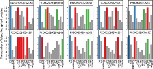
Evaluation results of the number of true positive differential abundance proteins (spiked proteins) on benchmark dataset PXD002099. The performance of each FS method was evaluated based on the number of true positive markers. Each sub-plot demonstrated that the number of true positive markers based on the different concentration pairs. Blue, the top 1 on the performance; red, the top 2 on the performance; green, the top 3 on the performance. UPS1 proteins indicated the true positive markers.
Step 3: Data filtering and missing value imputation
Data filtering and missing value imputation are conducted in this procedure. Data filtering methods could reduce the dimensionality of data [77]. The filtering method used here is the basic filtering, and several imputation methods frequently applied to treat missing value are contained, including the zero imputation, the singular value decomposition (SVD) and the K-nearest neighbor (KNN) methods. By clicking the ‘PROCESS’ button, a summary of the processed data and a plot of the intensity distribution before and after data pretreatment are automatically generated in the ‘Analysis’ page of MetaFS.
Step 4: Identification of differential abundance proteins
In order to obtain differential abundance proteins between two distinct groups, an appropriate FS method must be applied for maximally identifying the relevance and eliminating data redundancy. In sum, 13 FS methods were integrated and provided in the online tool MetaFS, and the detailed instructions on each method could be seen in the ‘Tutorial’ page of MetaFS.
Step 5: Performance assessment of FS from multiple perspectives
Four well-established criteria for comprehensively evaluating the performance of FS method are provided in MetaFS. These criteria included (a) method’s clustering performance of the identified differential features; (b) method’s robustness of selected significantly differential proteins among multiple datasets; (c) method’s predictive accuracies based on the supervised classification models and (d) method’s capability of identifying the true positive markers.
In particular, for criterion (a), the expected clustering analysis based on the differential proteins identified by feature selection method successfully clustered samples according to the studied conditions, whereas distinct samples (control versus case groups) could be visually separated. This indicated that the FS method is quite successful in recognizing the same conditional samples while exposing the differences of distinct condition samples. In criterion (b), the larger overlap number among differential proteins sets among multiple samplings, and the higher consistency score indicated that the FS method generated the more robust differential proteins. In criterion (c), the output is a graph whose x-axis named ‘Specificity’ and y-axis named ‘Sensitivity’. The specificity represents the true negative rate, and the sensitivity refers to the true positive rate. The higher these two values, the better the FS method. In criterion (d), the output included number of identified spiked proteins and the identification rate of spiked proteins (IRSP). The FS method with higher IRSP value is reasonably expected to perform better.
Because of the high cost of parallel computing, this version of the MetaFS is not able to output the performance estimates for all the FS methods at once. Therefore, in order to select the appropriate FS method for the example data in user manual, the quantitative data needed to be uploaded multiple times to generate outputs based on different FS methods. To evaluate the performance of all the FS methods, the same analysis procedure should be conducted repeatedly, except that FS method should be selected differently. Subsequently, the performance of the various FS methods was further analyzed. To the best of our knowledge, the four criteria should be simultaneously considered for selecting the appropriate FS method.
Case study 1: Case studies illustrating inconsistency among different performance assessed by multiple criteria
As reported, several criteria were now suitable for assessing performance of FS methods. These criteria included classification capacity based on the unsupervised clustering and robustness of differential proteins derived from different sampling groups. Since the sample size has impact on the robustness of differential proteins identified using each method, samples with large size were well-suited for assessing. Herein, to my best of knowledge, the benchmark dataset PXD006224 quantified by MaxQuant [70] was first obtained to evaluate the FS method’s performance from four different perspectives. As demonstrated in Figure 2, two representative distinct criteria, (1) method’s clustering performance of the identified significantly differential proteins and (2) method’s robustness of the selected significantly differential peptides/proteins among multiple datasets, were utilized to assess these FS methods studied. As demonstrated in Figure 2, it was clear that the performance of the feature selection methods assessed under the same criterion might vary significantly, and the performance of the same feature selection method assessed by different criteria also showed substantial inconsistency. Particularly, the CHIS performed better in classification capacity (Figure 2a) compared with the other two methods (FC and SAM), but was tail-ranked when robustness among the five differential signatures was considered the key element (Figure 2d). In conclusion, for this sample data, the performance of the CHIS based on different criteria fluctuates greatly, and in order to improve the reliability of analysis, the metaproteomic data should be handled by a FS method that provides a good and balanced performance assessment across multiple criteria, such as the fold change method, which ranks second on criterion (1) and ranked first on criterion (2). Figure 2 demonstrated significant variations among the performance of the three representative FS methods (CHIS, FC and SAM) by the selected two criteria. Thus, the performance of each FS approach should be comprehensively evaluated in metaproteomic study. In sum, the online tool MetaFS would be a distinguished tool for discovering the well-performed FS method based on multiple independent criteria in metaproteomic study.
Case study 2: Dependence of feature selection method on identifying the true positives
Spiked proteins are widely applied to assess FS methods’ performance [63]. As reported, an expected FS method should enable to identify the true differential features. The number of the truly differential proteins could be estimated based on the spiked proteins [25]. To assess the performance of methods, a benchmark dataset on the basis of spiked proteins was collected. This dataset, PXD002099, quantified by Progenesis QI, consisted of 15 samples [78]. These samples were obtained by adding 48 UPS1 proteins into the background (proteome of yeast) with five different levels of concentration, and each concentration has three technical replicates. By randomly combining any two of these concentrations, 10 sample groups with different concentrations (low versus high concentrations) were obtained. As shown in Figure 3, the variations of the number of differential abundance proteins were identified among the FS methods. For example, the FC was identified as well-performed method in the samples of the concentration combinations (2 versus 4 fmol/μl) but identified to be suboptimal performance in other concentrations combinations. Moreover, the CFS ranked first in most concentration groups except in the 2 versus 4 fmol/μl. Meanwhile, some FS methods do perform poorly across all pairs of different concentrations from the PXD002099 dataset under the spiked proteins. Specifically, the ENTROPY method performed worst because it identified the least number of the spiked proteins among all the different concentration pairs. In sum, the performance of various FS methods for a specific dataset might significantly change, and the corresponding performance ranking of a specific FS method for different concentrations pairs also varied obviously. Only a few FS methods were found to be consistently well-performed across all pairs of different concentrations. These findings indicated that the number of true positive marker could be highly dependent on FS in the study, and a comprehensive assessment of all available methods could facilitate the biomarker discovery for metaproteomic study.
Conclusions
MetaFS is a web server that evaluates a variety of FS methods based on four independent criteria and can be a distinguished tool for finding FS methods that consistently perform well across multiple criteria, serving the identification of differential proteins in metaproteomic data. Due to the similarity between metaproteomic data and proteomic data, and the fact that the 13 FS methods in MetaFS are equally applicable to proteomics data, MetaFS can be extended to the proteomics studies as well. This online tool is freely available at https://idrblab.org/metafs/. In sum, two key point characterizing MetaFS as a useful online tool for metaproteomic data analysis are (1) integrating 13 popular feature selection methods for biomarker discovery of MS-based metaproteomic and (2) enabling to the discovery of the simultaneously well-performed method according to four well-established criteria.
MetaFS could comprehensively assess multiple feature selection methods for metaproteomic analysis.
A collective assessment based on multiple independent criteria was integrated in MetaFS for performance assessment.
Systematic validation using metaproteomic benchmarks revealed MetaFS’s ability, and it is accessible at https://idrblab.org/metafs/.
Author contributions
F.Z. conceived the idea and supervised the work. J.T. and M.M performed the research and wrote the scripts. J.T., M.M., Y.W. and Y.L prepared and analyzed the data. F.Z. and J.T. wrote the manuscript. All authors reviewed and approved the manuscript.
Funding
National Key Research and Development Program of China (2018YFC0910500); National Natural Science Foundation of China (81872798 and U1909208); Fundamental Research Funds for Central University (2018QNA7023, 10611CDJXZ238826, 2018CDQYSG0007, CDJZR14468801); Key R&D Program of Zhejiang Province (2020C03010); Leading Talent of ‘Ten Thousand Plan’—National High-Level Talents Special Support Plan.
Jing Tang is an Associate Professor of the Department of Bioinformatics in Chongqing Medical University. She is interested in metaproteomic analysis and bioinformatic tool construction.
Minjie Mou is the doctoral students of the College of Pharmaceutical Sciences in Zhejiang University. He is interested in artificial intelligence.
Yunxia Wang is the doctoral students of the College of Pharmaceutical Sciences in Zhejiang University. She is interested in artificial intelligence.
Yongchao Luo is the doctoral students of the College of Pharmaceutical Sciences in Zhejiang University. He is interested in artificial intelligence.
Feng Zhu is a Professor of the College of Pharmaceutical Sciences in Zhejiang University, China. He got his PhD degree from National University of Singapore, Singapore. His research lab (https://idrblab.org/) has been working in the fields of bioinformatics, OMIC-based drug discovery, system biology and medicinal chemistry. You are welcome to visit his personal website at https://idrblab.org/Peoples.php.
References
Author notes
Jing Tang, Minjie Mou and Yunxia Wang are contributed equally to this work and are the co-first authors.
